Abstract
Machine learning (ML) has significantly enhanced computing and optimization, offering solutions to complex challenges. This paper investigates the development of a custom Kubernetes scheduler employing ML to optimize web application placement. A cluster of five nodes was established for evaluation, utilizing Python and TensorFlow to create and train a neural network that forecasts scheduling times for various configurations. The dataset, generated via scripts, encompassed multiple scenarios to ensure thorough model training. The results indicate that the custom scheduler with ML consistently surpasses the default Kubernetes scheduler in scheduling time by 1–18%, depending on the scenario. As expected, the difference between the built-in and ML-based scheduler becomes more evident with higher loads, underscoring opportunities for future research by using other ML algorithms and considering energy efficiency.
1. Introduction
Kubernetes has transformed the deployment and management of web applications, offering a scalable and efficient platform for orchestrating containerized workloads. By automating deployment, scaling, and operations, Kubernetes ensures applications run reliably across diverse environments, from on-premises data centers to cloud-based infrastructures. However, one of its weaker components is scheduling, as it is based on a limited set of criteria that do not suit modern IT environments or applications. This results from the development direction—the default Kubernetes scheduler cannot fully meet the requirements of emerging applications [1]. Furthermore, the insufficient performance of the default Kubernetes platform requires optimized autoscaling and a better scheduling strategy [2].
As contemporary IT systems become progressively intricate, intelligent scheduling and automation are essential. ML-driven solutions augment Kubernetes’ efficiency by discerning patterns in resource utilization, optimizing workload allocation, and forecasting potential bottlenecks. The collaboration between ML and Kubernetes enhances real-time decision-making, guaranteeing expedited and more dependable application performance. Utilizing machine learning-driven scheduling, IT teams can improve operational efficiency, minimize latency, and adapt fluidly to changing requirements in distributed computing environments, especially for Kubernetes, where ML offers the potential to make intelligent, dynamic decisions about resource allocation [3].
As part of this paper, an environment consisting of five nodes was created. The Kubernetes cluster that was set up consists of one control node and four worker nodes. A web application was developed to evaluate the scheduler, as web applications are the most deployed in Kubernetes-based environments. A script to generate the data set was used to train the neural network. TensorFlow 2.18 and Keras 3 libraries were used to create a neural network. As a result of this paper, a custom Kubernetes scheduler in Python was written. The scheduler finds the best combinations of nodes to run applications, predicts the execution time for each combination, and finally chooses the most effective one. This custom scheduler was evaluated in three categories: application execution speed, prediction accuracy, and time required to schedule pods. After the tests, it was concluded that the custom scheduler brought about an improvement in the execution speed of the web application.
This paper discusses the process of building a more efficient Kubernetes scheduler for scheduling web applications. The reasoning behind this is straightforward—the default Kubernetes scheduler is a generalized scheduler that can do its job but does not do it well. The importance of improving Kubernetes’ scheduling cannot be overstated—Kubernetes is, currently, the de facto standard for modern web application deployment orchestration and automation. As discussed in the following section, multiple researchers have tried to improve the default Kubernetes scheduler by building a custom one over the past five years. This is why we built out a custom scheduler to distribute web applications in a Kubernetes cluster for which a machine learning model was constructed to avoid statically describing how the custom scheduler works via direct Kubernetes configuration and code. The results indicate that it is possible to use machine learning to schedule application instances within the cluster more efficiently than by using the default Kubernetes scheduler to reduce its execution time for the given scheduler.
There are three main scientific contributions to this paper:
- Development of a custom Kubernetes scheduler utilizing environmental data—The paper outlines the creation of a custom Kubernetes scheduler that leverages detailed cluster environmental data, including resource usage and configurations, to optimize workload distribution.
- Integration of machine learning for predictive scheduling—The paper details training a machine learning model using a generated dataset for a specific use case. This enables the scheduler to predict the time required for the web application to start serving clients and make informed decisions on node allocation.
- Quantitative validation of the custom scheduler via performance evaluation—The paper provides extensive test results, validating its efficacy and demonstrating that it consistently outperforms the default Kubernetes scheduler, affirming the research’s premise and methodology.
The following subsection details Kubernetes, its scheduler, and its customizability for different workloads. A short subsection about the structure of the rest of the paper follows it.
1.1. Kubernetes
Kubernetes is an open-source platform for orchestrating and scaling containerized applications. The architecture consists of multiple essential components that facilitate efficient deployment, scaling, and management. The architecture employs a master-worker node model, wherein the primary node orchestrates, and the worker nodes perform tasks.
The primary node contains the control plane, comprising essential components like the API server, ETCD scheduler, and controller manager. The API server functions as the communication center, providing access to Kubernetes capabilities via a REST API. Etcd is the distributed key–value store, preserving cluster state information and configurations. The scheduler identifies the optimal worker node for pod deployment by evaluating resource availability and constraints. The controller manager maintains the cluster’s desired state by overseeing nodes, endpoints, and replication controllers.
Worker nodes are the smallest deployable units in Kubernetes. They accommodate containers within pods. Each worker node houses a Kubelet, guaranteeing that the containers within the node operate according to specifications. Furthermore, a kube-proxy enables pod networking and communication, ensuring uninterrupted service connectivity.
The architecture’s modularity and microservices design allow Kubernetes to manage extensively distributed, scalable workloads. Sophisticated functionalities like auto-scaling, rolling updates, and self-healing guarantee optimal availability and dependability. Due to these capabilities, Kubernetes is favored for contemporary cloud-native applications [4,5,6].
1.2. Kubernetes Scheduler
The default scheduler in Kubernetes is essential for resource allocation. It ascertains the deployment locations of newly instantiated pods based on resource prerequisites, limitations, and cluster circumstances. This scheduler assesses nodes based on established hard and soft constraints.
The scheduling process commences by excluding nodes that fail to satisfy the pod’s prerequisites, including inadequate CPU, memory, or node affinity criteria. The scheduler subsequently evaluates the remaining nodes utilizing scoring algorithms that account for resource availability, workload distribution, and user-defined priorities. The pod is subsequently positioned on the node with the highest score.
Notwithstanding its efficacy, the default scheduler has constraints and has much room for improvement [7]. It emphasizes CPU and memory utilization but frequently lacks support for sophisticated metrics such as latency, disk I/O, or network bandwidth. Some methodologies can use network-based parameters like bandwidth and latency for Kubernetes scheduling [8,9], but they are not used daily. These deficiencies render it less appropriate for specialized applications like machine learning or edge computing. Researchers have suggested improvements such as delay-aware scheduling and reinforcement learning-based schedulers to mitigate these deficiencies [1,4].
In specialized settings like IoT and edge computing, schedulers must consider heterogeneous resources and fluctuating conditions. Advanced schedulers such as KubeFlux and DRS have demonstrated potential by enhancing resource utilization and minimizing latency [10,11].
1.3. Kubernetes Scheduler and Its Customizability
While the default scheduler is effective for many standard use cases, its limitations in addressing workload-specific requirements have spurred significant innovation and customization efforts. Custom Kubernetes schedulers allow for tailored approaches to workload management, catering to diverse scenarios such as edge computing, latency-sensitive applications, and resource optimization in industrial settings.
In 2017, researchers proposed a custom Kubernetes scheduler emphasizing application-aware container placement to mitigate resource contention. Utilizing client-provided application characteristics, the scheduler aligns resource allocation with specific workload needs, reducing performance degradation often caused by inadequate isolation in multi-tenant environments. Unlike the default Kubernetes scheduler, which considers only aggregated resource demands, this approach introduces nuanced evaluations for container compatibility, achieving better resource utilization and workload efficiency [12].
Energy efficiency and resource utilization are critical focus areas for custom scheduling strategies. Researchers have explored multi-criteria scheduling frameworks that integrate parameters such as CPU and memory usage, power consumption, and workload distribution. These approaches improve cluster performance and sustainability by balancing resource allocation against energy constraints [13].
In a paper from 2022, Kubernetes scheduling was extended to prioritize business-specific requirements in multi-cloud and multi-tenant setups. The “Label-Affinity Scheduler” employs enhanced label schemes to align workloads with nodes with high affinity for specific business needs, improving application performance and resource efficiency. Validated in a multi-provider environment, the scheduler can maintain workload alignment with business goals while reducing operational overhead and achieving equitable resource distribution [14].
In edge computing environments, Kubernetes schedulers have been extended to consider network latency and reliability constraints, ensuring high performance for delay-critical applications. For instance, customized algorithms enable topology-aware placement of workloads to enhance system responsiveness and reliability [15].
1.4. Structure of This Paper
The rest of this paper is organized as follows: in the next section, the test setup and the environment used for this paper will be introduced. Sections about building an ML model will follow these sections, combining the ML model with the Kubernetes scheduler. The paper ends with a discussion about future research directions and a conclusion.
2. Related Works
The study from 2022 [16] examines the constraints of the Kubernetes native scheduler in managing novel workloads, including machine learning and edge applications. It categorizes custom scheduler proposals based on their objectives, workloads, and environments, pinpointing deficiencies in resource optimization and scheduling methodologies for real-time workloads. The research underscores the necessity for adaptive scheduling techniques and identifies the difficulty of reconciling customization and performance without adding undue complexity. A scheduler enhanced by deep reinforcement learning that tackles resource fragmentation and imbalance in Kubernetes was proposed in 2023 [12]. The authors conceptualize scheduling as a Markov decision process, developing a learning-based policy that surpasses the native scheduler in resource utilization and load balancing. Notwithstanding its advantages, the system encounters constraints in extensive implementations, indicating potential avenues for additional research into scalability and distributed reinforcement learning methodologies.
An investigation into a self-defined scheduler for Docker clusters utilizing Kubernetes, enhancing resource equity, and scheduling efficacy via advanced predicate and priority algorithms was presented in 2021 [17]. While the strategy demonstrates effectiveness, it encounters challenges in adapting to dynamic workloads, pointing to a need for solutions capable of managing varying loads. Likewise, another paper from 2024 [18] introduced CAROKRS, a cost-aware scheduler aimed at enhancing resource allocation in Kubernetes. This scheduler utilizes simulated annealing and resource fitness scheduling algorithms to decrease deployment costs and resource overruns. The system’s intricate configurations for workloads underscore the opportunity to create user-friendly and versatile schedulers.
As presented in a paper from 2023 [19], an alternative method employs the SAGE tool, incorporating cost awareness into scheduler optimization. This approach reduces infrastructure expenses and enhances placement decisions; however, the absence of support for dynamic, real-time workloads suggests potential for further investigation into adaptive optimization strategies. Research from 2024 [20] introduced FORK, a federated orchestration framework to tackle cross-cluster scheduling challenges in fog-native applications. FORK improves application dependency management within multi-domain ecosystems, offering scalability for global implementations.
A study from 2023 [21] highlights difficulties in Kubernetes scheduling for batch tasks, especially concerning AI and big data workloads. This study highlights the significance of hybrid scheduling frameworks that integrate online and offline workloads, positing they are essential for enhancing enterprise IT scalability. In 2023, a tailored scheduling algorithm was introduced to enhance node resource utilization and achieve cluster load balancing [22]. By establishing more suitable Request values and scoring criteria, the algorithm outperforms the native scheduler; however, future research could investigate dynamic scoring mechanisms to improve adaptability.
NFV network resilience through the KRS scheduler was also researched [23], emphasizing essential functions and mitigating resource deficiencies. The statistical modeling approach, while effective, underscores the necessity for machine learning enhancements to optimize predictive scheduling in conditions of high uncertainty. In 2023, a delay-aware scheduling algorithm (DACS) for heterogeneous edge nodes was introduced [10]. DACS effectively minimizes delays but necessitates enhancement for broader applicability in extensive implementations.
Kubernetes scheduling and load-balancing techniques were analyzed in a paper from 2023 [24], encapsulating strategies for enhancing performance in extensive clusters. They emphasize prospective improvements in hybrid architectures to address changing business requirements. In a paper from 2021, a learning-oriented framework for edge-cloud systems called KaiS was introduced [24]. KaiS utilizes graph neural networks for intricate state embeddings, improving throughput and cost efficiency, yet encounters scalability issues stemming from its computational complexity.
A paper from 2019 [25] evaluated latency-sensitive edge applications, proposing a tailored Kubernetes scheduler that enhances delay management. The method is effective but requires improved self-healing capabilities to manage the dynamic characteristics of edge infrastructure. In a paper from 2023 [26], an RLKube scheduler based on reinforcement learning that enhances energy efficiency and resource utilization was introduced. Despite its potential, the scalability of the Double Deep Q-Network model presents a considerable challenge for future endeavors.
Table 1 describes the difference between our approach to the topic of advanced scheduling of web applications of Kubernetes with ML for web apps versus the other references mentioned in this paper:

Table 1.
Comparison of our contributions with related work.
The deficiencies of these papers on Kubernetes scheduling primarily pertain to scalability, adaptability, empirical validation, and scope constraints. The papers that do not meet any of the criteria set in Table 1 columns are mostly review or generalized studies/surveys. Numerous studies, including those on deep reinforcement learning and cost-aware scheduling, impose computational overhead or do not scale effectively in extensive, dynamic clusters. Some concentrate excessively on CPU and memory utilization while disregarding network, disk I/O, or real-time workload variations. A prevalent problem is the absence of thorough empirical validation, as assessments are frequently performed on limited clusters or lack rigorous comparative analyses with established scheduling algorithms. Moreover, survey-based studies lack practical implementation specifics and real-world limitations. Proposed tools and frameworks frequently encounter deployment complexities, necessitating significant customization. Moreover, federated and edge-centric solutions entail management overhead, whereas cost-efficient strategies may compromise performance efficacy. The closest paper in terms of approach is the paper by Rothman and Chamanara [26], the key difference being that it does not measure the startup time for the web application to be available to serve its clients, or web application at all—it offers a more generalized approach.
3. Test Setup and Environment
This section details the hardware and software used to construct and evaluate a custom Kubernetes scheduler and the methodology employed to generate the neural network training dataset. The test environment is essential for obtaining reliable and reproducible results in software development, hardware testing, scientific experiments, and other testing forms. Consequently, in selecting technologies, extra effort was made to replicate the production environment to obtain the most reliable values possible.
3.1. Hardware and Software Environment
The Kubernetes test cluster version 1.27.4 comprises five nodes: one management node and four execution nodes. The container’s executable environment is equipped with containerd version 1.6.21, a daemon that manages the container lifecycle. This paper’s containers were custom-made, uploaded, and retrieved from a Docker Hub Service repository. Each node is a virtual machine with the Debian 11.7 operating system installed. All nodes have Python interpreter version 3.9.2 installed, which was utilized to execute Python scripts. Underlying virtual machines, the VMware ESXi 8.0 hypervisor was used on a set of physical servers equipped with an Intel Xeon E5-2695 v3 processor and 256 gigabytes of RAM to operate the virtual machines. Resources were allocated to the virtual machines listed in Table 2 to determine whether the neural network would preferentially select specific nodes.
Table 2.
VM nodes specifications.
The model creation and neural network training were conducted on a personal computer with an Intel (Stanta Clara, CA, USA) i5-10400F processor, 16 gigabytes of RAM, and an NVIDIA GTX1660 SUPER graphics card. The computer runs the Windows 10 operating system and executes the Python code using the version 3.11.4 interpreter.
3.2. Machine Learning Dataset Generation
The dataset comprises sixteen columns detailing the application’s execution, including the nodes on which it operates, the current load on those nodes, and the duration in seconds for the application to generate a response. As the dataset table is wide in terms of the number of columns and would not fit the page, the dataset has been split into two tables: the first one (Table 3) representing the left portion of the data, and the second (Table 3) representing the right portion:
Table 3.
First four columns in the dataset.
Table 3 contains data regarding the execution nodes that are operating segments of the application. The first column indicates the node executing the frontend component, the second column specifies the node operating the backend component, and the third column denotes the node hosting the database. The fourth column indicates the duration, in seconds, for the application to respond to the submitted request.
In Table 4, representing the right portion of the dataset, the columns are categorized into three groups of four columns each, detailing resource utilization on the nodes before the website’s activation:
Table 4.
Node resource utilization characteristics.
The first column in the first column group (four columns) contains data regarding the CPU load on the node executing the frontend, specifically node 2 in the first row. The second column indicates the node’s working memory utilization, the third denotes the number of pods operating on the node, and the fourth specifies whether the node employs an SSD as its storage type. The second group provides information sequentially regarding resource utilization on the node hosting the backend, while the third group addresses resource utilization on the node where the database operates.
The dataset was created through a Python script, which can be delineated into six operational steps. The initial step entails establishing a connection to the Kubernetes cluster and enumerating the nodes present within the cluster. A repetitive process is executed in the subsequent steps:
- Executing an application instance (deployment);
- Gathering data regarding the operational pods;
- Gathering data on resource utilization across nodes;
- Accessing a web page and quantifying the duration of this operation;
- Exporting the aggregated results to a CSV file;
- Removing the deployment.
The six steps are performed continuously until the program is terminated. The complete code and associated support files utilized for dataset generation are publicly accessible [28].
Given that the application consumes minimal resources, the stress-ng tool generated an artificial load on the node. To enable the automation of dataset generation, stress-ng was executed within a container. The load was generated using the arguments “-c 0 -l 10” to initiate a single stressor instance that utilizes 10% of the CPU and “--vm 1 --vm-bytes 10%” to activate a single instance of memory stressors consuming 10% of the available memory. Various load levels on the node were attained through combinations of these values, as illustrated in Table 5:
Table 5.
Combination of parameters used for stressing.
Each load combination was sustained for over three hours before shifting to the subsequent one. The combinations were performed on single and all combinations of two, three, and four nodes. The dataset generation process lasted two weeks (14 × 24 h) and yielded over 26,000 records.
4. Building a Machine Learning Model
This section describes the development of a neural network model for a bespoke Kubernetes scheduler, outlining data preparation, hyperparameter selection, and model optimization.
A simple three-tier web application was developed for this paper. This web application uses Next.js for the frontend, enabling fast page loading, search engine optimization, and server-side rendering. The /shop page displays a list of wines from the database and is statically generated upon each request.
The backend is developed using the Flask microframework in Python, handling data processing, authentication, and communication with the database. MariaDB 11.8.0, a popular open-source relational database, is used to ensure system stability and flexibility.
When the application is fully operational, it produces the output as seen in Figure 1:
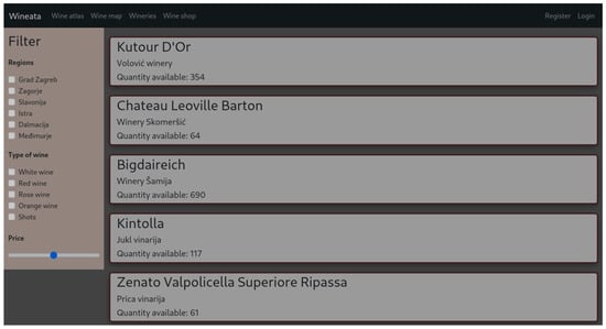
Figure 1.
Web application (a webshop) used for evaluation.
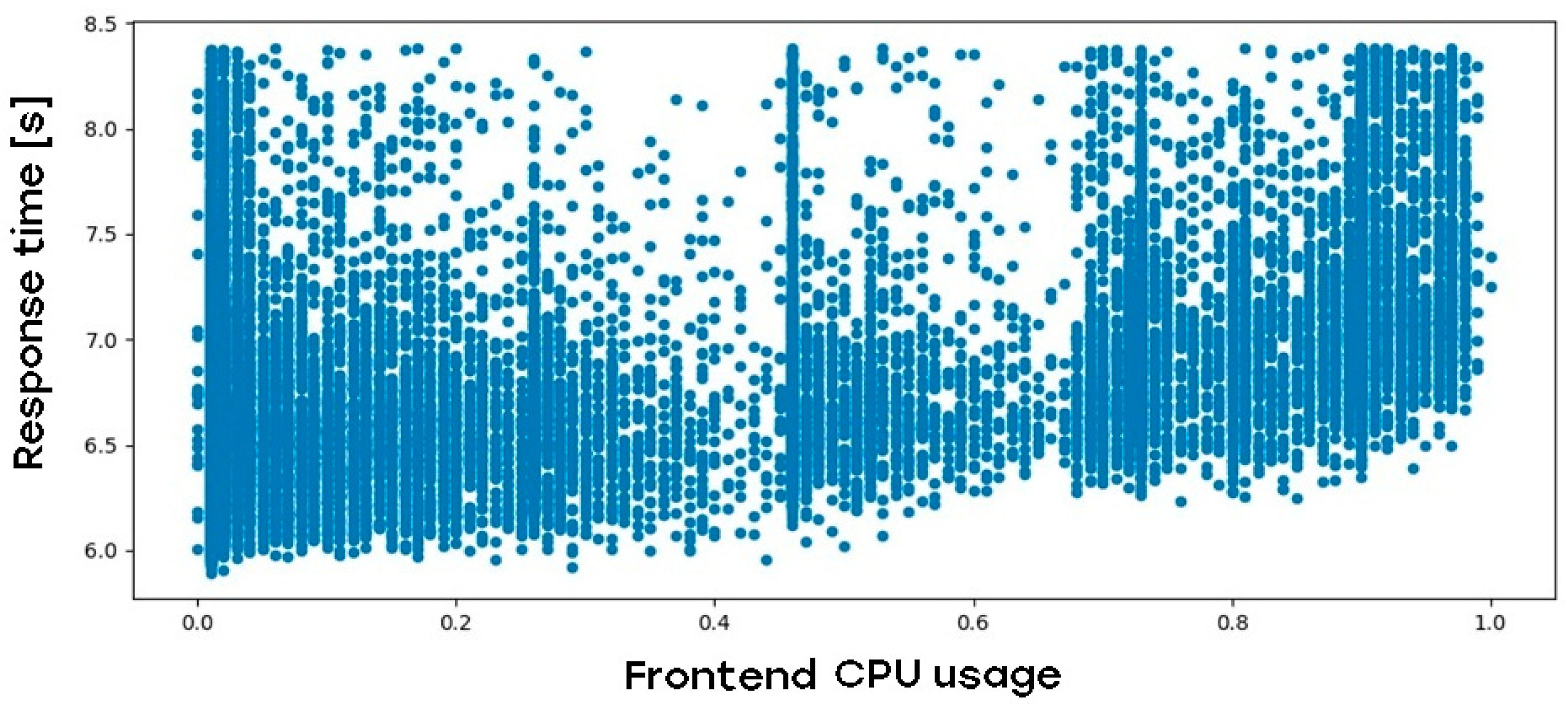
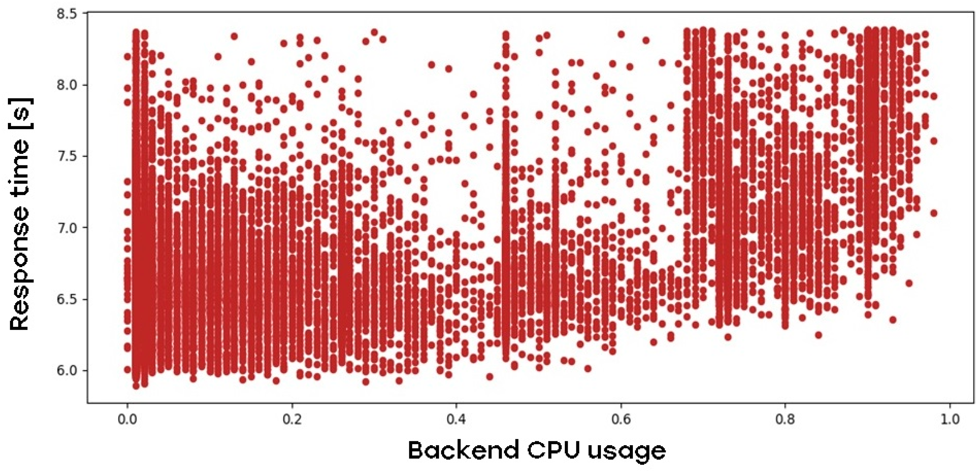
Understanding the dataset was an essential initial step in this process. Statistical analysis elucidated its structure and pinpointed potential issues that could impede the neural network’s performance. The dataset’s performance was examined under different load conditions, uncovering trends in response times. The average response time was 6.73 s, which escalated with increasing CPU load on the frontend, backend, and database nodes. The backend node demonstrated the most significant effect. Moreover, the utilization of SSDs demonstrated marginally quicker application response times relative to HDDs; however, the practical distinction was minimal. These findings emphasized the significance of hardware configuration in system performance. The average response time can be seen in Figure 2:
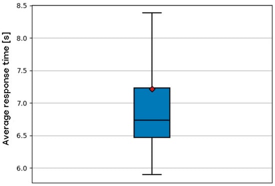
Figure 2.
Web application response time by using the default Kubernetes scheduler.
The data preparation process encompassed several essential steps to guarantee the dataset’s readiness for neural network training. The dataset in a CSV file was first imported into a Pandas DataFrame. A comprehensive cleaning procedure was conducted, encompassing identifying errors, including absent values and outliers, and their subsequent correction. The .dropna() method eliminated records with missing values, whereas outliers were discarded based on interquartile range computations. Subsequently, variables were normalized utilizing MinMaxScaler to establish consistent scales across features. This step was crucial as features with elevated numerical values could disproportionately affect the neural network. The variable frontend_pods, with a maximum value of 18, would exert a significantly more significant influence than frontend_cpu_usage, which has a maximum value of 1. Furthermore, categorical variables were converted into numerical formats through one-hot encoding to guarantee compatibility with the neural network. The dataset was subsequently divided into training and testing subsets utilizing the train_test_split() method, establishing a basis for model training and assessment.
Figure 3 describes the relationship between the frontend CPU usage and web application response time:

Figure 3.
Impact of web application frontend-tier CPU load on web application response time.
The backend of the application also has a direct influence on the web application response time, as is shown in Figure 4:
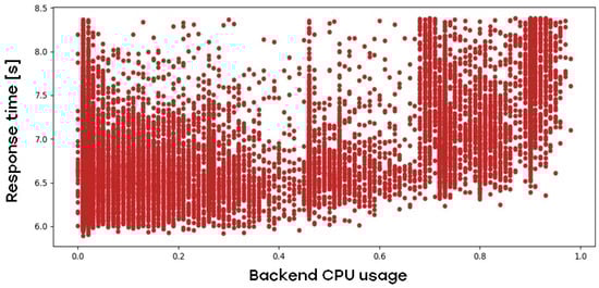
Figure 4.
Impact of web application backend-tier CPU load on web application response time.
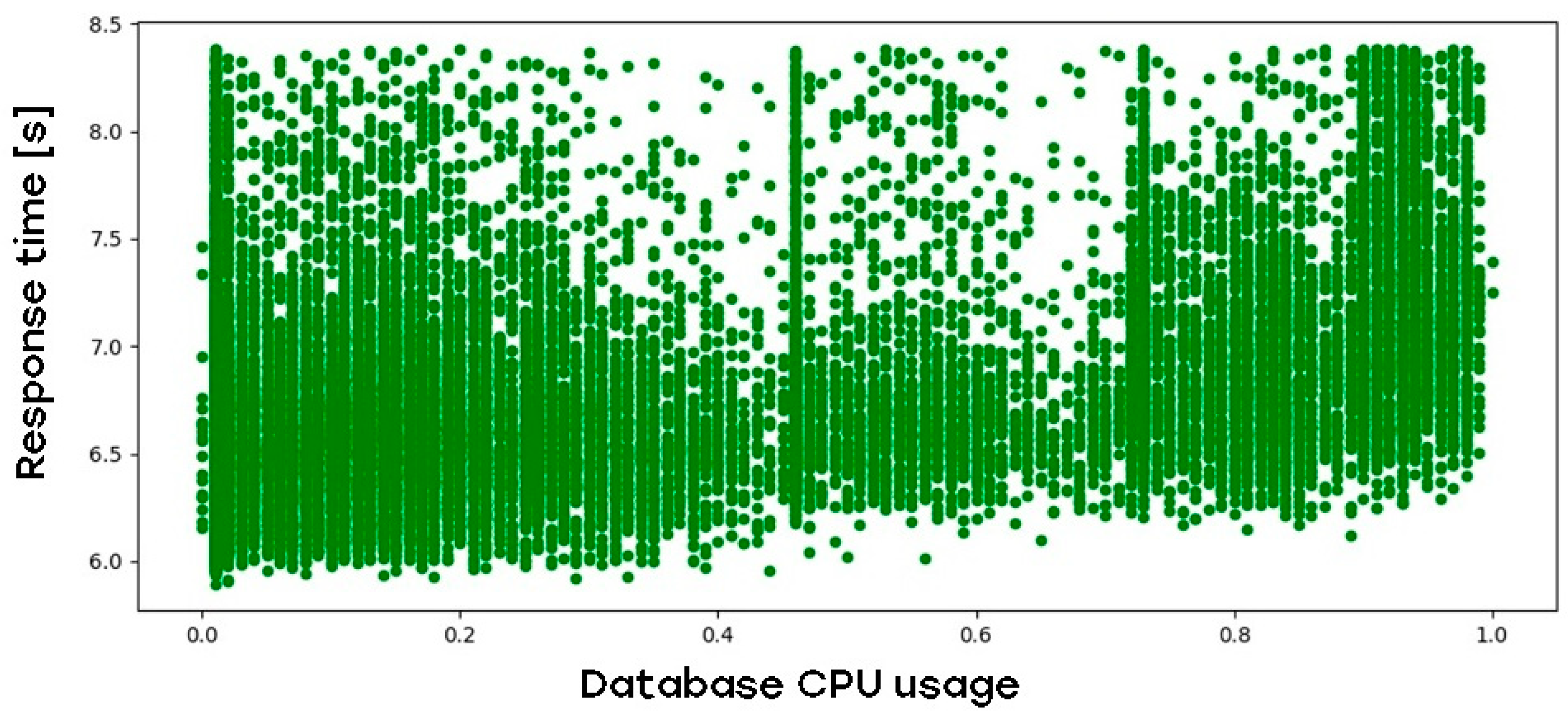
The architecture of this web application is based on the three-tier model, which means there is a separate database tier to consider. Figure 5 describes the impact of database CPU load on web application response time:

Figure 5.
Impact of web application DB tier CPU load on web application response time.
As described in Section 4, nodes with and without SSD were also considered. Figure 6 illustrates the impact of SSD on the web application response time:
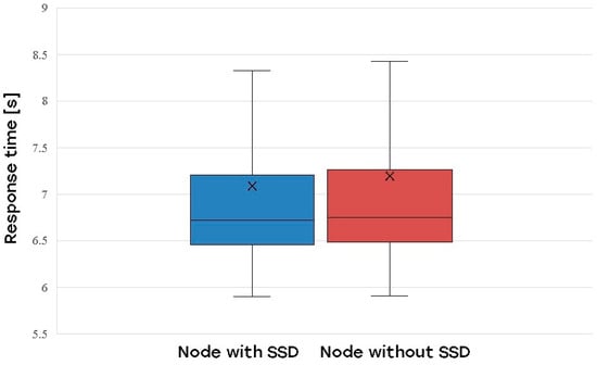
Figure 6.
Impact of SSD on web application response time.
Hyperparameter selection was guided by established best practices in machine learning literature. The initial configuration comprised 27 input neurons, one hidden layer containing ten neurons, and a single output neuron. The loss function utilized was mean squared error (MSE), and the Adam optimization algorithm was applied with a learning rate of 0.001. In the initial iteration, activation functions were not utilized in the hidden or output layers.
Enhancing the model required testing different hyperparameter configurations to augment its performance. The KerasTuner library in Python methodically identified the optimal value combinations. This tool enabled the specification of various hyperparameters, including the number of hidden layers, neurons per layer, activation functions, loss functions, and learning rates. Upon evaluating 1000 configurations, the optimal arrangement comprised four hidden layers, each containing 80 neurons, utilizing ReLU activation functions for both the hidden and output layers. The learning rate for the Adam optimizer was modified to approximately 0.00038, resulting in substantial enhancements in MSE. Hyperparameters of the neural network are shown in Table 6:
Table 6.
Neural network hyperparameters.
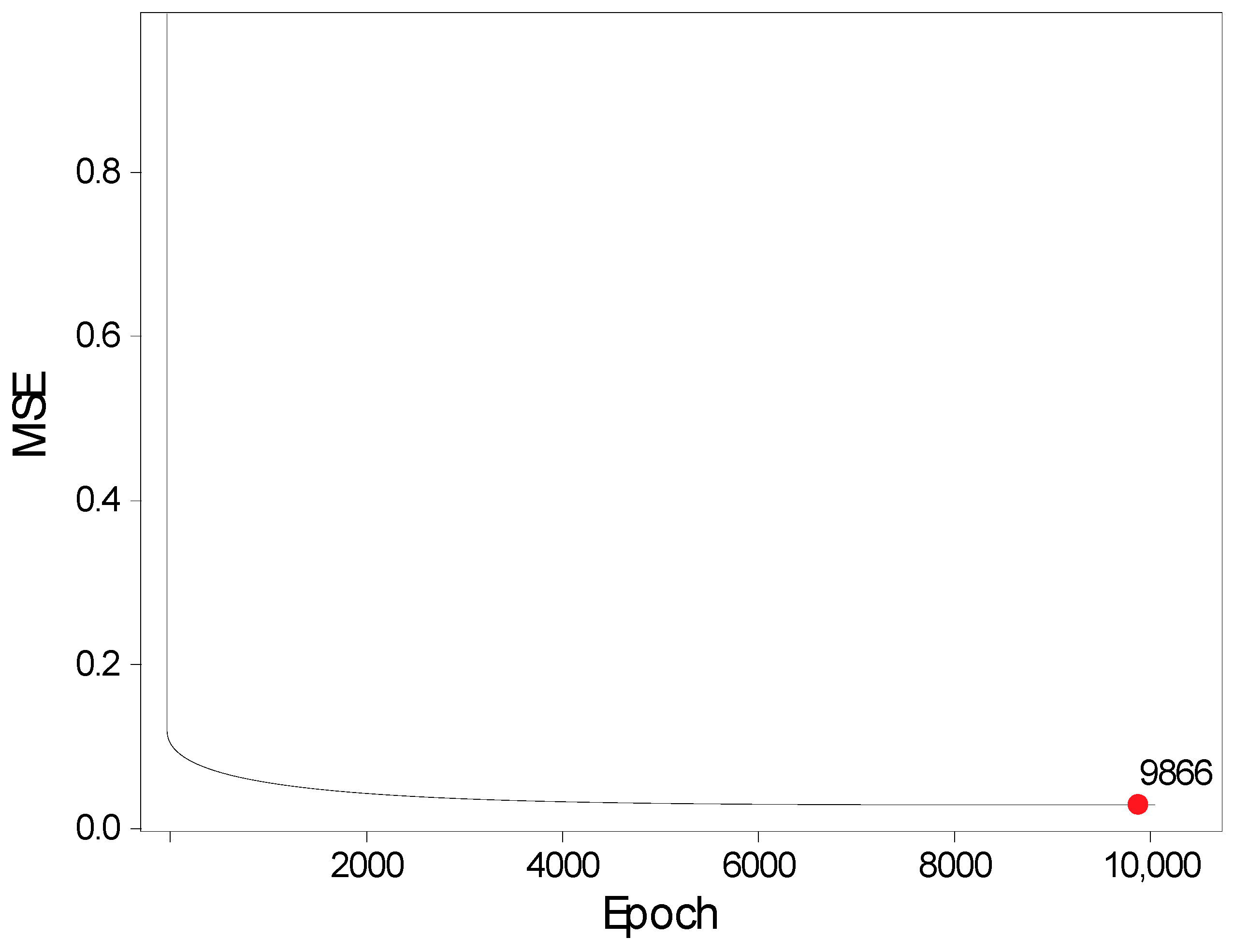
After finding the optimal values of the hyperparameters, the next step was to find the optimal number of epochs. This was performed by starting the learning process with 10,000 epochs and then looking for the epoch that contains the least MSE. It can be seen that MSE has already experienced a steep decline in the first few epochs, and after 1000 of them, the values are already less than 0.1. The lowest MSE recorded is 0.0266 at the 9866th epoch, as can be seen in Figure 7:
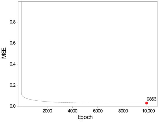
Figure 7.
MSE versus training epoch.
Although the network is still learning after 10,000 epochs, these advances are still so small that training the model in time is no longer profitable. The model was trained for 10,000 iterations to ascertain the optimal number of epochs. The mean squared error (MSE) declined significantly during the initial epochs and stabilized after roughly 1000 iterations. The minimum MSE value of 0.0266 was observed at the 9866th epoch. Nonetheless, considering the diminishing returns associated with extended training duration, the final model was trained for 5000 epochs.
The concluding phase involved testing and validating the model’s efficiency. Metrics, including mean squared error (MSE) and mean absolute error (MAE), were computed utilizing TensorFlow functions to evaluate the predictions on the test dataset. Two models were evaluated: the preliminary model, designated as Model 1, and the refined model (based on optimum hyperparameters), Model 2. Model 2 exhibited enhanced performance, attaining an MAE of 0.2975 and an MSE of 0.1431, in contrast to Model 1’s MAE of 0.3165 and MSE of 0.2039. The results, outlined in Table 7, confirmed the efficacy of the optimization process:
Table 7.
Neural network error measure metrics.
This process illustrates the iterative characteristics of machine learning model development. The analysis and preprocessing of the dataset, along with hyperparameter optimization and validation, collectively facilitated the development of a robust and efficient neural network specifically designed for the custom Kubernetes scheduler’s needs.
5. Custom Kubernetes Scheduler with Machine Learning Component
This section details the creation of a bespoke Kubernetes scheduler enhanced by a machine learning element to address the deficiencies of the standard scheduler. The custom scheduler utilizes a neural network trained on cluster resource data to resolve these difficulties. The implementation in Python commences with loading cluster setups and retrieving a list of nodes capable of executing workloads. The scheduler observes unassigned pods within the cluster’s namespace, pinpointing distinct application components, including frontend, backend, and database workloads. Upon identification, the custom scheduler assesses these workloads via the machine learning model, which forecasts response times for all potential node combinations. The model standardizes resource indicators such as CPU, RAM, and storage to guarantee precise forecasts.
5.1. How the Proposed ML Scheduler Works
The scheduler identifies optimal node combinations by selecting those within 10% of the best-expected response time. These combinations are subsequently enhanced through a grading system that evaluates storage type and resource utilization. The machine learning model facilitates equitable resource allocation, averting the overutilization of nodes or combinations. The code, constructed modularly for ease and reusability, is intended to manage dynamic workloads efficiently while markedly enhancing resource usage and application performance.
The machine learning scheduler predicts the time (in seconds) for a web application to respond. The scheduler awaits the creation of all three web application pods. Upon gathering these three components, it begins to search for a combination of nodes that will yield the most cost-effective solution. Initially, it generates estimates for all potential combinations of nodes based on resource utilization. After generating all feasible predictions, a second list containing all combinations within 10% of the best response time is created. Subsequently, it evaluates based on the following:
- Reduced resource consumption on a node;
- Storage classification: Binding pods to nodes upon identifying the most cost-effective combination.
Table 8 shows the results obtained by using the ML scheduler, compared to the default scheduler, while also measuring the predicted time and MAE:
Table 8.
Comparing default scheduler to ML scheduler.
The results indicate that the custom scheduler consistently outperforms the default scheduler in terms of time efficiency, by a margin of 1–18%, depending on the scenario. The disparity, as anticipated, between the two schedulers amplifies with the resource utilization in the cluster, with a more pronounced difference observed when three and four nodes are under load. We conclude that the disparity would be even more pronounced if the nodes within the cluster possessed not only varying resource allocations but also processors of diverse models and architectures. The mean absolute error initially diminishes with resource utilization but experiences a sharp increase when all four nodes are under load. The comprehensive implementation specifics and code are available in the source material for additional reference [29].
5.2. Results Interpretation
There are multiple reasons why the ML-based scheduler performs better than the default one. As discussed, the default scheduler has been created with the most generalized use case in mind—a deployment of a set of apps, used by Google, when developing the default scheduler. This means that it is too static to take advantage of the dynamics of a real-life, working environment, which is where ML-based schedulers, if designed properly, will be more efficient for workload scheduling.
Secondly, the default Kubernetes scheduler does not understand what a frontend or a backend of a web app is, especially in the most typical use cases, where additional parameters (CPU requests, limits etc.) are not used. The proposed ML-based scheduler is specifically trained with a tiered approach in mind, giving it more chance for more optimized workload placement.
The default scheduler also doesn’t explicitly consider CPU speed or core count—it just checks if a node has enough allocatable resources to fit a Pod. In larger environments, this commonly leads to a situation where workloads are unbalanced across the nodes. Also worth noting is the fact that the ML-based scheduler can be re-trained if the environment changes, or trained in any new environment, therefore customizing the scheduler behavior to suit that specific environment.
6. Future Works
The research detailed in this paper has multiple directions for future research that could significantly enhance the work presented in the document by addressing both the limitations of the current implementation and expanding its applicability. Initially, dynamic adaptation to resource heterogeneity would allow the scheduler to more effectively manage clusters with varied hardware architectures, including ARM and x86 processors, GPUs, and CPUs. This will enable efficient resource allocation customized to each node’s strengths, enhancing overall performance and scalability in mixed-environment installations.
Predictive maintenance enhances scheduling by utilizing system telemetry data to anticipate hardware breakdowns, as our research in another paper [30] shows. This feature could improve dependability and reduce downtime in mission-critical systems by proactively redistributing workloads to address potential concerns.
Implementing advanced learning models for scheduling optimization, such as transformers or reinforcement learning, would enhance forecast accuracy and decision-making. These sophisticated algorithms may analyze more intricate relationships within the data, resulting in more intelligent scheduling techniques that adjust to real-time dynamic workloads.
Integrating cost-conscious scheduling would synchronize resource management with economic and environmental factors. By incorporating energy efficiency and cloud pricing models, the scheduler could diminish operational costs and ecological effects, rendering it a more feasible alternative for enterprise-scale cloud installations.
Security-aware scheduling implements a crucial protective measure by favoring nodes with superior security compliance and segregating sensitive workloads. This method is especially pertinent in multi-tenant settings where data security is critical.
Finally, establishing data-driven feedback loops will perpetually enhance the scheduler’s machine learning model using real-time telemetry, guaranteeing its effective adaptation to changing workload patterns and infrastructure modifications. This adaptive learning ability would significantly improve the scheduler’s long-term efficacy and resilience.
These research directions could collectively enhance the scheduler into a more adaptable, efficient, and dependable system capable of addressing the requirements of contemporary, heterogeneous, and security-focused computing environments.
7. Conclusions
The research presented in this article demonstrates the efficiency of incorporating machine learning into Kubernetes scheduling to enhance three-tier web application load times. The custom machine learning scheduler developed in this study exhibited substantial enhancements in web application response times, particularly under conditions of heavy resource demand, surpassing the default Kubernetes scheduler. The approach utilized a neural network model trained on data from a simulated environment of a five-node Kubernetes cluster comprising one control node and four worker nodes. The three-tier application utilized in testing comprised frontend, backend, and database components, enabling the scheduler to forecast and assign the most effective node combinations for each tier based on resource utilization and response time estimations.
Artificial intelligence represents a significant milestone in contemporary society and possesses vast potential for the future. It has already achieved substantial progress across multiple domains, including healthcare, finance, transportation, and entertainment. The capacity of AI to analyze extensive datasets, identify patterns, and generate predictions has resulted in transformative progress in research, productivity, and decision-making. The creation of tools like AutoKeras, which provide user-friendly applications without necessitating prior familiarity with terminology or programming, will most benefit users who engage with technology solely for the resolution of their daily tasks.
This paper’s methodology required a way to generate a deployment, subsequently gathering all pertinent information regarding the cluster and the web application’s response time and conducting extensive manipulation of the raw data to produce a clean and usable dataset. In developing a neural network model, our primary challenge was that the literature examples either addressed the same problem using the same dataset, presented multiple methods for data preparation and model construction for regression tasks, or lacked comprehensive examples that elucidated the problem from inception through to resolution.
The architecture employed a Python-based custom scheduler that interfaced with Kubernetes APIs, utilizing TensorFlow and Keras to construct and deploy the machine learning model. Notwithstanding these gains, the implementation nonetheless entailed inevitable trade-offs. Utilizing an ML-powered scheduler necessitates supplementary computational resources, including a dedicated ML engine node, elevating infrastructure costs. Moreover, sustaining and expanding this infrastructure requires proficiency in AI and Kubernetes, posing certain obstacles for smaller or less qualified teams. There are other downsides, such as the following:
- increased infrastructure complexity;
- storing large volumes of historical data to train the ML engine to make predictions more accurate;
- a possibility of bias if data are incomplete or outdated;
- unless reinforced learning is applied, there is a risk of a model drift;
- there is a potential for unintended bias; for example, if the ML model learns from past inefficiencies or specific environmental quirks, it might make wrong scheduling decisions.
Despite these issues, the ML scheduler’s substantial performance enhancements and adaptability make it an attractive solution for resource-intensive, heterogeneous, and dynamic systems that require accurate and flexible task control. Future research can improve the scheduler by refining resource heterogeneity adaption, predictive maintenance, and sophisticated learning models for optimization, hence facilitating enhanced performance and scalability. Incorporating cost-effective and security-focused scheduling will enhance resource management and ensure compliance in multi-tenant systems. Finally, real-time data-driven feedback mechanisms will perpetually enhance the scheduler, rendering it more adaptable, efficient, and resilient for contemporary computing requirements.
Author Contributions
Conceptualization, V.D. and J.S.; methodology, V.D. and J.S.; software, G.Đ.; validation, V.D. and J.R.; formal analysis, G.Đ.; investigation, J.R.; resources, J.R.; data curation, J.S. and J.R.; writing—original draft preparation, V.D. and G.Đ.; writing—review and editing, V.D. and G.Đ.; visualization, J.S.; supervision, V.D. All authors have read and agreed to the published version of the manuscript.
Funding
This research received no external funding.
Data Availability Statement
The original contributions presented in this study are included in the article. Further inquiries can be directed to the corresponding author(s).
Conflicts of Interest
The authors declare no conflicts of interest.
References
- Lai, W.-K.; Wang, Y.-C.; Wei, S.-C. Delay-Aware Container Scheduling in Kubernetes. IEEE Internet Things J. 2023, 10, 11813–11824. [Google Scholar] [CrossRef]
- Mondal, S.K.; Zheng, Z.; Cheng, Y. On the Optimization of Kubernetes toward the Enhancement of Cloud Computing. Mathematics 2024, 12, 2476. [Google Scholar] [CrossRef]
- Dheeraj Konidena, S. Efficient Resource Allocation in Kubernetes Using Machine Learning. Int. J. Innov. Sci. Res. Technol. (IJISRT) 2024, 9, 557–563. [Google Scholar] [CrossRef]
- Cheng, X.; Fu, E.; Ling, C.; Lv, L. Research on Kubernetes Scheduler Optimization Based on Real Load. In Proceedings of the 2023 3rd International Conference on Electronic Information Engineering and Computer Science (EIECS), Changchun, China, 22–24 September 2023; pp. 711–716. [Google Scholar] [CrossRef]
- Nguyen, N.; Kim, T. Toward Highly Scalable Load Balancing in Kubernetes Clusters. IEEE Commun. Mag. 2020, 58, 78–83. [Google Scholar] [CrossRef]
- Jiao, Q.; Xu, B.; Fan, Y. Design of Cloud Native Application Architecture Based on Kubernetes. In Proceedings of the 2021 IEEE Intl Conf on Dependable, Autonomic and Secure Computing, Intl Conf on Pervasive Intelligence and Computing, Intl Conf on Cloud and Big Data Computing, Intl Conf on Cyber Science and Technology Congress (DASC/PiCom/CBDCom/CyberSciTech), Online, AB, Canada, 25–28 October 2021; pp. 494–499. [Google Scholar] [CrossRef]
- Dakić, V.; Kovač, M.; Slovinac, J. Evolving High-Performance Computing Data Centers with Kubernetes, Performance Analysis, and Dynamic Workload Placement Based on Machine Learning Scheduling. Electronics 2024, 13, 2651. [Google Scholar] [CrossRef]
- Dakić, V.; Redžepagić, J.; Bašić, M.; Žgrablić, L. Methodology for Automating and Orchestrating Performance Evaluation of Kubernetes Container Network Interfaces. Computers 2024, 13, 283. [Google Scholar] [CrossRef]
- Dakić, V.; Redžepagić, J.; Bašić, M.; Žgrablić, L. Performance and Latency Efficiency Evaluation of Kubernetes Container Network Interfaces for Built-In and Custom Tuned Profiles. Electronics 2024, 13, 3972. [Google Scholar] [CrossRef]
- Misale, C.; Drocco, M.; Milroy, D.J.; Gutierrez, C.E.A.; Herbein, S.; Ahn, D.H.; Park, Y. It’s a Scheduling Affair: GROMACS in the Cloud with the KubeFlux Scheduler. In Proceedings of the 2021 3rd International Workshop on Containers and New Orchestration Paradigms for Isolated Environments in HPC (CANOPIE-HPC), St. Louis, MO, USA, 14 November 2021; pp. 10–16. [Google Scholar] [CrossRef]
- Jian, Z.; Xie, X.; Fang, Y.; Jiang, Y.; Lu, Y.; Dash, A.; Li, T.; Wang, G. DRS: A Deep Reinforcement Learning Enhanced Kubernetes Scheduler for Microservice-based System. Softw. Pract. Exp. 2023, 54, 2102–2126. [Google Scholar] [CrossRef]
- Medel, V.; Tolón, C.; Arronategui, U.; Tolosana-Calasanz, R.; Bañares, J.Á.; Rana, O.F. Client-Side Scheduling Based on Application Characterization on Kubernetes. Lect. Notes Comput. Sci. 2017, 10537, 162–176. [Google Scholar] [CrossRef]
- Kaur, K.; Garg, S.; Kaddoum, G.; Ahmed, S.H.; Atiquzzaman, M. KEIDS: Kubernetes-Based Energy and Interference Driven Scheduler for Industrial IoT in Edge-Cloud Ecosystem. IEEE Internet Things J. 2020, 7, 4228–4237. [Google Scholar] [CrossRef]
- Altran, L.F.; Galante, G.; Oyamada, M.S. Label-Affinity-Scheduler: Considering Business Requirements in Container Scheduling for Multi-Cloud and Multi-Tenant Environments. In Proceedings of the 2022 XII Brazilian Symposium on Computing Systems Engineering (SBESC), Fortaleza, CE, Brazil, 21–24 November 2022; pp. 1–8. [Google Scholar] [CrossRef]
- Toka, L. Ultra-Reliable and Low-Latency Computing in the Edge with Kubernetes. J. Grid. Comput. 2021, 19, 31. [Google Scholar] [CrossRef]
- Rejiba, Z.; Chamanara, J. Custom Scheduling in Kubernetes: A Survey on Common Problems and Solution Approaches. ACM Comput. Surv. 2022, 55, 1–37. [Google Scholar] [CrossRef]
- Zheng, G.; Fu, Y.; Wu, T. Research on Docker Cluster Scheduling Based on Self-Define Kubernetes Scheduler. J. Phys. Conf. Ser. 2021, 1848, 012008. [Google Scholar] [CrossRef]
- Li, T.; Qiu, L.; Chen, F.; Chen, H.; Zhou, N. CAROKRS: Cost-Aware Resource Optimization Kubernetes Resource Scheduler. In Proceedings of the 2024 9th International Conference on Cloud Computing and Big Data Analytics (ICCCBDA), Chengdu, China, 25–27 April 2024; pp. 127–133. [Google Scholar] [CrossRef]
- Luca, V.-I.; Eraşcu, M. SAGE—A Tool for Optimal Deployments in Kubernetes Clusters. In Proceedings of the 2023 IEEE International Conference on Cloud Computing Technology and Science (CloudCom), Naples, Italy, 4–6 December 2023; pp. 10–17. [Google Scholar] [CrossRef]
- Ejaz, S.; Al-Naday, M. FORK: A Kubernetes-Compatible Federated Orchestrator of Fog-Native Applications Over Multi-Domain Edge-to-Cloud Ecosystems. In Proceedings of the 2024 27th Conference on Innovation in Clouds, Internet and Networks (ICIN), Paris, France, 11–14 March 2024; pp. 57–64. [Google Scholar] [CrossRef]
- Wang, X.; Han, Y. Research on Cloud Native Batch Scheduler Technology. In Proceedings of the Fourth International Conference on Computer Science and Communication Technology (ICCSCT 2023), Wuhan, China, 11 October 2023; p. 72. [Google Scholar] [CrossRef]
- Ning, A. A Customized Kubernetes Scheduling Algorithm to Improve Resource Utilization of Nodes. In Proceedings of the 2023 3rd Asia-Pacific Conference on Communications Technology and Computer Science (ACCTCS), Shenyang, China, 25–27 February 2023; pp. 588–591. [Google Scholar] [CrossRef]
- Rahali, M.; Phan, C.-T.; Rubino, G. KRS: Kubernetes Resource Scheduler for Resilient NFV Networks. In Proceedings of the 2021 IEEE Global Communications Conference (GLOBECOM), Madrid, Spain, 7–11 December 2021; pp. 1–6. [Google Scholar] [CrossRef]
- Han, Y.; Shen, S.; Wang, X.; Wang, S.; Leung, V.C.M. Tailored Learning-Based Scheduling for Kubernetes-Oriented Edge-Cloud System. In Proceedings of the IEEE INFOCOM 2021—IEEE Conference on Computer Communications, Vancouver, BC, Canada, 10–13 May 2021. [Google Scholar] [CrossRef]
- Haja, D.; Szalay, M.; Sonkoly, B.; Pongracz, G.; Toka, L. Sharpening Kubernetes for the Edge. In Proceedings of the ACM SIGCOMM 2019 Conference Posters and Demos 2019; ACM Digital Library: New York, NY, USA, 2019. [Google Scholar] [CrossRef]
- Rothman, J.; Chamanara, J. An RL-Based Model for Optimized Kubernetes Scheduling. In Proceedings of the 2023 IEEE 31st International Conference on Network Protocols (ICNP), Reykjavik, Iceland, 10–13 October 2023; pp. 1–6. [Google Scholar] [CrossRef]
- Sun, Y.; Xiang, H.; Ye, Q.; Yang, J.; Xian, M.; Wang, H. A Review of Kubernetes Scheduling and Load Balancing Methods. In Proceedings of the 2023 4th International Conference on Information Science, Parallel and Distributed Systems (ISPDS), Guangzhou, China, 14–16 July 2023; pp. 284–290. [Google Scholar] [CrossRef]
- Dataset Generator. Available online: https://github.com/jura43/dataset-generator (accessed on 5 December 2024).
- Scheduler ML. Available online: https://github.com/jura43/ml-scheduler (accessed on 14 December 2024).
- Dakić, V.; Bertina, K.; Redžepagić, J.; Regvart, D. The RedFish API and vSphere Hypervisor API: A Unified Framework for Policy-Based Server Monitoring. Electronics 2024, 13, 4624. [Google Scholar] [CrossRef]


Disclaimer/Publisher’s Note: The statements, opinions and data contained in all publications are solely those of the individual author(s) and contributor(s) and not of MDPI and/or the editor(s). MDPI and/or the editor(s) disclaim responsibility for any injury to people or property resulting from any ideas, methods, instructions or products referred to in the content. |
© 2025 by the authors. Licensee MDPI, Basel, Switzerland. This article is an open access article distributed under the terms and conditions of the Creative Commons Attribution (CC BY) license (https://creativecommons.org/licenses/by/4.0/).