An Approach to Control Multilevel Flying-Capacitor Converters Using Optimal Dynamic Programming Benchmark

Abstract

The problem of balancing capacitor voltages is of utmost importance in multilevel converter topologies involving flying capacitors. In this study, a new minimum angular distance (MAD) algorithm is proposed to control the turning on and off of the switches, ensuring fast convergence of the capacitor voltages balancing problem in multilevel flying-capacitor converters. This algorithm was developed based on a preliminary analytical analysis of the capacitor voltage trajectories using the power-oriented model of the converter. Compared to other approaches, the proposed algorithm involves only simple and well-defined calculations, requires no training, and does not require any prediction of future values that the output current assumes. The proposed algorithm, implemented in the MATLAB/Simulink environment, is proven to give very good performance, verified against an optimal benchmark given by dynamic programming, in terms of capacitor voltages convergence time, efficiency, power loss, and total harmonic distortion.

1. Introduction

Electrical power conversions find several applications, including power grids [1], the control [2] of electric machines [3], electric vehicles [4], and many others. Power converters can be mainly classified into DC/DC [4,5,6], AC/DC [7], DC/AC [8], and AC/AC converters [9,10,11]. Strong research interest resides in multilevel converters thanks to the many advantages they offer over two-level converters  [12,13]. The multilevel converter topologies available in the literature include modular converters [14], H-bridge converters [15], and flying-capacitor converters [8].

In order to study the considered converter topology, the modeling step is the first to be addressed, as shown in [16] for switched systems. The modeling of cascaded H-bridge multilevel inverters is addressed in [15] using Kirchhoff’s laws, whereas the modeling of modular multilevel converters is addressed in [17] using a state-space approach. In [18], the authors address the modeling of the considered DC microgrid by providing the differential equations describing it, whereas an effective approach for modeling multilevel flying-capacitor converters is proposed in [8] using the Power-Oriented Graphs modeling technique [19,20]. The next important step to be addressed is converter control [21], both for DC/DC and for AC/DC–DC/AC converters. The optimal control of buck converters is addressed in [22] with the objective of keeping the output voltage as close to the desired setpoint as possible. Weighted model predictive control is applied to modular multilevel converters in [23], whereas an approach for controlling multilevel flying-capacitor converters with varying numbers of output voltage levels is proposed in [8]. When working with converter topologies involving floating capacitors, a particularly delicate aspect is the capacitor voltages balancing issue [24,25] in order to have a proper output voltage waveform. Different approaches are available in the literature to guarantee the balancing of capacitor voltages, which can vary from different modulation techniques [25,26,27] to the use of closed-loop techniques [28,29,30,31]. A new pulse width modulation (PWM) method was proposed in [25], while Phase Disposition PWM (PDPWM) is proposed in [26]. A modified version of Carrier-Redistribution PWM (CRPWM) was employed in [27] instead, allowing low voltage ripple and low harmonic content in the output voltage. On the other hand, closed-loop methods have the advantage of being more robust against undesired situations such as faults [8], for example. A closed-loop approach for capacitor voltages balancing is proposed in [28], introducing a dedicated control signal that modifies the duty cycle generated through modulation, while a deadband-based method is proposed in [29]. Other available closed-loop approaches can foresee the use of a proportional-integral controller [30] to achieve capacitor voltage balancing or a cost function to be minimized [31]. A common closed-loop approach for controlling power converters is model predictive control (MPC) [32]. As an example, in [33] the authors use an MPC variant to minimize a cost function using several criteria, including output voltage tracking and capacitor voltages balancing. However, this approach requires the prediction of the future values that the output current assumes. Furthermore, whenever a cost function needs to be minimized, the choice of weighting factors comes into play, which is generally not trivial. MPC is also used in [34] to minimize a cost function, involving output current tracking and capacitor voltages. Even in this case, however, output current prediction is required, and the weighting factors tuning problem was addressed by finding the proper weighting factors experimentally to minimize the total harmonic distortion. A switching control law is proposed in [35] instead, in order to achieve output voltage control and flying-capacitor voltages balancing in a four-level flying-capacitor converter. In [36], an artificial neural network was used to control a multilevel flying-capacitor inverter instead. The neural network was trained using data from the inverter controlled by MPC to achieve capacitor voltages balancing and output current tracking. However, the neural network training process is no easy task, as the input features need to be chosen. The use of neural networks is indeed becoming popular in several engineering applications, including power electronics [37] for applications such as capacitor voltages estimation [38] and converter control [36,39]. As an example, an artificial neural network is employed in [38] for capacitor voltages estimation, and a deep neural network is used in [39] to control multilevel flying-capacitor converters after a training phase from converter operations controlled using MPC. However, the difficulty in these approaches is represented by the training phase, where the right number of samples must be chosen in order to avoid, for example, underfitting or overfitting problems.

In the present paper, multilevel flying-capacitor converters (MFCCs) are the subject of study. A new control algorithm is proposed, handling the turning on and off of the switches to ensure fast convergence regarding the capacitor voltages balancing problem. The proposed control algorithm has the beneficial properties of being effective and simple to implement, as it is based on the calculation of the angular distance between vectors. Specifically, the work in [8] is extended with the following contributions with respect to the literature:

(1) A detailed analysis of the converter dynamics, with specific emphasis on the IGBT (Insulated Gate Bipolar Transistor) signals’ impact on the evolution of the capacitor voltage trajectories, with the objective of proposing the new algorithm at the next point; (2) a new minimum angular distance (MAD) control algorithm is proposed. The algorithm handles the turning on and off of the switches to ensure the fast balancing of capacitor voltages in multilevel flying-capacitor converters with a generic number n of capacitors. The proposed MAD algorithm exhibits the following features: it involves very simple and well-defined calculations and does not require any training or prediction regarding future values that the output current assumes. The proposed algorithm is causal and implementable in real time. Furthermore, it can be applied to multilevel flying capacitor converters with a generic number n of capacitors, and it is proven to exhibit convergence times and performance in terms of efficiency, power loss, and total harmonic distortion (THD) which are very close to those provided by the considered optimal benchmark; (3) the statement and the description of the optimal control problem aiming at achieving balanced capacitor voltages condition. The optimal control sequence of the IGBTs states allowing the obtainment of such conditions, while generating the desired output voltage, is found using dynamic programming (DP) [40,41]. The latter approach requires a priori knowledge of the converter cycle, which makes it noncausal and not implementable in real time. However, DP represents an optimal benchmark candidate for evaluating the performance of the proposed MAD algorithm. Dynamic programming is used to generate the optimal benchmark because it is a well-established method to achieve the optimal solution given by Bellman’s Principle of Optimality [40]; (4) the evaluation of the good performance of the MAD algorithm by comparing the obtained results with those given by the DP optimal benchmark in terms of capacitors voltages convergence time, efficiency, power loss, and output voltage total harmonic distortion (THD).

The remainder of this paper is organized as follows. The converter modeling, voltage trajectories dynamic analysis, and converter control using the MAD algorithm are addressed in Section 2, Section 3, and Section 3.1, respectively. The optimal control problem is stated in Section 3.2, whereas a comparison of the results between the MAD algorithm and DP is addressed in Section 4. Finally, the conclusions are reported in Section 5.

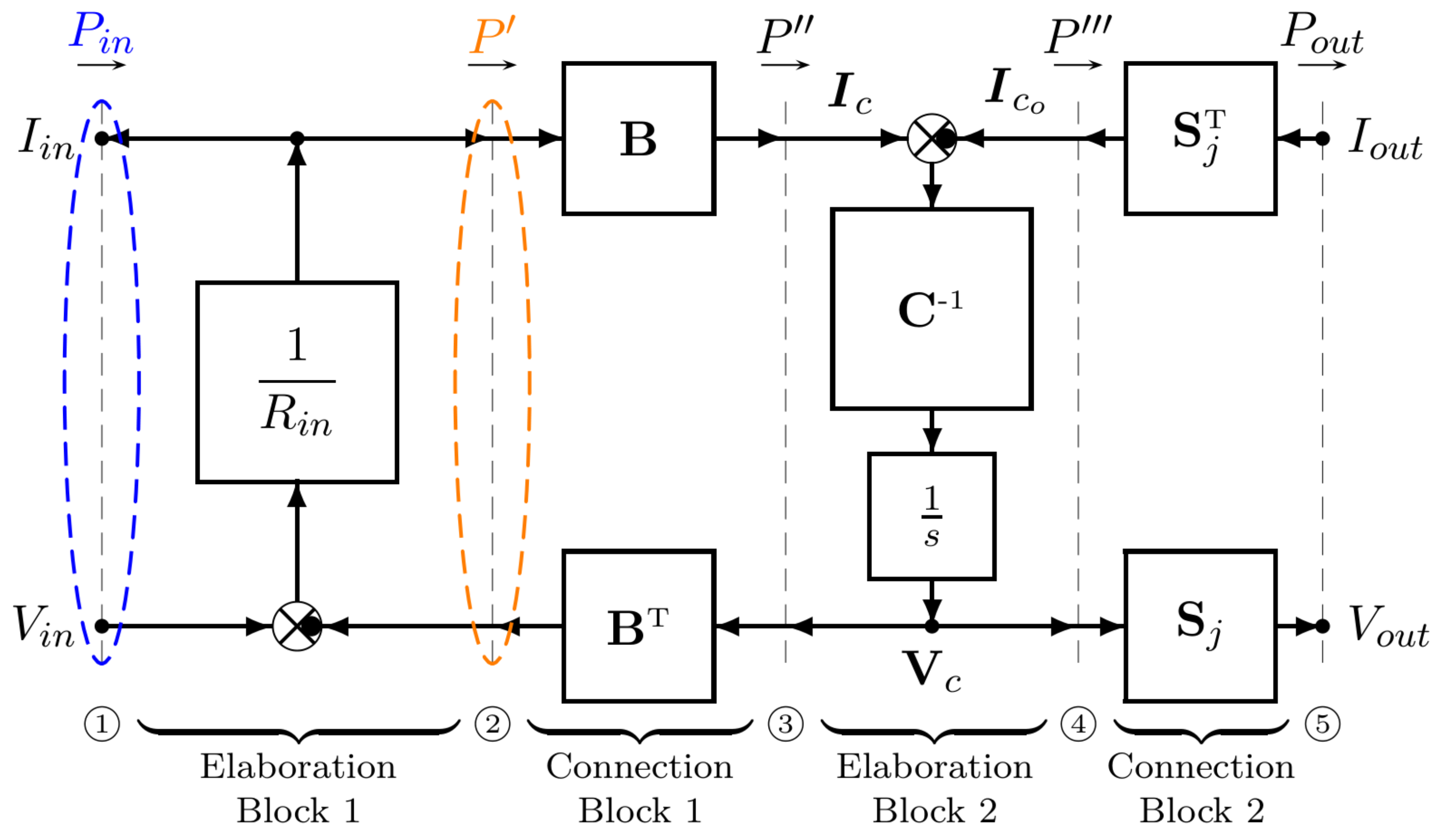
2. Converter Modeling

The circuital representation of the n-dimensional multilevel flying-capacitor converter used for the proposed analysis is shown in Figure 1. This converter can be modeled as [8]:

$$\begin{gathered} \left\{\begin{array}{c}\mathbf{C}{\dot{\mathbf{V}}}_c=\mathbf{A}{\mathbf{V}}_c+\left[\begin{array}{cc}\mathbf{B}& -{\mathbf{S}}_j^T\end{array}\right]\mathit{u},\\ \mathbf{y}=\left[\begin{array}{c}-{\mathbf{B}}^T\\ {\mathbf{S}}_j\end{array}\right]{\mathbf{V}}_c+\mathbf{D}\mathit{u},\end{array}\right.\mathbf{C}=\left[\begin{array}{cccc}{C}_1& 0& \cdots & 0\\ 0& C_2& \cdots & 0\\ ⋮& ⋮& \ddots & ⋮\\ 0& 0& \cdots & C_n\end{array}\right], \\ \mathbf{A}=\left[\begin{array}{cccc}{\displaystyle \frac{-1}{R_{in}}}& 0& \cdots & 0\\ 0& 0& \cdots & 0\\ ⋮& ⋮& \ddots & ⋮\\ 0& 0& \cdots & 0\end{array}\right],{\mathbf{V}}_c=\left[\begin{array}{c}{V}_1\\ V_2\\ ⋮\\ V_n\end{array}\right],{\mathbf{S}}_j^T=\left[\begin{array}{c}{s}_1\\ s_2\\ ⋮\\ s_n\end{array}\right],\mathbf{B}=\left[\begin{array}{c}{\displaystyle \frac{1}{R_{in}}}\\ ⋮\\ 0\end{array}\right], \\ \mathbf{D}=\left[\begin{array}{cc}{\displaystyle \frac{1}{R_{in}}}& 0\\ 0& 0\end{array}\right],\mathbf{y}=\left[\begin{array}{c}{I}_{in}\\ V_{out}\end{array}\right],\mathit{u}=\left[\begin{array}{c}{V}_{in}\\ I_{out}\end{array}\right], \end{gathered}$$

(1)

where $\mathbf{C}$ and $\mathbf{A}$ are the system energy matrix and the system power matrix, respectively, ${\mathbf{V}}_c$, $\mathit{u}$, and $\mathbf{y}$ are the system state, input and output vectors, respectively, and n is the number of capacitors in the converter. Vector ${\mathbf{S}}_j\in {\mathbb{R}}^{(1\times n)}$ in (1) is called configuration vector. The state-space model (1) of the considered flying-capacitor multilevel converter can be equivalently represented using the Power-Oriented Graphs (POG) block scheme in Figure 2 [8]. The vertical dashed lines in the figure are named power sections and describe the power flows within the considered flying-capacitor multilevel converter. The first elaboration block in Figure 2 describes the input resistance, while the second elaboration block describes the capacitor dynamics. The first connection block in Figure 2 describes the interaction between the resistive and capacitive parts of the converter, while the second connection block describes the interaction of the converter with the external world, that is, with the load. The horizontal arrows located at the top of each power section describe the positive direction of the power flows exchanged from one section to the next. When used as a DC/AC converter, $P_{in}>0$, $P^{\prime }=P^{″}>0$ and $P^{‴}=P_{out}>0$ hold. Either the condition $P^{\prime }=P^{″}>P^{‴}=P_{out}$ or the condition $P^{\prime }=P^{″}<P^{‴}=P_{out}$ can be verified depending on the configuration vector ${\mathbf{S}}_j$, which will act to either recharge or discharge the capacitors $C_1,\dots ,C_n$, as is further discussed in Section 3. Figure 2 shows that the power dissipation in the considered system takes place because of the input resistance $R_{in}$. Therefore, the system’s average efficiency $\overline{E}$ and average power loss ${\overline{P}}_l$ can be defined as:

$$\overline{E}={\displaystyle \frac{{\overline{P}}^{\prime }}{{\overline{P}}_{in}}}\mathrm{a}\mathrm{n}\mathrm{d}{\overline{P}}_l={\overline{P}}_{in}-{\overline{P}}^{\prime }$$

(2)

when the converter performs a DC/AC conversion, where ${\overline{P}}_{in}=\mathrm{m}\mathrm{e}\mathrm{a}\mathrm{n}\left(P_{in}\right)$ and ${\overline{P}}^{\prime }=\mathrm{m}\mathrm{e}\mathrm{a}\mathrm{n}\left(P^{\prime }\right)$.

Vector ${\mathbf{S}}_j$ in (1) is in one-to-one correspondence with the IGBT signal vector ${\mathbf{T}}_j$ through the following property [8]:

Property 1.

The components $s_i\in \{-1,0,1\}$ of the configuration vector ${\mathbf{S}}_j=\left[s_1{s}_2\cdots s_n\right]$ can be obtained from the components $T_i\in \{0,1\}$ of the IGBT signal vector ${\mathbf{T}}_j=\left[T_1{T}_2\cdots T_n\right]$ as follows:

$$s_i=\left\{\begin{array}{ccc}{T}_1& if\hfill & i=1,\hfill \\ {\overline{T}}_{i-1}{T}_i-T_{i-1}{\overline{T}}_i& if\hfill & i\in \left\{2,\cdots ,n\right\}.\hfill \end{array}\right.$$

(3)

The index $j\in \{0,1,\dots ,2^n-1\}$ identifies all the different $2^n$ combinations that the IGBT signals can assume. The study reported in [8] indicates that a different number $m=n+1\dots 2^n$ of output voltage levels can be obtained by properly choosing the desired reference values for the capacitor voltages. In the case of $n=3$, the converter operates in the so-called basic mode, generating $m=4$ output voltage levels if the capacitors’ voltages are controlled to the following desired reference values:

$${\mathbf{V}}_{c_d}={\left[\begin{array}{ccc}{V}_{1_d}& V_{2_d}& V_{3_d}\end{array}\right]}^T={\left[\begin{array}{ccc}{V}_{in}& {\displaystyle \frac{2V_{in}}{3}}& {\displaystyle \frac{V_{in}}{3}}\end{array}\right]}^T,$$

(4)

where $V_{in}$ is the DC input voltage, as shown in Figure 1. The resulting output voltage levels are shown in

Table 1. Switching table relating the IGBT signals to the values of the output voltage $V_{out}$ when $n=3$.

${\mathbf{T}}_{\mathit{j}}$	$T_1$	$T_2$	$T_3$	$V_{out}$ (if (4) holds)	Level
${\mathbf{T}}_0$	0	0	0	0	${\mathrm{L}}_0$
${\mathbf{T}}_1$	0	0	1	$V_3={\displaystyle \frac{V_{in}}{3}}$	${\mathrm{L}}_1$
${\mathbf{T}}_2$	0	1	0	$V_2-V_3={\displaystyle \frac{V_{in}}{3}}$	${\mathrm{L}}_1$
${\mathbf{T}}_3$	0	1	1	$V_2={\displaystyle \frac{2V_{in}}{3}}$	${\mathrm{L}}_2$
${\mathbf{T}}_4$	1	0	0	$V_1-V_2={\displaystyle \frac{V_{in}}{3}}$	${\mathrm{L}}_1$
${\mathbf{T}}_5$	1	0	1	$V_1-V_2+V_3={\displaystyle \frac{2V_{in}}{3}}$	${\mathrm{L}}_2$
${\mathbf{T}}_6$	1	1	0	$V_1-V_3={\displaystyle \frac{2V_{in}}{3}}$	${\mathrm{L}}_2$
${\mathbf{T}}_7$	1	1	1	$V_1=V_{in}$	${\mathrm{L}}_3$

.

Discrete-Time Model

The set of state transition equations in (1) can be rewritten as

$${\dot{\mathbf{V}}}_c=\underset{\overline{\mathbf{A}}}{\underbrace{{\mathbf{C}}^{-1}\mathbf{A}}}{\mathbf{V}}_c+\underset{\overline{\mathbf{B}}}{\underbrace{{\mathbf{C}}^{-1}\left[\begin{array}{cc}\mathbf{B}& -{\mathbf{S}}_j^T\end{array}\right]}}\mathit{u},$$

(5)

where vectors ${\mathit{V}}_c$, $\mathit{B}$, ${\mathit{S}}_j$, $\mathit{u}$ and matrices $\mathit{A}$, $\mathit{C}$ are defined in (1).

In the case of $n=3$, matrices $\overline{\mathbf{A}}$ and $\overline{\mathbf{B}}$ in (5) assume the following form:

$$\overline{\mathbf{A}}=\left[\begin{array}{ccc}-{\displaystyle \frac{1}{C_1{R}_{in}}}& 0& 0\\ 0& 0& 0\\ 0& 0& 0\end{array}\right],\overline{\mathbf{B}}=\left[\begin{array}{cc}{\displaystyle \frac{1}{C_1{R}_{in}}}& -{\displaystyle \frac{s_1}{C_1}}\\ 0& -{\displaystyle \frac{s_2}{C_2}}\\ 0& -{\displaystyle \frac{s_3}{C_3}}\end{array}\right],$$

(6)

and Equations (5) and (6) can be discretized into the following matrix difference equation:

$$\begin{array}{c}{\mathit{V}}_c(k+1)=\mathit{F}{\mathit{V}}_c\left(k\right)+\mathit{G}\mathit{u}\left(k\right),\mathbf{F}=e^{\overline{\mathit{A}}{T}_s},\mathbf{G}={\int }_0^{T_s}{e}^{\overline{\mathbf{A}}\sigma }\overline{\mathbf{B}}d\sigma ,\hfill \\ \mathbf{F}=\left[\begin{array}{ccc}{e}^{{\displaystyle \frac{-T_s}{C_1{R}_{in}}}}& 0& 0\\ 0& 1& 0\\ 0& 0& 1\end{array}\right],\mathbf{G}=\left[\begin{array}{cc}1-e^{{\displaystyle \frac{-T_s}{C_1{R}_{in}}}}& -s_1{R}_{in}\left(1-e^{{\displaystyle \frac{-T_s}{C_1{R}_{in}}}}\right)\\ 0& {\displaystyle \frac{-T_s{s}_2}{C_2}}\\ 0& {\displaystyle \frac{-T_s{s}_3}{C_3}}\end{array}\right],\hfill \end{array}$$

(7)

where $T_s$ is the sampling time.

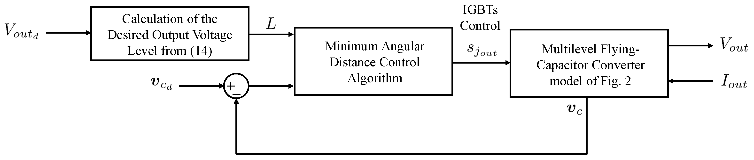
3. Converter Control

The set of state transition equations in (1) can be rewritten as [8]:

$${\dot{\mathbf{V}}}_c={\mathbf{C}}^{-1}\mathbf{A}{\mathbf{V}}_c\underset{{\tilde{\mathbf{S}}}_j^T}{\underbrace{-{\mathbf{C}}^{-1}{\mathbf{S}}_j^T}}{I}_{out}+{\mathbf{C}}^{-1}\mathbf{B}{V}_{in},$$

(8)

where ${\tilde{\mathbf{S}}}_j$ represents a new version of the configuration vector ${\mathbf{S}}_j$, in which the i-th component of ${\mathbf{S}}_j$ has been normalized with respect to the i-th capacitance $C_i$. Since the value of the input resistance $R_{in}$ is typically very low [8], from the first equation in (8) it can be evinced that $V_1\simeq V_{in}$, meaning that the number of capacitor voltages to be controlled changes from n to $n-1$. Therefore, a reduced version ${\tilde{\mathbf{s}}}_j$ of the configuration vector ${\tilde{\mathbf{S}}}_j$ can be introduced:

$${\tilde{\mathbf{s}}}_j=\left[s_2/C_2\cdots s_n/C_n\right].$$

(9)

From the reduced vector ${\tilde{\mathbf{s}}}_j$, the reduced configuration versor ${\mathbf{s}}_j$ can be defined as follows:

$${\mathbf{s}}_j={\tilde{\mathbf{s}}}_j/\parallel {\tilde{\mathbf{s}}}_j\parallel ,$$

(10)

which will be called control versor ${\mathbf{s}}_j$ hereafter. For the case of $n=3$, all the possible control versors ${\mathbf{s}}_j$ that can be obtained from all the possible IGBT signal vectors ${\mathbf{T}}_j$ in Table 1 can be found using (3), (9), and (10) as follows:

$$\left[\begin{array}{c}{\mathbf{T}}_0\\ {\mathbf{T}}_1\\ {\mathbf{T}}_2\\ {\mathbf{T}}_3\\ {\mathbf{T}}_4\\ {\mathbf{T}}_5\\ {\mathbf{T}}_6\\ {\mathbf{T}}_7\end{array}\right]=\left[\begin{array}{ccc}\hfill 0& \hfill 0& \hfill 0\\ \hfill 0& \hfill 0& \hfill 1\\ \hfill 0& \hfill 1& \hfill 0\\ \hfill 0& \hfill 1& \hfill 1\\ \hfill 1& \hfill 0& \hfill 0\\ \hfill 1& \hfill 0& \hfill 1\\ \hfill 1& \hfill 1& \hfill 0\\ \hfill 1& \hfill 1& \hfill 1\end{array}\right]\iff \left[\begin{array}{c}{\mathbf{s}}_0\\ {\mathbf{s}}_1\\ {\mathbf{s}}_2\\ {\mathbf{s}}_3\\ {\mathbf{s}}_4\\ {\mathbf{s}}_5\\ {\mathbf{s}}_6\\ {\mathbf{s}}_7\end{array}\right]=\left[\begin{array}{cc}0& 0\\ 0& 1\\ {\displaystyle \frac{1}{C_2\parallel {\tilde{s}}_2\parallel }}& -{\displaystyle \frac{1}{C_3\parallel {\tilde{s}}_2\parallel }}\\ 1& 0\\ -1& 0\\ -{\displaystyle \frac{1}{C_2\parallel {\tilde{s}}_5\parallel }}& {\displaystyle \frac{1}{C_3\parallel {\tilde{s}}_5\parallel }}\\ 0& -1\\ 0& 0\end{array}\right].$$

(11)

Remark 1.

From (8)–(10), and recalling that $V_1\simeq V_{in}$, it can be observed that

$${\dot{V}}_i=-{\mathbf{s}}_j\parallel {\tilde{\mathbf{s}}}_j\parallel I_{out},fori=2,\dots ,n,$$

(12)

meaning that the trajectory of the reduced voltage vector ${\mathit{v}}_c={\left[\begin{array}{ccc}\hfill V_2& \hfill \dots & \hfill V_n\end{array}\right]}^T$ moves in the $n-1$ dimensional state-space $(V_2,\dots ,V_n)$ in the direction specified by the control versor ${\mathbf{s}}_j$ when $I_{out}<0$, and it moves in the opposite direction when $I_{out}>0$. The distance covered by the reduced voltage vector ${\mathit{v}}_c={\left[\begin{array}{ccc}\hfill V_2& \hfill \dots & \hfill V_n\end{array}\right]}^T$ is given by $\parallel {\tilde{\mathbf{s}}}_j\parallel |I_{out}|$.

A graphical representation of the direction imposed on the trajectory of the reduced voltage vector ${\mathit{v}}_c={\left[\begin{array}{cc}\hfill V_2& \hfill V_3\end{array}\right]}^T$ by the control versors ${\mathbf{s}}_0$, ${\mathbf{s}}_1$, ${\mathbf{s}}_2$, ${\mathbf{s}}_3$, ${\mathbf{s}}_4$, ${\mathbf{s}}_5$, ${\mathbf{s}}_6$, and ${\mathbf{s}}_7$ in the state-space $(V_2,V_3)$ for $n=3$ is shown in Figure 3, assuming the following ratios between the capacitors values [8]:

$$C_1={\displaystyle \frac{C_3}{3}},C_2={\displaystyle \frac{C_3}{2}},C_3.$$

(13)

From (11), (12), Table 1, and Figure 3, it can be observed that: (1) when the levels ${\mathrm{L}}_0$ or ${\mathrm{L}}_3$ need to be generated, the trajectory of the reduced voltage vector ${\mathit{v}}_c$ does not move since the control versors ${\mathbf{s}}_0$ or ${\mathbf{s}}_7$ are null; (2) when the levels ${\mathrm{L}}_1$ or ${\mathrm{L}}_2$ need to be generated, the direction of (and the distance covered by) the trajectory of the reduced voltage vector ${\mathit{v}}_c$ depend on the control versor that is used: ${\mathbf{s}}_1$, ${\mathbf{s}}_2$, or ${\mathbf{s}}_4$ for level ${\mathrm{L}}_1$, and ${\mathbf{s}}_3$, ${\mathbf{s}}_5$, or ${\mathbf{s}}_6$ for level ${\mathrm{L}}_2$.

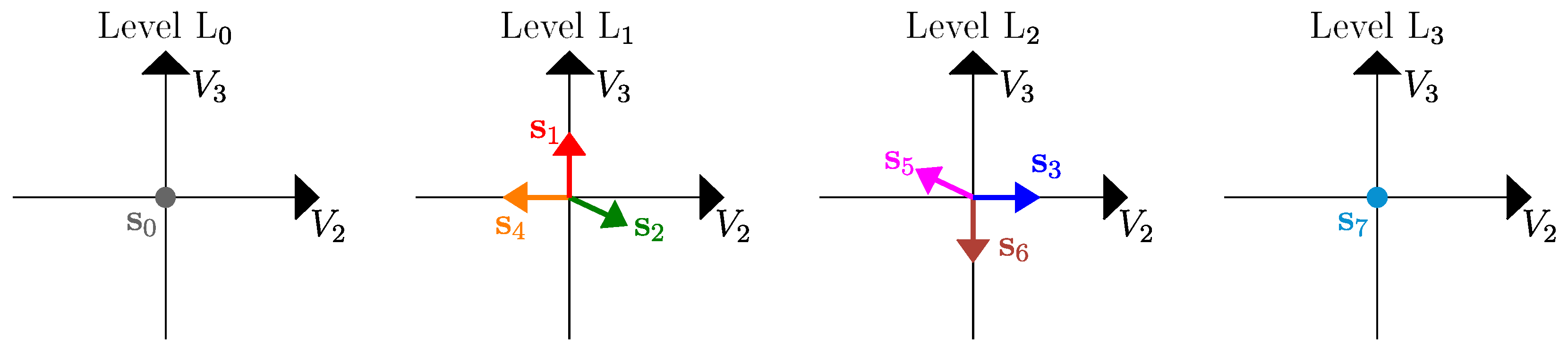
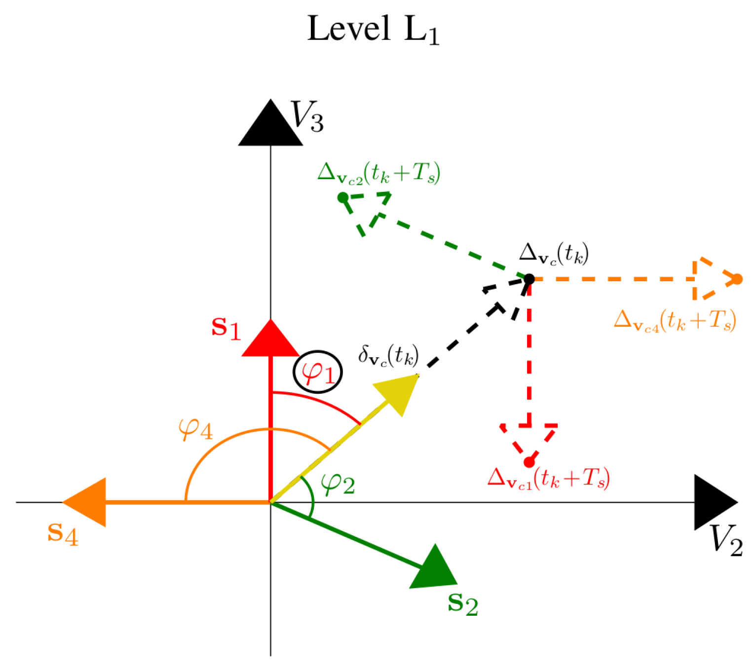
3.1. Proposed Minimum Angular Distance (MAD) Control

Let $V_{ou{t}_d}$ be the desired sinusoidal profile for the output voltage $V_{out}$ indicated in Figure 1, let $T_{PWM}$ be the pulse width modulation period, let $\delta$ be the duty cycle, and let $t_k$ be the current time instant. Let $V^{-}$ and $V^{+}$ be the two voltage values associated with the lower and upper levels ${\mathrm{L}}^{-}$ and ${\mathrm{L}}^{+}$, between which voltage $V_{ou{t}_d}$ falls within the $T_{PWM}$ period. The desired output voltage level L within each $T_{PWM}$ period is given by:

$$\mathrm{L}=\left\{\begin{array}{ccc}{\mathrm{L}}^{-}\hfill & \mathrm{for}\hfill & [t_k,t_k+\delta T_{PWM})\hfill \\ {\mathrm{L}}^{+}\hfill & \mathrm{for}\hfill & [t_k+\delta T_{PWM},t_k+T_{PWM})\hfill \end{array}\right..$$

(14)

Let ${\mathit{v}}_{c_d}={\left[\begin{array}{ccc}{V}_{2_d}& \dots & V_{n_d}\end{array}\right]}^T$ be the desired reference for the reduced voltage vector ${\mathit{v}}_c$ introduced in Remark 1, and let ${\Delta }_{{\mathit{v}}_c}={\mathit{v}}_c-{\mathit{v}}_{c_d}$ be the reduced voltage error vector, which will be called the error vector hereafter. The proposed MAD algorithm, reported in Algorithm 1 in a Matlab-like form, aims to select the best control versor ${\mathit{s}}_j$ to: (1) generate the desired output voltage level L given by (14); (2) keep the error vector ${\Delta }_{{\mathit{v}}_c}$ as close as possible to zero:

$$\mathrm{s}\mathrm{e}\mathrm{l}\mathrm{e}\mathrm{c}\mathrm{t}{\mathbf{s}}_j\mathrm{s}\mathrm{u}\mathrm{c}\mathrm{h}\mathrm{t}\mathrm{h}\mathrm{a}\mathrm{t}\left\{\begin{array}{c}{\mathrm{L}}_{{\mathbf{s}}_j}=\mathrm{L},\hfill \\ \parallel {\Delta }_{{\mathit{v}}_c}\parallel \mathrm{i}\mathrm{s}\mathrm{m}\mathrm{i}\mathrm{n}\mathrm{i}\mathrm{m}\mathrm{i}\mathrm{z}\mathrm{e}\mathrm{d},\hfill \end{array}\right.$$

(15)

where ${\mathrm{L}}_{{\mathbf{s}}_j}$ is the output voltage level generated by using the control versor ${\mathbf{s}}_j$. The MAD algorithm is executed every switching period $T_s$, where $T_s$ is a proper fraction of $T_{PWM}$ and where $f_s=1/T_s$ is the IGBT switching frequency. The MAD algorithm proposed in Algorithm 1 works for a generic n-dimensional multilevel flying-capacitor converter. The block diagram of the control architecture is shown in Figure 4.

Every switching period $T_s$, the function ${\mathbf{s}}_{j_{out}}=\mathbf{MAD}({\Delta }_{{\mathit{v}}_c},I_{out},\mathrm{L})$ in Algorithm 1 is called. The latter takes (as input) the current values of the error vector ${\Delta }_{{\mathit{v}}_c}$, the load current $I_{out}$, and the desired output voltage level L. The control function produces (as output) the control versor ${\mathbf{s}}_{j_{out}}$ to be engaged over the next switching period $\left[t_k,t_k+T_s\right)$. The control versor ${\mathbf{s}}_{j_{out}}$ directly determines the IGBTs turn-on/off control signals through Property 1, (9), and (10); therefore, the MAD algorithm directly handles the turning on and off of the switches.

Algorithm 1 Matlab-like form of the minimum angular distance algorithm.

function ${\mathit{s}}_{j_{out}}=\mathbf{MAD}({\Delta }_{{\mathit{v}}_c},I_{out},\mathrm{L})$ 1. if $\parallel {\Delta }_{{\mathit{v}}_c}\parallel >0$ 2.      ${\delta }_{{\mathit{v}}_c}={\Delta }_{{\mathit{v}}_c}/\parallel {\Delta }_{{\mathit{v}}_c}\parallel ;$ 3. else 4.      ${\delta }_{{\mathit{v}}_c}={\Delta }_{{\mathit{v}}_c};$ 5. end 6. if $I_{out}<0$ 7.      ${\delta }_{{\mathit{v}}_c}=-{\delta }_{{\mathit{v}}_c};$ 8. end 9. $\phi =\infty ;$ 10. for $j=0:2^n-1$ 11.      Determine the voltage level ${\mathrm{L}}_{{\mathit{s}}_j}$ generated 12.      by ${\mathit{s}}_j$ using (12) and Table 1; 13.      if ${\mathrm{L}}_{{\mathit{s}}_j}==\mathrm{L}$ 14.          ${\phi }_j=arccos({\mathit{s}}_j·{\delta }_{{\mathit{v}}_c});$ 15.          if ${\phi }_j<\phi$ 16.               $\phi ={\phi }_j;$ 17.               ${\mathbf{s}}_{j_o}={\mathit{s}}_j;$ 18.          end 19.      end 20. end

The MAD algorithm in Algorithm 1 works as described in the following. From line 1 to line 5, the error vector ${\Delta }_{{\mathit{v}}_c}$ is normalized into ${\delta }_{{\mathit{v}}_c}$, which is called the error versor since it represents a versor in the state-space $(V_2,\dots ,V_n)$. From line 6 to line 8, the sign of current $I_{out}$ is checked. If $I_{out}<0$, the sign of the error versor ${\delta }_{{\mathit{v}}_c}$ is changed because the direction imposed by the control versor ${\mathbf{s}}_j$ is reversed in this case, as shown in Remark 1. A cycle over all the control versors ${\mathit{s}}_j$ is then performed from line 10 to line 20. Out of all the control versors ${\mathit{s}}_j$ such that ${\mathrm{L}}_{{\mathit{s}}_j}=\mathrm{L}$, the one exhibiting the minimum angular distance ${\phi }_j$ from the error versor ${\delta }_{{\mathit{v}}_c}$ is picked, where the angular distance ${\phi }_j$ can be computed by recalling the definition of the scalar product between two versors ${\mathit{s}}_j$ and ${\delta }_{{\mathit{v}}_c}$: ${\mathit{s}}_j·{\delta }_{{\mathit{v}}_c}=cos\left({\phi }_j\right)$. The reason for this choice can be understood by referring to the scenario depicted in Figure 5 in the case of $n=3$, as an example. In this scenario, the trajectory of the reduced voltage vector ${\mathit{v}}_c={\left[\begin{array}{cc}{V}_2& V_3\end{array}\right]}^T$ moves in the state-space $(V_2,V_3)$. The desired output voltage level L from (14) is supposed to be level ${\mathrm{L}}_1$: the available control versors ${\mathit{s}}_j$ that can be picked are, therefore, ${\mathit{s}}_1$, ${\mathit{s}}_2$, and ${\mathit{s}}_4$; see Figure 3. In the example of Figure 5, the current value of the error vector ${\Delta }_{{\mathit{v}}_c}\left(t_k\right)$ is supposed to be the one depicted by the black dashed line, whereas the corresponding current value of the error versor ${\delta }_{{\mathit{v}}_c}\left(t_k\right)$ is the one depicted by the yellow line. In this situation, it can be observed that the control versor ${\mathit{s}}_j$ having the minimum angular distance ${\phi }_j$ from the error versor ${\delta }_{{\mathit{v}}_c}\left(t_k\right)$ is ${\mathit{s}}_1$, exhibiting the angular distance ${\phi }_1$ encircled in black in the figure, from the error versor ${\delta }_{{\mathit{v}}_c}\left(t_k\right)$. The reason why ${\mathit{s}}_1$ is the right choice can be understood from Remark 1. In fact, since $I_{out}>0$ in this example, the trajectory of the reduced voltage vector ${\mathit{v}}_c$ moves in a direction that is opposite to the one given by ${\mathit{s}}_j$. The same direction of movement holds as far as the error vector ${\Delta }_{{\mathit{v}}_c}$ is concerned. Assuming $\parallel {\tilde{\mathit{s}}}_1\parallel =\parallel {\tilde{\mathit{s}}}_2\parallel =\parallel {\tilde{\mathit{s}}}_4\parallel =1$ only for the purpose of this explanation, the new position of the error vector ${\Delta }_{{\mathit{v}}_c}(t_k+T_s)$ after applying the control action can either be ${\Delta }_{{\mathit{v}}_{c1}}(t_k+T_s)$ (using the control versor ${\mathit{s}}_1$), ${\Delta }_{{\mathit{v}}_{c2}}(t_k+T_s)$ (using the control versor ${\mathit{s}}_2$), or ${\Delta }_{{\mathit{v}}_{c4}}(t_k+T_s)$ (using the control versor ${\mathit{s}}_4$) per unit of current $I_{out}$. From Figure 5, it can be observed that ${\Delta }_{{\mathit{v}}_{c1}}(t_k+T_s)$ is the closest one to the origin; therefore, ${\mathit{s}}_1$ is the right control versor to apply in order to minimize the norm of the error vector ${\Delta }_{{\mathit{v}}_c}(t_k+T_s)$.

The only mathematical calculations performed by the MAD algorithm in Algorithm 1 that require attention are: (1) the normalization at line 2 and (2) the calculation of the angular distance ${\phi }_j$ between the two versors ${\mathbf{s}}_j$ and ${\delta }_{{\mathit{v}}_c}$ at line 14. The aforementioned operation (1) is always well-defined, thanks to the check at line 1 on the norm $\parallel {\Delta }_{{\mathit{v}}_c}\parallel$ of vector ${\Delta }_{{\mathit{v}}_c}$. The aforementioned operation (2) is always well-defined since:

$$0\le {\phi }_j\le \mathrm{a}\mathrm{r}\mathrm{c}\mathrm{c}\mathrm{o}\mathrm{s}\left({\mathbf{s}}_p{\mathbf{s}}_{p+1}\right)={\displaystyle \frac{2\pi }{n}}\mathrm{f}\mathrm{o}\mathrm{r}p\in \left\{1,\cdots ,n-1\right\}.$$

From the latter, it follows that the angular distance ${\phi }_j$ is always lower than the angular distance ${\displaystyle \frac{2\pi }{n}}$ between two consecutive control versors ${\mathbf{s}}_p$ and ${\mathbf{s}}_{p+1}$. Note that ${\displaystyle \frac{2\pi }{n}}\le \pi$ since $n\ge 2$ must hold in order to have a number of output voltage levels $m\ge 3$, namely in order to have a multilevel converter. Therefore, the arccos characterizing the aforementioned operation (2) is always well-defined.

3.2. Optimal Solution Using Dynamic Programming

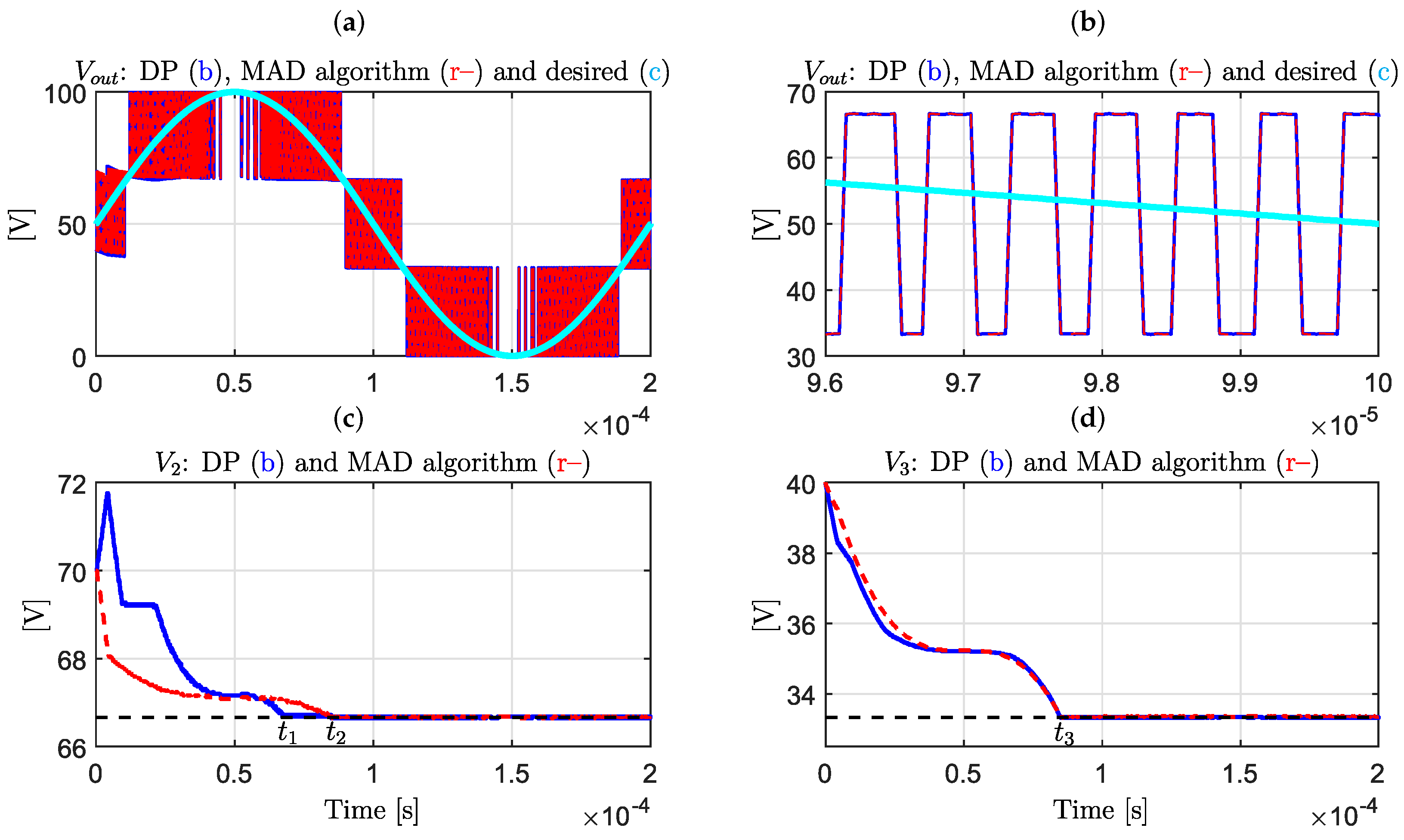
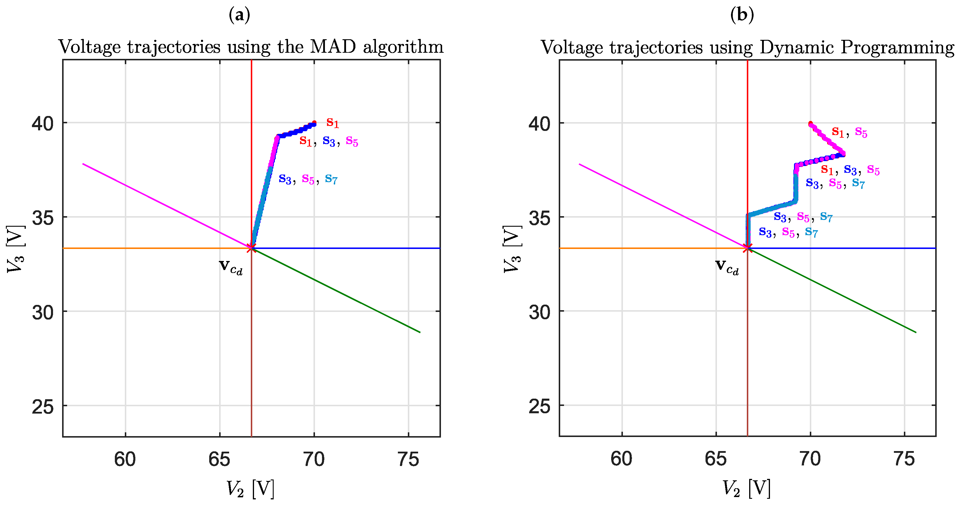
From Table 1 and from (11), in the case of $n=3$, it can be noticed that some degrees of freedom are available when the desired output voltage level L from (14) is either equal to ${\mathrm{L}}_1$ or ${\mathrm{L}}_2$:

$$\begin{array}{c}{\mathbf{T}}_j=\left\{\begin{array}{c}{\mathbf{T}}_1\hfill \\ {\mathbf{T}}_2\hfill \\ {\mathbf{T}}_4\hfill \end{array}\right.\iff {\mathbf{s}}_j=\left\{\begin{array}{c}{\mathbf{s}}_1\hfill \\ {\mathbf{s}}_2\hfill \\ {\mathbf{s}}_4\hfill \end{array}\right.\mathrm{if}\mathrm{L}={\mathrm{L}}_1,\\ {\mathbf{T}}_j=\left\{\begin{array}{c}{\mathbf{T}}_3\hfill \\ {\mathbf{T}}_5\hfill \\ {\mathbf{T}}_6\hfill \end{array}\right.\iff {\mathbf{s}}_j=\left\{\begin{array}{c}{\mathbf{s}}_3\hfill \\ {\mathbf{s}}_5\hfill \\ {\mathbf{s}}_6\hfill \end{array}\right.\mathrm{if}\mathrm{L}={\mathrm{L}}_2.\end{array}$$

(16)

Let us consider a time interval $\mathit{t}=[t_i,t_i+T_s,\dots ,t_f-T_s,t_f]$ such that

$$(\mathrm{L}\left(t_k\right)={\mathrm{L}}_1)\vee (\mathrm{L}\left(t_k\right)={\mathrm{L}}_2),\mathrm{f}\mathrm{o}\mathrm{r}\mathrm{a}\mathrm{n}\mathrm{y}{t}_k\in \mathit{t}.$$

(17)

Based on (16), a discrete-time optimal control problem that is able to guarantee that the control objectives (15) are satisfied can be written:

• For all $t_k\in \mathit{t}$ in (17),

  $$\begin{array}{c}{\displaystyle \underset{{\mathbf{s}}_j}{min}J\left({\mathbf{s}}_j\right)\mathrm{s}.\mathrm{t}.\left\{\begin{array}{l}\mathrm{a}){\dot{\mathit{V}}}_c(t_k+T_s)=\mathit{F}{\mathit{V}}_c\left(t_k\right)+\mathit{G}\mathit{u}\left(t_k\right),\\ \mathrm{b}){\mathbf{V}}_c\left(t_i\right)={\mathbf{V}}_{c_0},\\ \mathrm{c}){\mathbf{T}}_j\left(t_k\right),{\mathbf{s}}_j\left(t_k\right)\mathrm{f}\mathrm{r}\mathrm{o}\mathrm{m}\mathrm{L}\left(t_k\right)\mathrm{a}\mathrm{s}\mathrm{i}\mathrm{n}\left(16\right),\\ \mathrm{d}){\mathbf{S}}_j\left(t_k\right)\mathrm{f}\mathrm{r}\mathrm{o}\mathrm{m}{\mathbf{T}}_j\left(t_k\right)\mathrm{a}\mathrm{s}\mathrm{i}\mathrm{n}\left(3\right),\end{array}\right.}\end{array}$$

  (18)

  where the objective function $J\left({\mathbf{s}}_j\right)$ is

  $${\displaystyle J\left({\mathbf{s}}_j\right)=\sum _0^N{\left(V_2\left(t_k\right)-V_{2_d}\right)}^2+{\left(V_3\left(t_k\right)-V_{3_d}\right)}^2,}$$

and N is the length of the horizon, meaning the number of time samples $t_k\in \mathit{t}$ in (17). Points (a) and (b) in (18) describe the evolution of the capacitor voltage trajectories using the discrete-time system (7), starting from the given initial condition ${\mathbf{V}}_{c_0}$ at $t=t_i$. Points (c) and (d) in (18) describe the calculation of the components of the control versor ${\mathbf{s}}_j$ and of the configuration vector ${\mathbf{S}}_j$, affecting the capacitor voltage trajectories through the matrix $\mathbf{G}$ in system (7). The optimal control problem (18) is subject to the constraints in (16) since the desired output voltage level L needs to be generated. The objective function $J\left({\mathbf{s}}_j\right)$ in (18) to be minimized over the considered horizon N is composed of two criteria, which are the square distances of the two capacitor voltages $V_2$ and $V_3$ from the reference values $V_{2_d}$ and $V_{3_d}$ in (4). The k-th term of the objective function $J\left({\mathbf{s}}_j\right)$ in (18) is the cost of applying the control versor ${\mathbf{s}}_j\left(t_k\right)$ at $t_k=k{T}_s$. When solving optimal control problems, an established way to find the optimal control sequence that minimizes an objective function is to use dynamic programming (DP), allowing to achieve the optimal solution given by Bellman’s Principle of Optimality [40]. The principle of dynamic programming is to find the optimal control sequence by proceeding backward, therefore making the whole process much more memory efficient since it is sufficient to evaluate the arc costs at each transition occurring from the final state all the way up to the initial state. This makes this approach noncausal and not implementable in real time since it requires a priori knowledge of the converter cycle. However, DP represents the optimal benchmark that can be used as a term of comparison to evaluate the performances of the proposed MAD algorithm described in Section 3.1. An effective way of solving discrete-time constrained optimal control problems using DP is to use the dpm Matlab function [41].

4. Results

This section deals with the simulation of the MFCC in the case of $n=3$, in order to compare the results of the MAD algorithm with those of the DP optimal benchmark obtained by solving the optimal control problem in (16)–(18) using the dpm Matlab function [41]. The converter parameters used for the results of this section are shown in

Table 2. MFCC parameters and desired output voltage $V_{ou{t}_d}$.

$V_{in}$ = 100 V, $R_{in}$ = 0.1 Ω, $C_3$ = 5 μF, $C_2={\displaystyle \frac{C_3}{2}}$, $I_{out}$ = 1 A

${\displaystyle T_s}$ = 50 ns, $T_{PWM}$ = 0.6 μs, $V_{ou{t}_d}={\displaystyle \frac{V_{in}}{2}}+{\displaystyle \frac{V_{in}}{2}}sin(2\pi 5·{10}^{3}t)$

, together with the output load current that the converter is subject to and the desired output voltage waveform $V_{ou{t}_d}$, from which the desired output voltage levels L in (14) (to be provided to the MAD algorithm of Algorithm 1) can be obtained. The initial conditions of the capacitor voltages are assumed to be ${\mathbf{V}}_{c_0}={\left[\begin{array}{ccc}100& 70& 40\end{array}\right]}^T$ V, where the initial values $V_{2_0}$ and $V_{3_0}$ of the capacitor voltages $V_2$ and $V_3$ have been intentionally chosen to be different from the desired values ($V_{2_d}$ and $V_{3_d}$) given in (4); this is in order to verify the capability of the MAD control algorithm to take the reduced voltage vector ${\mathit{v}}_c={\left[\begin{array}{cc}{V}_2& V_3\end{array}\right]}^T$ back to the desired reference ${\mathit{v}}_{c_d}={\left[\begin{array}{cc}{V}_{2_d}& V_{3_d}\end{array}\right]}^T$ as quickly as possible, as required in (15). The results are shown in Figure 6, Figure 7, and

Table 3. Average efficiency, power loss, and output voltage THD.

	Average Efficiency $\overline{\mathit{E}}$	Average Power Loss ${\overline{\mathit{P}}}_{\mathit{l}}$	THD
MAD	$99.845$%	0.164 [W]	$-5.903$ [dBc]
DP	$99.850$%	0.159 [W]	$-5.903$ [dBc]

.

Figure 6a shows the desired output voltage profile $V_{ou{t}_d}$ (cyan), the output voltage values generated by the converter when controlled using DP (blue), and the MAD algorithm (red dashed). Figure 6b zooms in on the time frame $\left[9.610\right]·{10}^{-5}$ s. Figure 6c,d show the capacitor voltages $V_2$ and $V_3$ when the converter is controlled using DP (blue) and the MAD algorithm (red dashed). Regarding voltage $V_2$, it can be observed that the red dashed plot reaches the reference value (black dashed) at $t=t_2$, that is only 0.0165 ms after the time instant $t=t_1$, at which the blue plot reaches the reference value. As for voltage $V_3$, both plots reach the desired value at the same time: $t=t_3$. This proves the effectiveness of the proposed MAD algorithm, which gives convergence times that are very close or equal to those of the optimal benchmark solution while having the advantage of being implementable in real time and being comprised of very standard mathematical calculations. The colored lines in Figure 7a,b show the directions imposed on the trajectory of the reduced voltage vector ${\mathit{v}}_c={\left[\begin{array}{cc}{V}_2& V_3\end{array}\right]}^T$ by the control versors reported in Figure 3, using the same color notation, when $I_{out}<0$, as described in Remark 1. The dotted characteristics in Figure 7 show the evolution of the trajectory of the reduced voltage vector ${\mathit{v}}_c={\left[\begin{array}{cc}{V}_2& V_3\end{array}\right]}^T$ when the converter is controlled using the MAD algorithm (Figure 7a) and the DP optimal benchmark (Figure 7b). The color associated with each dot denotes the control versor ${\mathbf{s}}_j$ applied at the considered time instant $t_k$, in order to take the trajectory of the reduced voltage vector ${\mathit{v}}_c={\left[\begin{array}{cc}{V}_2& V_3\end{array}\right]}^T$ closer and closer to the desired reference ${\mathit{v}}_{c_d}$. The control versors ${\mathbf{s}}_j$ used in the different parts of the piecewise linear voltage trajectories in Figure 7 are also denoted by the colored labels “${\mathbf{s}}_j$” reported in each part of the voltage trajectories. The grey dots describing the use of control versor ${\mathbf{s}}_0$ are not visible in Figure 7 because level ${\mathrm{L}}_0$ is only required when the voltages $V_2$ and $V_3$ reach the reference values of $V_{2_d}$ and $V_{3_d}$; see Figure 6. The grey dots, therefore, accumulate around the desired reference point ${\mathit{v}}_{c_d}$. Figure 7 highlights that the MAD algorithm and DP impose different paths on the trajectory of the reduced voltage vector ${\mathit{v}}_c$, which, however, allow very similar and fast voltage convergence times, as shown in Figure 6c,d. Finally, Table 3 shows the very similar performances of the MAD algorithm and DP in terms of average efficiency $\overline{E}$ and average power loss ${\overline{P}}_l$, computed as in (2), as well as their coincident performances in terms of total harmonic distortion (THD) in the generated output voltage $V_{out}$.

In order to test the effectiveness of the MAD algorithm compared to DP in terms of capacitor voltages fast convergence, a new simulation starting from different initial capacitor voltages, lower than the desired value in this case, was performed. The results are shown in Figure 8, from which it can be seen that the convergence time $t_4$ is the same for voltages $V_2$ and $V_3$, both when using the MAD algorithm and when using the DP optimal benchmark.

5. Conclusions

In this paper, a detailed analysis of the evolution of the capacitor voltage trajectories as a function of the IGBT signals in multilevel flying-capacitor converters has led to the proposal of a new minimum angular distance algorithm. The proposed algorithm handles the turning on and off of the switches in order to achieve effective capacitor voltages balancing action while generating the desired output voltage. The proposed control algorithm is composed of very simple calculations and does not require any output current prediction. At the same time, the performance of the proposed algorithm has proven to be very good when compared with the optimal benchmark provided by dynamic programming. The future direction of this work should investigate the possible extension of the proposed algorithm to other multilevel converter topologies.

References

1. Chang, H.; Vanfretti, L. Power Hardware-in-the-Loop Smart Inverter Testing with Distributed Energy Resource Management Systems. Electronics 2024, 13, 1866. [Google Scholar] [CrossRef]
2. Cai, J.; Zhang, X.; Zhang, W.; Zeng, Y. An Integrated Power Converter-Based Brushless DC Motor Drive System. IEEE Trans. Power Electron. 2022, 37, 8322–8332. [Google Scholar] [CrossRef]
3. Zanasi, R.; Tebaldi, D. Study of the Bidirectional Efficiency of Linear and Nonlinear Physical Systems. In Proceedings of the Annual Conference of the IEEE Industrial Electronics Society, Lisbon, Portugal, 14–17 October 2019; pp. 545–552. [Google Scholar]
4. Muniandi, B.; Wan, S.; El-Yabroudi, M. Bi-Directional Charging with V2L Integration for Optimal Energy Management in Electric Vehicles. Electronics 2024, 13, 4221. [Google Scholar] [CrossRef]
5. Gómez-Ruiz, G.; Sánchez-Herrera, R.; Clavijo-Camacho, J.; Cano, J.M.; Ruiz-Rodríguez, F.J.; Andújar, J.M. A Versatile Platform for PV System Integration into Microgrids. Electronics 2024, 13, 3995. [Google Scholar] [CrossRef]
6. Alaql, F.; Alfraidi, W.; Alhatlani, A.; Al-Shamma’a, A.A.; Farh, H.M.H.; Allehyani, A. A Detailed Analysis and Gain Derivation of Reconfigurable Voltage Rectifier-Based LLC Converter. Electronics 2024, 13, 3788. [Google Scholar] [CrossRef]
7. Alouache, H.E.; Sayah, S.; Bosisio, A.; Hamouda, A.; Kouadri, R.; Shirvani, R. Optimal Placement of HVDC-VSC in AC System Using Self-Adaptive Bonobo Optimizer to Solve Optimal Power Flows: A Case Study of the Algerian Electrical Network. Electronics 2024, 13, 3848. [Google Scholar] [CrossRef]
8. Zanasi, R.; Tebaldi, D. Modeling control and robustness assessment of multilevel flying-capacitor converters. Energies 2021, 14, 1903. [Google Scholar] [CrossRef]
9. Agheb, E.; Holtsmark, N.; Høidalen, H.K.; Molinas, M. High frequency wind energy conversion system for offshore DC collection grid—Part I: Comparative loss evaluation. Sustain. Energy Grids Netw. 2016, 5, 167–176. [Google Scholar] [CrossRef]
10. Holtsmark, N.; Agheb, E.; Molinas, M.; Høidalen, H.K. High frequency wind energy conversion system for offshore DC collection grid—Part II: Efficiency improvements. Sustain. Energy Grids Netw. 2016, 5, 177–185. [Google Scholar] [CrossRef]
11. Nguyen, T.D.; Lee, H.-H. Development of a three-to-five-phase indirect matrix converter with carrier-based PWM based on space-vector modulation analysis. IEEE Trans. Ind. Electron. 2016, 63, 13–24. [Google Scholar] [CrossRef]
12. Rodrìguez, J.; Lai, J.-S.; Peng, F.Z. Multilevel inverters: A survey of topologies, controls, and applications. IEEE Trans. Ind. Electron. 2002, 49, 724–738. [Google Scholar] [CrossRef]
13. Rodrìguez, J.; Bernet, S.; Wu, B.; Pontt, J.O.; Kouro, S. Multilevel voltage-source-converter topologies for industrial medium-voltage drives. IEEE Trans. Ind. Electron. 2007, 54, 2930–2945. [Google Scholar] [CrossRef]
14. Yang, X.; Zhang, Y.; Liu, Y.; Jiang, S. Model Assisted Extended State Observer-Based Deadbeat Predictive Current Control for Modular Multilevel Converter. Electronics 2024, 13, 3789. [Google Scholar] [CrossRef]
15. Katir, H.; Abouloifa, A.; Noussi, K.; Lachkar, I.; Aroudi, A.E.; Aourir, M.; Otmani, F.E.; Giri, F. Fault tolerant backstepping control for double-stage grid-connected photovoltaic systems using cascaded H-Bridge multilevel inverters. IEEE Control Syst. Lett. 2021, 6, 1406–1411. [Google Scholar] [CrossRef]
16. Lopez, A.; Patino, D.; Diez, R.; Perilla, G. An equivalent continuous model for switched systems. Syst. Control Lett. 2013, 62, 124–131. [Google Scholar] [CrossRef]
17. Liu, M.; Li, Z.; Yang, X. A universal mathematical model of modular multilevel converter with half-bridge. Energies 2020, 13, 4464. [Google Scholar] [CrossRef]
18. Trip, S.; Cucuzzella, M.; Cheng, X.; Scherpen, J. Distributed averaging control for voltage regulation and current sharing in DC microgrids. IEEE Control Syst. Lett. 2019, 3, 174–179. [Google Scholar] [CrossRef]
19. Tebaldi, D.; Zanasi, R. Modeling Control and Simulation of a Series Hybrid Propulsion System. In Proceedings of the IEEE Vehicle Power and Propulsion Conference (VPPC), Gijon, Spain, 18 November–16 December 2020; pp. 1–7. [Google Scholar]
20. Tebaldi, D.; Zanasi, R. Systematic modeling of complex time-variant gear systems using a Power-Oriented approach. Control Eng. Pract. 2023, 132, 105420. [Google Scholar] [CrossRef]
21. Michos, G.; Baldivieso-Monasterios, P.R.; Konstantopoulos, G.C. Distributed economic nonlinear MPC for DC Micro-Grids with inherent bounded dynamics and coupled constraints. Syst. Control Lett. 2022, 167, 105327. [Google Scholar] [CrossRef]
22. Komaee, A. Optimal control with maximum cost performance measure. IEEE Control Syst. Lett. 2021, 6, 127–132. [Google Scholar] [CrossRef]
23. Ben-Brahim, L.; Gastli, A.; Trabelsi, M.; Ghazi, K.A.; Houchati, M.; Abu-Rub, H. Modular multilevel converter circulating current reduction using model predictive control. IEEE Trans. Ind. Electron. 2016, 63, 3857–3866. [Google Scholar] [CrossRef]
24. Wang, Z.; Gao, C.; Chen, C.; Xiong, J.; Zhang, K. Ripple analysis and capacitor voltage balancing of five-level hybrid clamped inverter (5L-HC) for medium-voltage applications. IEEE Access 2019, 7, 86077–86089. [Google Scholar] [CrossRef]
25. Tian, H.; Li, Y.W. Carrier-based stair edge PWM (SEPWM) for capacitor balancing in multilevel converters with floating capacitors. IEEE Trans. Ind. Appl. 2018, 54, 3440–3452. [Google Scholar] [CrossRef]
26. McGrath, B.P.; Holmes, D.G. Enhanced voltage balancing of a flying capacitor multilevel converter using phase disposition (PD) modulation. IEEE Trans. Power Electron. 2011, 26, 1933–1942. [Google Scholar] [CrossRef]
27. Kang, D.-W.; Lee, B.-K.; Jeon, J.-H.; Kim, T.-J.; Hyun, D.-S. A symmetric carrier technique of CRPWM for voltage balance method of flying-capacitor multilevel inverter. IEEE Trans. Ind. Electron. 2005, 52, 879–888. [Google Scholar] [CrossRef]
28. Moritz, R.M.B.; Batschauer, A.L. Capacitor voltage balancing in a 5-L full-bridge flying capacitor inverter. In Proceedings of the Brazilian Power Electronics Conference (COBEP), Juiz de Fora, Brazil, 19–22 November 2017. [Google Scholar]
29. Amini, J.; Abedini, A. A straightforward close-loop control strategy for a single-phase asymmetrical flying capacitor multilevel inverter. In Proceedings of the Annual International Power Electronics, Drive Systems and Technologies Conference, Tehran, Iran, 13–14 February 2013. [Google Scholar]
30. Saleh, S.A. Maximum resolution based method for balancing capacitor voltages in 7-level single phase flying-capacitor wavelet modulated inverters. IEEE Trans. Ind. Appl. 2023, 59, 5019–5031. [Google Scholar] [CrossRef]
31. Choi, S.; Saeedifard, M. Capacitor voltage balancing of flying capacitor multilevel converters by space vector PWM. IEEE Trans. Power Deliv. 2012, 27, 1154–1161. [Google Scholar] [CrossRef]
32. Borrelli, F.; Bemporad, A.; Morari, M. Predictive Control for Linear and Hybrid Systems; Cambridge University Press: Cambridge, UK, 2017. [Google Scholar] [CrossRef]
33. Ebrahimian, A.; Khan, W.A.; Weise, N. Enhanced Model Predictive Nearest Level Control for 5-Level Flying Capacitor Multilevel Converter, Hardware Implementation and Comparison. In Proceedings of the 2023 IEEE Applied Power Electronics Conference and Exposition (APEC), Orlando, FL, USA, 19–23 March 2023; pp. 2728–2734. [Google Scholar]
34. Garcia, C.; Mohammadinodoushan, M.; Yaramasu, V.; Norambuena, M.; Davari, S.A.; Zhang, Z.; Khaburi, D.A.; Rodriguez, J. FCS-MPC Based Pre-Filtering Stage for Computational Efficiency in a Flying Capacitor Converter. IEEE Access 2021, 9, 111039–111049. [Google Scholar] [CrossRef]
35. Ma, W.; Zhang, B.; Qiu, D. Robust Single-Loop Control Strategy for Four-Level Flying-Capacitor Converter Based on Switched System Theory. IEEE Trans. Ind. Electron. 2023, 70, 7832–7844. [Google Scholar] [CrossRef]
36. Bakeer, A.; Mohamed, I.S.; Malidarreh, P.B.; Hattabi, I.; Liu, L. An Artificial Neural Network-Based Model Predictive Control for Three-Phase Flying Capacitor Multilevel Inverter. IEEE Access 2022, 10, 70305–70316. [Google Scholar] [CrossRef]
37. Wang, D.; Shen, Z.J.; Yin, X.; Tang, S.; Liu, X.; Zhang, C.; Wang, J.; Rodriguez, J.; Norambuena, M. Model Predictive Control Using Artificial Neural Network for Power Converters. IEEE Trans. Ind. Electron. 2022, 69, 3689–3699. [Google Scholar] [CrossRef]
38. Ren, K.; Wang, J.; Wang, D.; He, M. Sensorless Model Predictive Control Using Artificial Neural Network for Multilevel Flying Capacitor Boost Converters. In Proceedings of the 2022 IEEE International Power Electronics and Application Conference and Exposition (PEAC), Guangzhou, China, 4–7 November 2022; pp. 1093–1097. [Google Scholar]
39. Wang, D.; Yin, X.; Tang, S.; Zhang, C.; Shen, Z.J.; Wang, J.; Shuai, Z. A Deep Neural Network Based Predictive Control Strategy for High Frequency Multilevel Converters. In Proceedings of the 2018 IEEE Energy Conversion Congress and Exposition (ECCE), Portland, OR, USA, 23–27 September 2018; pp. 2988–2992. [Google Scholar]
40. Bellman, R.E. The Theory of Dynamic Programming; The RAND Corporation: Santa Monica, CA, USA, 1954. [Google Scholar]
41. Sundstrom, O.; Guzzella, L. A generic dynamic programming Matlab function. In Proceedings of the 2009 IEEE Control Applications, (CCA) & Intelligent Control, (ISIC), St. Petersburg, Russia, 8–10 July 2009. [Google Scholar]
Figure 1. Circuital representation of the considered n-dimensional MFCC.
Electronics 14 00948 g001
Figure 2. Power-Oriented Graphs block scheme of system (1).
Electronics 14 00948 g002
Figure 3. Control versors s j for j { 0 , 1 , , 2 n 1 } on the plane ( V 2 , V 3 ) in the case of n = 3 .
Electronics 14 00948 g003
Figure 4. Block diagram of the control architecture.
Electronics 14 00948 g004
Figure 5. Example of the operation of the MAD algorithm in selecting s j when the desired output voltage level L is equal to L 1 and I o u t > 0 .
Electronics 14 00948 g005
Figure 6. Comparison between the results given by the MAD algorithm and dynamic programming: (a,b) output voltage and (c,d) capacitor voltages.
Electronics 14 00948 g006
Figure 7. Comparison between the results given by the MAD algorithm (a) and dynamic programming (b): capacitor voltage trajectories.
Electronics 14 00948 g007
Figure 8. Comparison between the results given by the MAD algorithm and dynamic programming: (a,b) capacitor voltages.
Electronics 14 00948 g008