Abstract
This paper proposes fast algorithms for odd-time and odd-frequency discrete Hartley transforms (DHTs) with normalization if the size of the input sequence ranges from 2 to 8. Fast algorithms for small-sized inputs can be included as modules in fast algorithms for discrete transforms of large-length input sequences. The existing fast odd-time DHT and odd-frequency DHT algorithms are primarily radix-type algorithms, specifically, radix-2 and prime factor algorithms. However, the algorithms in the literature do not normalize the initial transform. This means that after applying such algorithms, additional N multiplications are required. In this paper, the structural approach is exploited supposing that the starting point to design the fast algorithms is a matrix vector product expression. The factorization of the matrices of DHT coefficients is produced to reduce computational complexity taking into account the repetition and arranging of the matrix entries. The strict mathematical background proves the correctness of the obtained algorithmic solutions. Also, the MATLAB R2023b environment was applied for testing of the performance of the proposed algorithms. The obtained factorizations of the odd-time DHT and odd-frequency DHT matrices allow us to reduce the number of multiplications by 69%, while the amount of additions is decreased by about of 5% for odd-time DHTs and 8% for odd-frequency DHTs if the length of input data is in the range from 2 to 8. A comparison is provided with the direct calculation of the matrix vector product. Additionally, the computational complexity for each obtained solution is compared with the computational complexity of the existing fast algorithms for odd-time DHTs and odd-frequency DHTs. In addition, data flow graphs have been created for the proposed odd-time DHT and odd-frequency DHT algorithms. The modular space–time structure of the resulting data flow graphs is suitable for VLSI implementation.
1. Introduction
The DHT is widely applied in digital signal and image processing to obtain the frequency representation of data [1,2,3]. This transform is used in image compression [4], smart grid applications [5], wireless communication [6], audio watermarking [7], digital image watermarking [8,9,10], signal processing [11], and other applications. This transform can successfully supplement the discrete cosine transform (DCT) in different applications due to additional exploiting of the sine transform [1,2,3]. The latter allows for the processing of the signal details at high noise levels with better performance. For example, in [12], the DHT is applied in three-dimensional (3D) medical image compression. X-ray angiogram (XA) and magnetic resonance (MR) data with varied resolutions and with different numbers of frames/slices were processed. Each XA or MR data point was represented by a 3D array which was divided into blocks of size 8 × 8 × 8, and then a 3D DHT and a 3D zigzag scheme were employed. For comparison, the 3D DCT was applied with the corresponding zigzag pattern [13]. In the full 3D DHT-based codec implementation, only the first L zig-zag coefficients are preserved, encoded by entropy coding [14], and then transmitted and/or stored. However, to study the effect of the 3D DHT block, the bitrate in bit per voxel (bpv) must be calculated before entropy coding. As a result, both transforms have shown better performance at compressing XA data than MR data. Compared with the DCT on the XA data [15], approximate versions of the exact 3D DHT and the one proposed in [12] present better performance than the 3D DCT in terms of peak noise–signal ratio for the low bitrate ranging from 1 bpv to 6 bpv.
To increase robustness against various noise disturbances, similar advantages of the DHT are employed in image and audio watermarking [8,9,10]. Additionally, a significant reduction in the multiplicative complexity allows us to increase the computing efficiency and save resources [12].
To date, different DHT types have been exploited, specifically a generalized DHT [16,17], sliding DHT [18], two-dimensional DHT [19,20], 3D DHT [12], etc. However, the traditional DHT is still the most developed and researched transform compared with other types of DHT transforms [21,22,23,24]. In our paper, the odd-time DHT and odd-frequency DHT are considered. The odd-frequency DHT allows for data processing of frequencies that are centred in the range of those employed by the traditional DHT.
Direct computation of the different types of DHTs requires a huge number of arithmetic operations. Specifically, direct computation of the odd-time DHT or odd-frequency DHT of an N-point sequence requires multiplications which are especially time- and resource-consuming. To achieve a reduction in computational complexity, fast DHT algorithms have been designed [23,24,25]. But in articles devoted to the efficient implementation of the odd-time DHT and odd-frequency DHT, large-length inputs are considered [17,25,26,27,28,29,30,31]. It should be noted that more complex fast algorithms can be designed with modules containing odd-time DHT and odd-frequency DHT algorithms for short-length sequences [17]. In particular, in [21], a -point odd-frequency DHT is used to develop a split algorithm for a -point traditional DHT with reduced arithmetic complexity, where n is changed in the range from 1 to m. Once constructed, odd-time DHT and odd-frequency DHT algorithms for small-size inputs can be successfully exploited in different applications. As such, the development of fast odd-time DHT and odd-frequency DHT algorithms for short-length input sequences is a topical issue, and the appropriate approach for solving the determined parts of a general problem should be selected.
1.1. Related Papers
Most of the fast odd-time DHT and odd-frequency DHT algorithms are designed based on the divide-and-conquer strategy [17], which means obtaining a solution of a large problem via a set of solutions of smaller tasks. Bearing in mind this strategy, radix-type algorithms were developed including radix-2 and prime factor algorithms.
Thus, the radix-2 fast odd-time DHT and odd-frequency DHT algorithms were proposed in [17,26,27,28,29]. In [26,27] the proposed fast algorithms decompose the N-point odd-time DHT into two adjacent N/2-point odd-time DHTs. Such fast odd-time DHT algorithms save from 16% to 24% of the arithmetic operations in comparison with Hu’s algorithm if N varies from 16 to 64 [26].
In [17] the N-point odd-frequency DHT is decomposed into the N/2-point odd-frequency DHT and the N/2-point odd-time odd-frequency DHT. For odd-time DHT similar algorithms are also proposed. As a result, the computational complexity of the N-point odd-time DHT and odd-frequency DHT is reduced. In [28] the odd-frequency DHT of length N = was represented by several 16-point odd-frequency DHTs. Then the 16-point odd-frequency DHT is calculated by first-order moments. As a consequence, a needed number of additions and multiplications is lower than in other existing algorithms.
In [29,30] radix-2 fast algorithms are developed for the VLSI implementation of odd-time DHT and odd-frequency DHT of length N = . The algorithms differ by parallelism as well as regular and simple computational structure with low arithmetic cost.
Developed in [26,27,28,29] the fast odd-time DHT and odd-frequency DHT algorithms apply the decimation-in-frequency approach. However, for real-time applications the fast algorithms based on the decimation-in-time approach are preferable. Presented in [31] the radix-2 fast odd-time DHT algorithm with decimation-in-time substantially saves the arithmetic operations relative to Hu’s algorithm. Also, in [31] a regular signal flow graph is constructed which can be used for odd-time DHT with different lengths of inputs.
In [32] a split-radix algorithm with decimation-in-time splits N-point odd-time DHT into N/2-point odd-time DHT for even indexed samples and two odd-time DHTs of length N/4 for odd-indexed samples. Thus the number of multiplications and additions was reduced up to 29% and 10% respectively in comparison with the radix-2 odd-time DHT algorithm [31].
Mentioned radix-2 odd-time DHT and odd-frequency DHT algorithms are cost-effective but when the input sequence length is not a power of two the computational overhead frequently arises. Thus the prime factor algorithms are introduced in [17] for sequence lengths N = p × q, where p and q are relatively prime. The first prime factor algorithm decomposes the N-point odd-time DHT into p q-point odd-time DHT and q p-point odd-time DCTs. A similar decomposition also takes place for odd-frequency DHT by replacing odd-time transforms with odd-frequency transforms. However, in this case, irregularity in the index mapping occurs. To implement the in-place computation, which is easily attained by the radix-2 algorithms, the second prime factor algorithm was developed [17]. The N-point odd-time DHT is decomposed into N/q q-point odd-frequency DCTs and q N/q-point odd-time DHTs. The N-point odd-frequency DHT computation is decomposed into q N/q-point odd-frequency DHTs and N/q q-point odd-time DCTs.
Along with the algorithms synthesized based on the divide-and-conquer strategy, the algebraic signal processing is taken into account to develop the fast odd-time DHT and odd-frequency DHT algorithms. Thus, in [33] the polynomial transforms, linear congruencies, and index permutations are applied to design the fast odd-time DHT and odd-frequency DHT algorithms. In [11] fast general-radix algorithms for a wide class of orthogonal trigonometric transforms are provided. This transform class includes the odd-time DHT and odd-frequency DHTs and related algorithms are obtained by manipulating the polynomial algebras instead of manipulating the transform expression.
The short review of existing fast odd-time DHT and odd-frequency DHT algorithms has allowed defining their drawbacks and formulation of unsolved parts of the general problem of reducing computational complexity.
1.2. The Main Contributions of the Paper
After review, we note that the existing fast odd-time DHT and odd-frequency DHT algorithms are developed using polynomial algebras or radix-type approach. However, several papers devoted to fast algorithms for orthogonal trigonometric transforms exploit a structural approach that compares the transform coefficient matrix with matrix patterns [34,35,36,37,38,39]. As an option, these matrix patterns are introduced in [34] based on Winograd’s approach to the fast algorithm development. The advantage of the structural approach is the factorization of the transform matrix on sparse, scaled orthogonal, rotational, or rotational-reflection matrices [38,39]. Moreover, based on the structural approach we can obtain the data flow graphs of odd-time DHT and odd-frequency DHT algorithms with only one multiplication along the critical path [34,35,36,37]. If there is more than one multiplication in the critical path of the algorithm, then this will create additional problems for the implementation of computations.
In [37] based on the structural approach efficient algorithms for small-sized odd-time DHT were developed that do not consider the normalizing coefficients. Many authors do this, naively thinking that the result can be multiplied by the normalizing constants at subsequent stages of data processing and combined with other calculations. However, this trick cannot always be implemented, and then the normalization still has to be introduced leading to the need to perform N additional multiplications. This means that to obtain true quantitative estimates of the computational complexity of the proposed solutions, it is necessary to include N additional multiplications for each N-point algorithm, otherwise such estimates will be incorrect. To avoid such shortcomings, it is necessary to consider the normalizing constants in the original transform matrix at the very beginning.
The article [34] describes a general approach to constructing reduced complexity algorithms for calculating matrix-vector products in those cases where the matrices have certain structures. In the paper, we apply this approach to specific transforms, namely, odd-time DHT and odd-frequency DHT. Taking into account the normalization of these transforms is influenced by the number of arithmetic operations, and in some cases on the matrix structure. As a result, the mentioned approach can also allow us to obtain new interesting solutions if normalization is kept in mind.
Therefore, in this article, we consider the case of factorization of the original transformation matrices, the entries of which are already initially multiplied by the corresponding normalizing constants. This paper aims to reduce the computational complexity of the odd-time DHT and odd-frequency DHT with normalization via developing fast algorithms. We base on the structural approach supposing that input sequence length N is changed from 2 to 8.
The article is organized as follows. The considered problem is introduced and the research subject is formulated in Section 1. Brief mathematical background is provided and the used notations are defined in Section 2. Section 3 is devoted to odd-time DHT and odd-frequency DHT matrix factorizations for different N from 2 to 8 and following obtaining of the fast odd-time DHT and odd-frequency DHT algorithms via the data flow graphs. In Section 4 and Section 5 the computational complexity of the proposed fast odd-time DHT and odd-frequency DHT algorithms is evaluated. In Section 6 the conclusions are provided.
2. Preliminary Background
The traditional DHT is expressed as follows [17]:
where casθ = sinθ + cosθ = cos(θπ/4); is the output data sequence after the traditional DHT; is the sequence of input data; N is the number of signal samples.
The direct generalized DHT can be described by the following expression [17]:
where is the output sequence after the direct generalized DHT; is a time shift; is a frequency shift.
Using the expression (2) we have the traditional DHT if the odd-time DHT if the odd-frequency DHT if the odd-time odd-frequency DHT if When for the odd-time DHT with normalization the expression (2) is represented as follows [17]:
where is the output sequence after the odd-time DHT.
For the odd-frequency DHT with normalization we derive the expression (2) as follows [17]:
where is the odd-frequency DHT outputs, .
The odd-time DHT and odd-frequency DHT can be obtained as a matrix-vector product:
where , for odd-time DHT, and for odd-frequency DHT, n, k = 0, …, N − 1; , .
Because the generalized DHT with normalization is orthonormal then the matrices of inverse transforms are transposed to the direct ones. That is, for odd-time DHT the inverse is odd-frequency DHT and vice versa. For traditional DHT the inverse transform is the same [40].
In the article the following notations and abbreviations are used [34]:
- ⊕ is the direct sum of two matrices;
- is an order N identity matrix;
- ⊗ is a Kronecker product of two matrices;
- is a 2 × 2 Hadamard matrix;
- is a multiplier;
- is a permutation matrix;
- is a block-diagonal matrix of size M × N;
- , are block-diagonal and diagonal matrices of size N × N, respectively;
- an empty cell in a matrix means that it contains zero;
- DHT is a discrete Hartley transform;
- VLSI is very large-scale integration;
- DCT is a discrete cosine transform;
- XA is a X-ray angiogram;
- MR is magnetic resonance;
- 3D is a three-dimensional data.
3. Reduced Complexity Algorithms for Short-Length Odd-Time DHT and Odd-Frequency DHT
3.1. Algorithms for 2-Point Odd-Time DHT and Odd-Frequency DHT
To develop the algorithm for two-point odd-time DHT with normalization we consider the expression:
where , 0.7071, 0.7887, 0.2113, , . The expression (6) for two-point odd-frequency DHT with normalization is the same because .
Then the factorization of the odd-time and odd-frequency DHT matrix for N = 2 can be presented as follows:
where .
We have shown a data flow graph of the algorithm for the 2-point odd-time DHT and odd-frequency DHT in Figure 1. As can be seen, we have 2 additions as well as when using the direct method. The number of multiplication is also 2 against 4 multiplications for the direct matrix-vector product.
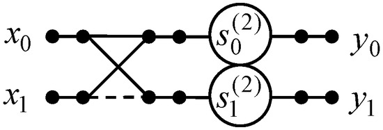
Figure 1.
The data flow graph of the proposed algorithm for computation of two-point odd-time DHT and odd-frequency DHT.
3.2. Algorithms for 3-Point Odd-Time DHT and Odd-Frequency DHT
The expression for 3-point odd-time DHT with normalization is as follows:
where , , with 0.5774, 0.7887, 0.2113. For odd-frequency DHT with normalization we use instead of in Equation (8).
To factorize the matrix we swap the first and second rows. Then we alter the sign of the third row and third column of the resulted matrix and decompose it into two components:
where , .
In the second column and second row of the matrix we obtained identical entries that differ only in sign. Therefore, the number of operations can be reduced without additional transforms. Next, we eliminate the second row and second column containing only zero entries in matrix , and matrix was obtained.
We derive the factorization for the 3-point odd-time DHT based on the decomposition of matrix [34,37]:
where , , , ,
Based on Equation (10) the factorization for the 3-point odd-frequency DHT is obtained as:
A data flow graph of the 3-point odd-time DHT algorithm is shown in Figure 2. Then the amount of multiplications can be reduced from 9 to 3 because . However, the number of additions enlarges from 6 to 7.
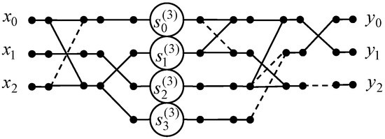
Figure 2.
The data flow graph of the algorithm for the 3-point odd-time DHT.
A data flow graph of the 3-point odd-frequency DHT algorithm is shown in Figure 3. The number of arithmetic operations remains the same as for 3-point odd-time DHT.
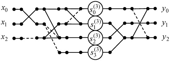
Figure 3.
The data flow graph of the algorithm for the 3-point odd-frequency DHT.
3.3. Algorithms for 4-Point Odd-Time DHT and Odd-Frequency DHT
The four-point odd-time DHT with normalization is defined as follows:
where , , with 0.5, 0.7071. For odd-frequency DHT with normalization we use instead of in Equation (12).
We permutate the rows of according to . The permutation matrix is . The obtained matrix matches the pattern where and .
Applying the matrix templates from [34,37], we derive the expressions
Therefore the factorization of the 4-point odd-time DHT matrix is as follows:
where , , .
The data flow graph of the 4-point odd-time DHT algorithm is presented in Figure 4. As one can see, the number of multiplications is reduced from 4 to 2 because , the number of additions is decreased from 8 to 6 compared to direct matrix-vector product.
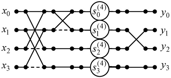
Figure 4.
The data flow graph of the algorithm for implementation of 4-point odd-time DHT.
Taking into consideration the Equation (14), the factorization for the four-point odd-frequency DHT matrix is expressed as
The algorithm of the 4-point odd-frequency DHT with normalization is provided as a data flow graph in Figure 5. The number of arithmetic operations is the same as for odd-time DHT.
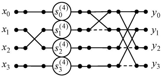
Figure 5.
The data flow graph of the algorithm for implementation of 4-point odd-frequency DHT.
3.4. Algorithms for 5-Point Odd-Time DHT and Odd-Frequency DHT
To develop the algorithm for five-point odd-time DHT with normalization we use the following expression
where , , = 0.4472, =0.6247, = 0.2871, = 0.5635, = 0.0989,
For odd-frequency DHT with normalization in Equation (16) we use instead of .
We alter the order of rows and columns of applying the permutations
The corresponding permutation matrices are as follows
Then we decompose the resulting matrix into two submatrices:
where and .
In the third column and third row of the matrix it is obtained identical entries that differ only in sign. Therefore, the number of operations can be reduced without additional transforms [36]. We eliminate in matrix the row and column with only zero entries. The resulted matrix
matches the matrix template where , .
The factorization of template is known from [34], and we represent the matrix as
where . The resulting matrices and match the templates and , respectively. Therefore, we obtain the following factorizations from [34]:
where , g h p q
Let us add matrices from decomposition (19) to the left of the diagonal matrix into the matrix , and to the left of the diagonal matrix into the matrix . Combining the expressions (17), (18), and (19) the matrix factorization for the five-point odd-time DHT with normalization is represented as
where
We have added the matrix into the crossing of third and fourth columns and rows of the matrices , and . This allows the factorizing the matrix using and .
Next, we present the algorithm of the five-point odd-time DHT with normalization via the data flow graph in Figure 6. As one can see, the number of multiplications is reduced from 25 to 6 because ; the number of additions is enlarged from 20 to 23.
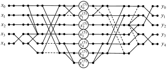
Figure 6.
The data flow graph of the algorithm for the 5-point odd-time DHT.
Based on Equation (20), the matrix factorization for the five-point odd-frequency DHT with normalization is represented as
Figure 7 shows a data flow graph of the algorithm for the five-point odd-frequency DHT with normalization. The number of arithmetic operations is the same as for 5-point odd-time DHT with normalization.
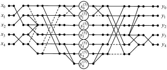
Figure 7.
The data flow graph of the algorithm for the 5-point odd-frequency DHT.
3.5. Algorithms for 6-Point Odd-Time DHT and Odd-Frequency DHT
Let us propose an algorithm for six-point odd-time DHT with normalization which is expressed as follows:
where , ,
with = 0.5577, = 0.1494. For odd-frequency DHT with normalization in Equation (22) we use instead of .
Note that = , thus we decompose , where
Further the matrix is added to factorization immediately as a submatrix of the matrix : , . The matrix is determined by the structure of the matrix for which the second and sixth rows, the third and fifth rows are the same except on the sign. The matrices and will denote the order of the columns and the rows of the matrices and in resulted factorization. The identity submatrix of and related to , and the rest submatrices of and related to :
Let us introduce to multiply the each row of matrix , and to multiply the each row of . Then the factorization of the matrix of the 6-point odd-time DHT with normalization can be expressed as [37]
where .
Figure 8 shows the data flow graph of the algorithm of the 6-point odd-time DHT with normalization. The amount of multiplications and additions can be lessened from 36 to 8 and from 30 to 28, respectively.
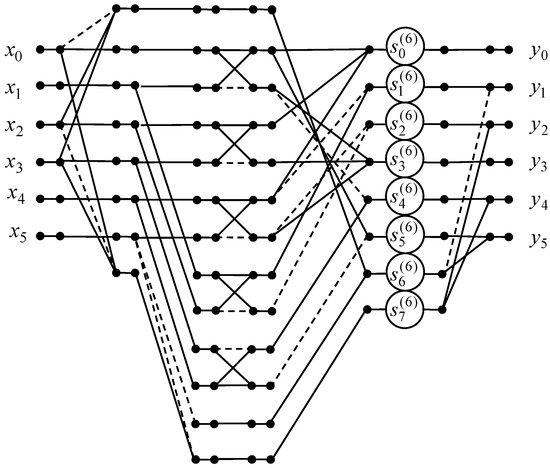
Figure 8.
The data flow graph of the algorithm for the computation of the 6-point odd-time DHT.
Based on Equation (23), the matrix factorization for the 6-point odd-frequency DHT with normalization is expressed as
Figure 9 shows the data flow graph of the algorithm implementing the 6-point odd-frequency DHT with normalization. As one can see, the amount of multiplications may be lessened from 36 to 8. Also we decreased the amount of additions from 30 to 24.
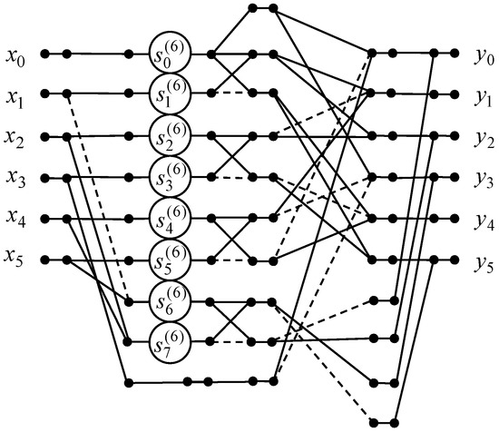
Figure 9.
The data flow graph of the algorithm for the computation of the 6-point odd-frequency DHT.
3.6. Algorithms for 7-Point Odd-Time DHT and Odd-Frequency DHT
Now we will design the algorithm for 7-point odd-time DHT with normalization using the expression
where , , = 0.3780, = 0.5045, = 0.4526, = 0.0598, = 0.5312, = 0.1765, = 0.2844,
For odd-frequency DHT with normalization in Equation (25) the matrix must be used instead of .
Let us define the permutations and :
After permutation of the rows of with and permutation the columns of with , we alter the sign of the fifth, sixth, and seventh columns. The corresponding permutation matrices are introduced as
The obtained matrix was decomposed into two components:
where
We can reduce the number of operations by taking into account the similar entries in the fourth column and fourth row of the matrix [36], which differ only in sign. Next, in matrix we eliminate the rows and columns with only zero entries. The obtained matrix
acquires the structure and can be decomposed as [34]:
Now we will decompose the matrices
representing them as a circular convolution matrix [35,36]:
where ; ,
We need to modify the matrices , to make them consistent with the expression of the circular convolution for N = 3. For that, in the matrix the sign of entries in the first column and first row was altered by multiplying left and right on . In the matrix the sign of the second-row entries was changed by multiplying left on . As a result, we obtain the matrices:
Let us apply the expression (28) to , For the matrix the elements of circular convolution are . For the matrix we have . Further we form the matrices , to factorize the circular convolutions. The matrices and were multiplied on and . And we obtained , ,
We have added the matrix into direct sum in the matrices , and . This allows the factorizing the matrix using and .
In sum, we derive the factorization of the matrix of the seven-point odd-time DHT with normalization:
where ,
To calculate the 7-point odd-time DHT with normalization the fast algorithm is developed and presented in Figure 10 by data flow graph. As a consequence we can reduce the amount of multiplications from 49 to 10, but the amount of additions increased from 42 to 46.
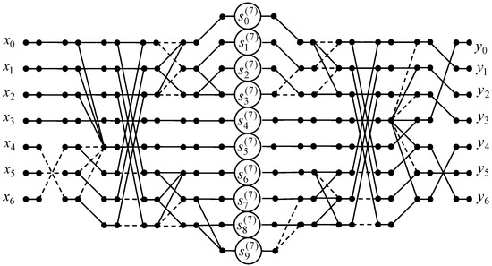
Figure 10.
The data flow graph implementing the 7-point odd-time DHT.
Based on Equation (29), the matrix factorization for the 7-point odd-frequency DHT with normalization is obtained as
To compute the 7-point odd-frequency DHT with normalization we propose the fast algorithm shown in Figure 11 by data flow graph. The number of arithmetic operations is the same as for 7-point odd-time DHT with normalization.
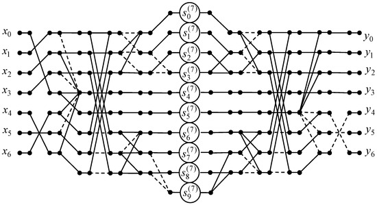
Figure 11.
The data flow graph implementing the 7-point odd-frequency DHT.
3.7. Algorithms for 8-Point Odd-Time DHT and Odd-Frequency DHT
Let us develop the algorithm for eight-point odd-time DHT with normalization which is expressed as follows:
where , ,
with = 0.3536; = 0.4619; = 0.1913; = 0.5. For odd-frequency DHT with normalization in (31) the matrix must be used instead of .
Let us define the permutation to change the order of rows of . The permutation matrix and the resulted matrix can be expressed as
The resulted matrix acquires the structure:
Then using the template from [34] we obtain . The matrix has the following structure:
Using the decomposition of the extracted submatrices [34], the matrix is represented as
The entries of the diagonal matrix we denoted as
Next we swap the first and second column of the matrix with permutation matrix . The resulted matrix is similar to the template and can be decomposed as
where matches the pattern , , . It is represented as
where , are defined as in Equation (19). The entries of diagonal matrix we denoted as The matrix is similarly decomposed with diagonal matrix entries
Let us add matrices from decomposition (34) to the left of the diagonal matrix into the matrix , and to the right of the diagonal matrix into the matrix . Also we added matrices from decompositions (32), (33) to the left of the diagonal matrices into the matrix , and to the right of the diagonal matrices into .
In sum, the 8-point odd-time DHT with normalization is factorized as
where .
To compute the 8-point odd-time DHT with normalization the data flow graph of the fast algorithm is designed and presented in Figure 12. As a consequence we can reduce the amount of multiplications from 48 to 8, because , and the amount of additions from 48 to 28.
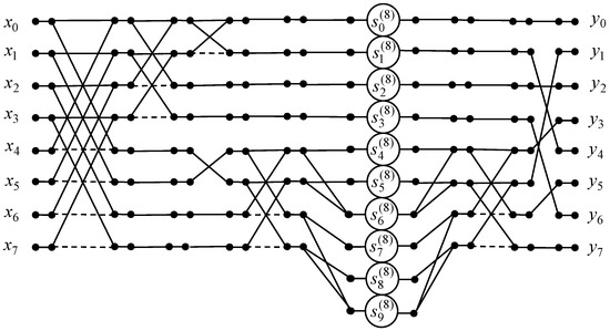
Figure 12.
The data flow graph for the computing of the 8-point odd-time DHT.
Based on Equation (35), the matrix factorization for the 8-point odd-frequency DHT with normalization is given as
Figure 13 shows the data flow graph of the algorithm implementing the 8-point odd-frequency DHT with normalization. The amount of arithmetic operations is the same as for 8-point odd-time DHT with normalization.
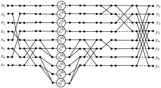
Figure 13.
The data flow graph of the algorithm for the 8-point odd-time DHT.
4. Results
We confirmed the correctness of the odd-time DHT and odd-frequency DHT matrix factorizations obtained in Section 3 by experiment. Using the MATLAB R2023b software it was evaluated the coincidence of the results of the multiplication of factorized matrices by Formulas (7), (10), (14), (20), (23), (29), and (35) with the original odd-time DHT matrices. Also, it was evaluated the similarity of the results of the computing of the matrices of the odd-frequency DHT with the expressions (11), (15), (21), (24), (30), (36) using the MATLAB R2023b environment. The last formulas define the factorizations of the odd-frequency DHT matrices. The obtained coincidence of the factorized matrices with the initial odd-time DHT and odd-frequency DHT matrices for each N indicates the correctness of the developed algorithms.
Next, we evaluated the number of arithmetic operations for the calculation of the odd-time DHT and odd-frequency DHT with normalization via matrix-vector product and for the proposed algorithms. In general, the multiplications on data flow graphs are corresponded to the graph vertices, denoted by circles with factors. The amount of additions was evaluated by the amount of entering of two graph edges in one vertex. One must notice that these operations for zero elements of odd-time DHT and odd-frequency DHT matrices were not counted. In the matrices and we have four and eight zeros, respectively. Also if an element of the odd-time DHT or odd-frequency DHT matrix can be expressed as a power of two then the multiplication by this element can be implemented by a shift and has not counted as a multiplication. The proposed algorithms use the same number of multiplications to both the odd-time DHT and the odd-frequency DHT with normalization. Applying these algorithms we can reduce the number of multiplications required for odd-time or odd-frequency DHTs by nearly 69%, and the amount of additions by nearly of 5% for odd-time DHT and 8% for odd-frequency DHT if the length of input data is in the range from 2 to 8.
Table 1 shows the obtained results. In parentheses, we indicate the difference in the amount of operations in percent. The plus means that the amount of operations has increased relative to the matrix-vector product, and the minus means it has lessened. In Table 2 and Table 3 the number of multiplication and additions is presented for the existing odd-time DHT and odd-frequency DHT algorithms.

Table 1.
The computational complexity of the matrix-vector product and the proposed fast algorithms for odd-time and odd-frequency DHTs.
Table 2.
The number of operations for the existing odd-time DHT algorithms.
Table 3.
The number of operations of the existing odd-frequency DHT algorithms.
5. Discussion of Computational Complexity
Let us compare the number of multiplication and additions for the existing algorithms and for the proposed algorithms of odd-time DHT and odd-frequency DHT with normalization. As for the odd-time DHT, if N = 4 then the proposed algorithm is no different from algorithms known from the literature by the multiplication number. However if the existing algorithms do not include the normalization they require the additional four multiplications. If N = 8 then the amount of multiplications may be lessened with the proposed solution versus Hamood’s algorithms [31,32] by 33%. Relative to the prime factor algorithm [17], the amount of multiplications for N = 8 is the same, and less than for the radix-2 algorithm [27] by 20%. However, the considered existing algorithms of odd-time DHT do not include normalization for N = 8 which requires 8 additional multiplications. The amount of additions for N = 8 has increased by 17% relative to Hamood’s algorithms [31,32] and is the same as for algorithms in [17,27].
As for the odd-frequency DHT, if N = 4 then the obtained algorithm is no different from algorithms known from the literature by the amount of multiplications. However the absence of normalization requires the additional four multiplications. Besides, for N = 4, the proposed algorithm reduces the number of additions significantly (by 40–45%). If N = 8 then the number of multiplications may be significantly lessened with the proposed solution relative to the radix-2 algorithm [28,29] but exceeds by 33% the number of multiplications for the algorithm of the prime factor (N = ) without normalization [17,41,42]. The normalization will require 8 additional multiplications.
Due to the evaluation that has been done in [34], we can estimate the reduction of computational complexity of the proposed algorithms by Big O notation. The list represents the number of arithmetic operations that the algorithm performs to obtain the odd-time or odd-frequency DHT of size N. We can use the estimation of template complexity for even N directly. For odd N we have decomposed the initial transform matrix as the sum of two matrices. Therefore we have to add two multiplications and 2(N − 1) additions to the Big O notation of the template complexity. The obtained estimations are summarised in Table 4. Analysing the resulting Big O estimates it should be noted the following. The number of multiplications is reduced two times, in general, although the number of additions is increased by 2(N − 1) if the proposed algorithms are compared to the direct matrix-vector product.
Table 4.
The computational complexity of the proposed algorithms and the direct matrix-vector product in the Big O notation.
6. Conclusions
In the paper, the fast algorithms for odd-time DHT and odd-frequency DHT with normalization are proposed for input signals of short length. The obtained algorithms for short-length input signals can subsequently be used as readymade modules of algorithms for long-length sequences.
Including the normalization in the fast algorithms for odd-time DHT and odd-frequency DHT allows us to use them directly in applications that involve recovering the processed signals or images, specifically, in image compression, signal and image denoising, image encryption, etc. Normalization ensures the orthonormality of transform and, as a result, the inverse transform matrix is obtained by a transposing of the direct transform matrix. The last property enables the construction of fast algorithms for inverse transform based on the fast algorithms for direct transform easily.
The fast algorithms for odd-time DHT and odd-frequency DHT were developed in the article based on the structural properties of the matrices of the transform coefficients. Optimization of the parameters of the odd-time DHT and odd-frequency DHT is not performed. We have applied the partition of the initial matrix into the submatrices with previous rearranging of the matrix rows and/or columns. The partitioning of the original matrix and rearranging its structure aims to find the factorization which possibly reduces further the computational complexity. Based on the obtained factorizations, we have constructed the fast algorithms presented by the data flow graphs. The critical path of each designed data flow graph has only one multiplication. This is a significant advantage of the proposed solutions. If the critical path of the data flow graph has more than one multiplication, additional difficulties arise with the presentation and further processing of the result of each successive multiplication.
The comparison of the computational complexity of the direct matrix-vector products with the computational complexity of the proposed algorithms has shown a reducing in the number of multiplications by 69% for the input sequence lengths from 2 to 8. At the same time, the amount of additions is lowered by nearly 5% for odd-time DHT and by 8% for odd-frequency DHT for the same range of the input sequence lengths.
The comparison of the designed fast algorithms for odd-time DHT and odd-frequency DHT with the existing algorithms shows that bearing in mind the structure of transform matrices enabled the increase in the fast algorithms’ efficiency against the efficiency of radix-type algorithms. This result enables easier operation in real time because the amount of needed signal processor resources is significantly reduced. Reducing the number of multiplications significantly contributes to the resource- and time-saving of signal processing and enables easier operation in real-time.
Author Contributions
Conceptualization, A.C.; methodology, A.C. and M.P.; software, M.P.; validation, A.C., M.P. and J.S.; formal analysis, A.C., M.P. and J.S.; investigation, M.P. and J.S.; writing—original draft preparation, M.P. and A.C.; writing—review and editing, A.C., M.P. and J.S.; supervision, A.C. All authors have read and agreed to the published version of the manuscript.
Funding
This research received no external funding.
Data Availability Statement
Data are contained within the article.
Conflicts of Interest
The authors declare no conflicts of interest. The funders had no role in the design of the study; in the collection, analyses, or interpretation of data; in the writing of the manuscript; or in the decision to publish the results.
References
- Jones, K. The regularized fast Hartley transform. In Low-Complexity Parallel Computation of the FHT in One and Multiple Dimensions, 2nd ed.; Springer: New York, NY, USA, 2021. [Google Scholar]
- Patra, N.; Nayak, S.S. Discrete Hartley transform and its applications—A review. J. Integr. Sci. Technol. 2022, 10, 173–179. [Google Scholar]
- Moraga, C. Generalized discrete Hartley transforms. In Proceedings of the 39th International Symposium on Multiple-Valued Logic, Naha, Japan, 21–23 May 2009. [Google Scholar]
- Vimal Kumar, C.; Raghavendra, D.; Eshwarappa, M.N. Design and implementation of VLSI DHT algorithm for image compression. Int. J. Eng. Trends Technol. 2015, 23, 218–223. [Google Scholar] [CrossRef]
- de Oliveira Nascimento, F.A. Hartley transform signal compression and fast power quality measurements for smart grid application. IEEE Trans. Power Deliv. 2023, 99, 1–11. [Google Scholar] [CrossRef]
- Anoh, K.; Tanriover, C.; Ribeiro, M.V.; Adebisi, B.; See, C.H. On the fast DHT precoding of OFDM signals over frequency-selective fading channels for wireless applications. Electronics 2022, 11, 3099. [Google Scholar] [CrossRef]
- Budiman, G.; Suksmono, A.B.; Danudirdjo, D.; Pawellang, S. QIM-based audio watermarking with combined techniques of SWT-DST-QR-CPT using SS-based synchronization. In Proceedings of the 6th International Conference on Information and Communication Technology (ICoICT), Bandung, Indonesia, 3–4 May 2018. [Google Scholar]
- Lipinski, P.; Puchala, D. Digital image watermarking using fast parametric transforms. Bull. Pol. Acad. Sci. Tech. Sci. 2019, 67, 463–477. [Google Scholar] [CrossRef]
- Kasban, H. A spiral-based image watermarking scheme using Karhunen–Loeve and discrete Hartley transforms. Multidimens. Syst. Signal Process. 2017, 28, 573–595. [Google Scholar] [CrossRef]
- Zhang, X.; Su, Q. A spatial domain-based colour image blind watermarking scheme integrating multilevel discrete Hartley transform. Int. J. Intell. Syst. 2021, 36, 4321–4345. [Google Scholar] [CrossRef]
- Voronenko, Y.; Puschel, M. Algebraic Signal Processing Theory: Cooley-Tukey Type Algorithms for Real DFTs. IEEE Trans. Signal Process. 2009, 57, 205–222. [Google Scholar] [CrossRef]
- Coutinho, V.A.; Cintra, R.J.; Bayer, F.M. Low-complexity three-dimensional discrete Hartley transform approximations for medical image compression. Comput. Biol. Med. 2021, 139, 105018. [Google Scholar] [CrossRef]
- Bozinovic, N.; Konrad, J. Scan order and quantization for 3D-DCT coding. Proc. SPIE Vis. Commun. Image Process. 2003, 5150, 1205. [Google Scholar]
- Rao, K.R.; Yip, P. The Transform and Data Compression Handbook, 1st ed.; CRC Press LLC: Boca Raton, FL, USA, 2001. [Google Scholar]
- Rao, K.R.; Yip, P. Discrete Cosine Transform: Algorithms, Advantages, Applications, 2nd ed.; Academic Press: Cambridge, UK, 2014. [Google Scholar]
- Prots’ko, I. Algorithm of efficient computation of generalised discrete Hartley transform based on cyclic convolutions. IET Signal Process. 2014, 8, 301–308. [Google Scholar] [CrossRef]
- Bi, G.; Zeng, Y. Transforms and Fast Algorithms for Signal Analysis and Representations, 1st ed.; Birkhäuser: Boston, FL, USA, 2004. [Google Scholar]
- Kober, V. Fast recursive computation of sliding DHT with arbitrary step. Sensors 2020, 20, 5556. [Google Scholar] [CrossRef]
- Jiang, L.; Shu, H.; Wu, J.; Wang, L.; Senhadji, L. A novel split-radix fast algorithm for 2-D discrete Hartley transform. IEEE Trans. Circuits Syst. I Regul. Pap. 2010, 57, 911–924. [Google Scholar] [CrossRef]
- Wu, J.; Shu, H.; Senhadji, L.; Luo, L.M. Radix-3x3 algorithm for the 2-D discrete Hartley transform. IEEE Trans. Circuits Syst. Part 2 Analog Digit. Signal Process. 2008, 55, 566–570. [Google Scholar]
- Grigoryan, A.M. Novel algorithm for computing the 1-D discrete Hartley transform. IEEE Signal Process. Lett. 2004, 11, 156–159. [Google Scholar] [CrossRef]
- Hamood, M. New efficient algorithm for the discrete Hartley transform. IOP Conf. Ser. Mater. Sci. Eng. 2020, 978, 012013. [Google Scholar] [CrossRef]
- Chiper, D.F. A novel VLSI DHT algorithm for a highly modular and parallel architecture. IEEE Trans. Circuits Syst. II Express Briefs 2013, 60, 282–286. [Google Scholar] [CrossRef]
- Pyrgas, L.; Kitsos, P.; Skodras, A.N. An FPGA design for the two-band fast discrete Hartley transform. In Proceedings of the IEEE International Symposium on Signal Processing and Information Technology (ISSPIT), Limassol, Cyprus, 12–14 December 2016. [Google Scholar]
- Yang, X.; Megson, G.M.; Xing, Y.; Evans, D.J. A novel radix-3/9 algorithm for type-III generalized discrete Hartley transform. J. Circuits Syst. Comput. 2006, 15, 301–312. [Google Scholar] [CrossRef]
- Shu, H.; Wang, Y.; Senhadji, L.; Luo, L. Direct computation of type-II discrete Hartley transform. IEEE Signal Process. Lett. 2007, 14, 329–332. [Google Scholar] [CrossRef][Green Version]
- Chiper, D.F. Fast radix-2 algorithm for the discrete Hartley transform of type II. IEEE Signal Process. Lett. 2011, 18, 687–689. [Google Scholar] [CrossRef]
- Hua, X.; Liu, J. A novel fast algorithm for discrete Hartley transform of type-III base on the split-radix and first-order moments. In Proceedings of the SPIE Eighth International Symposium on Multispectral Image Processing and Pattern Recognition, Wuhan, China, 26–27 October 2013. [Google Scholar]
- Chiper, D.F. Radix-2 fast algorithm for computing discrete Hartley transform of type III. IEEE Trans. Circuits Syst. II Express Briefs 2012, 59, 297–301. [Google Scholar] [CrossRef]
- Chiper, D.F. An improved algorithm for the VLSI implementation of type II generalized DHT that allows an efficient incorporation of obfuscation technique. In Proceedings of the 45th International Conference on Telecommunications and Signal Processing (TSP), Prague, Czech Republic, 13–15 July 2022. [Google Scholar]
- Hamood, M.T. Fast algorithm for computing the discrete Hartley transform of type-II. Indones. J. Electr. Eng. Inform. 2016, 4, 120–125. [Google Scholar] [CrossRef]
- Hamood, M.T. Direct split-radix algorithm for fast computation of type-II discrete Hartley transform. Telecommun. Comput. Electron. Control 2020, 18, 3067–3072. [Google Scholar] [CrossRef]
- Huang, Y.-M.; Wu, J.-L. Polynomial transform based algorithms for computing two-dimensional generalized DFT, generalized DHT, and skew circular convolution. Signal Process. 2000, 80, 2255–2260. [Google Scholar] [CrossRef]
- Cariow, A. Strategies for the synthesis of fast algorithms for the computation of the matrix-vector product. J. Signal Process. Theory Appl. 2014, 3, 1–19. [Google Scholar] [CrossRef]
- Cariow, A.; Papliński, J. Algorithmic structures for realizing short-length circular convolutions with reduced complexity. Electronics 2021, 10, 2800. [Google Scholar] [CrossRef]
- Polyakova, M.; Witenberg, A.; Cariow, A. The design of fast type-V discrete cosine transform algorithms for short-length input sequences. Electronics 2024, 13, 4165. [Google Scholar] [CrossRef]
- Polyakova, M.; Cariow, A. Fast Type-II Hartley Transform Algorithms for Short-Length Input Sequences. Appl. Sci. 2024, 14, 10719. [Google Scholar] [CrossRef]
- Perera, S.M. Signal flow graph approach to efficient and forward stable DST algorithms. Linear Algebra Its Appl. 2018, 542, 360–390. [Google Scholar] [CrossRef]
- Perera, S.M.; Lingsch, L. Sparse matrix-based low-complexity, recursive, radix-2 algorithms for discrete sine transforms. IEEE Access 2021, 9, 141181–141198. [Google Scholar] [CrossRef]
- Paraskevas, I.; Barbarosou, M.; Chilton, E. Hartley transform and the use of the whitened Hartley spectrum as a tool for phase spectral processing. J. Eng. 2015, 2015, 95–101. [Google Scholar] [CrossRef]
- Wang, Z. A prime factor fast W transform algorithm. IEEE Trans. Signal Process. 1992, 40, 2361–2368. [Google Scholar] [CrossRef] [PubMed]
- Hu, N.C.; Chang, H.I.; Ersoy, O.K. Generalized discrete Hartley transforms. IEEE Trans. Signal Process. 1992, 40, 2931–2940. [Google Scholar]


Disclaimer/Publisher’s Note: The statements, opinions and data contained in all publications are solely those of the individual author(s) and contributor(s) and not of MDPI and/or the editor(s). MDPI and/or the editor(s) disclaim responsibility for any injury to people or property resulting from any ideas, methods, instructions or products referred to in the content. |
© 2025 by the authors. Licensee MDPI, Basel, Switzerland. This article is an open access article distributed under the terms and conditions of the Creative Commons Attribution (CC BY) license (https://creativecommons.org/licenses/by/4.0/).