Development of an IoT-Enabled Smart Electricity Meter for Real-Time Energy Monitoring and Efficiency

Abstract

Smart meters play an important role in energy management systems as they provide essential parameters for real-time monitoring, protection, and control that enable informed decisions for the end-users and the utility grid. However, available systems are high-cost solutions with different hardware and software, which provide limited measuring parameters with certain accuracy. This work aims to develop and implement an innovative smart electricity meter (SEM) system that surpasses conventional designs by incorporating advanced features like noninvasive sensors, manual signal calibration, and flexible communication modes. The developed SEM supports real-time data transmission via IoT and provides superior accuracy in measuring harmonics and frequency, addressing key challenges in energy monitoring. This work contributes to real-time energy monitoring and energy management systems in residential and industrial applications.

1. Introduction

Optimizing energy use is a global priority, as reflected in the United Nations Sustainable Development Goals (SDGs), particularly those addressing affordable and clean energy (SDG 7) [1]. In Chile, energy efficiency law N°21.305 promotes the implementation of energy management systems (EMS) for large consumers (with annual consumption above 50 Tcal), underscoring the crucial need to improve energy efficiency and reduce overall consumption [2]. Smart energy meters (SEMs) are key enablers of such efficiency improvements, as they provide essential measurements for managing energy in generation, transmission, and distribution [3,4,5]. Beyond monitoring variables like active and reactive power, load current, and voltage, they can also track parameters such as frequency, total harmonic distortion (THD), and RMS values, boosted by advanced signal processing and data fusion at embedded systems level electronics [6]. Technological advances in energy digitalization based on the Internet of Things (IoT), cyber-physical systems (CPS), sensor fusion, and data analytics enable more intelligent energy monitoring and control [7]. For instance, deploying IoT in SEMs allows real-time data transfer, supporting advanced functionalities like remote switching, data analysis, and integration with renewable energies [8,9]. This evolution supports greenhouse gas emissions reduction and optimizes energy management [10,11,12]. Furthermore, digitalization has led to significant growth in the use of SEMs. Between 2010 and 2019, the number of installed SEMs worldwide increased from 23.5 million to approximately 729.1 million, revealing a massive surge in demand for more accurate and connected meters [13].

There are many related works that have addressed SEM from different perspectives, such as the number of measuring parameters, types of sensor nodes, and the selection of hardware/software [14,15,16,17,18,19,20,21,22,23,24,25,26,27]. However, the majority of such works are lacking important measurements such as harmonics, THD, and frequency, as well as other features such as manual calibration, remote control, and the support of different communication technologies. To address such a knowledge gap, this work aims to design and implement an SEM for real-time monitoring, featuring signal calibration and flexible communication that enables an informed decision for the end-user for real-time monitoring, protection, and control.

The main contribution of this work is the design of an SEM for an efficient energy management technology. The main feature of SEM is the measurement of electrical variables not available in conventional market sensors (harmonics, THD, and frequency). Besides, additional features of the SEM are the fusion of IoT technology, use of a smart switch (SS), manual calibration of signals, and choice of communication channel in the monitoring system (SC or MQTT). An additional contribution is the evaluation scenario of SEM, including accuracy and computational cost, as in a CPS framework, where SEM was tested with different loads, either high or low power, combining various types of loads such as luminaries, motors, and household appliances. Another additional contribution is the development of a dashboard to visualize the measurement of dynamic behavior.

The article is organized as follows: Section 2 summarizes the state-of-the-art on energy monitoring systems, highlighting the hardware and software used in previous research. Section 3 outlines the materials and methods employed for the concept design of SEM with detailed hardware/software configurations. Section 4 provides detailed evaluations and comparative analyses using PSIM software and measuring tests. Finally, Section 5 concludes with insights and future directions.

2. State-of-the-Art

2.1. Related Work for Hardware Design

Several recent studies propose diverse energy-metering hardware configurations. For instance, Singh and Selvan [14] presented a low-cost electrical power sensor (EPS) using an Arduino MEGA with LEM sensors (LV 20-P and LA 55-P) and IoT via WiFi (ESP8266) and GSM (SIM800L). Muralidhara et al. [15] used an Arduino UNO, an ESP8266, and an ACS712 sensor (invasive), assuming 220 V for $V_{RMS}$. Lin et al. [16] combined SCT-013 (current) and ZMPT101B (voltage) sensors on an Arduino UNO with SD card storage, achieving about 95% accuracy. Patel et al. [17] integrated a conventional electricity meter, Arduino UNO, and a GSM shield, while Mlakić et al. [18] employed three noninvasive current sensors and ZMPT101B for three-phase photovoltaic systems. Other works highlight different sensor–MCU combinations: for instance, Sayed et al. [19] used an Arduino UNO, ZMPT101B, ACS712, and an ESP8266, measuring RMS, THD, power, and energy; Kumar et al. [20] deployed similar sensors for harmonic monitoring; Rathee et al. [21] added a switch with internet connectivity; and Sanchez-Sutil et al. [22] used the ZMPT101B, SCT-013, and an ESP-12E with local SD storage. Other notable designs include PIC16F877-based systems Faisal et al. [23], NodeMCU-based metering Das et al. [24], LoRa-enabled EPS Cano-Ortega and Sánchez-Sutil [25], GSM modules for theft detection Zulu and Dzobo [26], and public-lighting monitoring with a PZEM-004T Sánchez Sutil and Cano-Ortega [27].

Our proposed EPS employs noninvasive sensors (ZMPT101B for voltage and HCT16K-TYT for current), an Arduino UNO, and a NodeMCU V3.0 module. It supports adjustable IoT transmission rates and stores data on an SD card, measuring $V_{RMS}$, $I_{RMS}$, power (P, Q, S), FP, $V_{THD}$, $I_{THD}$, and $F_e$.

Table 1. Comparison of variables measured by the EPS, respect to state-of-art.

Reference	Year	${\mathit{V}}_{\mathit{RMS}}$	${\mathit{V}}_1$	${\mathit{V}}_3$	${\mathit{V}}_{\mathit{THD}}$	${\mathit{F}}_{\mathit{e}}$	${\mathit{I}}_{\mathit{RMS}}$	${\mathit{I}}_1$	${\mathit{I}}_3$	${\mathit{I}}_{\mathit{THD}}$	P	Q	S	$\mathit{FP}$
[14]	2019	√	–	–	–	–	√	–	–	–	√	–	√	√
[15]	2020	–	–	–	–	–	√	–	–	–	√	–	–	–
[16]	2021	√	–	–	–	–	√	–	–	–	√	–	–	–
[17]	2019	–	–	–	–	–	–	–	–	–	√	–	–	–
[18]	2019	√	–	–	–	–	√	–	–	–	–	–	–	–
[19]	2019	√	–	–	√	–	√	–	–	√	√	√	–	√
[20]	2021	√	√	√	√	–	√	√	√	√	√	√	√	√
[21]	2020	–	–	–	–	–	–	–	–	–	√	–	–	–
[22]	2019	√	–	–	–	–	√	–	–	–	√	√	–	√
[23]	2019	–	–	–	–	–	–	–	–	–	√	–	–	–
[24]	2021	–	–	–	–	–	√	–	–	–	√	–	–	√
[25]	2019	√	–	–	–	√	√	–	–	–	√	√	√	√
[26]	2023	–	–	–	–	–	–	–	–	–	√	–	–	–
[27]	2020	√	–	–	–	√	√	–	–	–	√	√	√	√
Present Work	2024	√	√	√	√	√	√	√	√	√	√	√	√	√

compares measured variables across these references, showing that active power (P) is the most common, and only three systems measure frequency. Load variables generally dominate EMS applications because they more directly influence energy consumption.

Table 2. Summary of related work for hardware designs of EPS.

Reference	Year	Sensors	MCUs	IoT	Switches	SD Card
[14]	2019	LV 20-P LEM, LA55—P LEM	ESP8266, SIM800L, Arduino MEGA	WiFi, GSM	NO	NO
[15]	2020	ACS712	Arduino UNO, ESP8266	WiFi	NO	NO
[16]	2021	ZMPT101B, SCT-013	Arduino UNO	NO	NO	YES
[17]	2019	CEM	Arduino UNO, GSM Shield	GSM	NO	NO
[18]	2019	ZMPT101B, INCS	Arduino UNO, Ethernet Shield	Ethernet	NO	NO
[19]	2019	ZMPT101B, ACS712	Arduino UNO, ESP8266	WiFi	YES	NO
[20]	2021	ZMPT101B, ACS712	Arduino UNO, ESP8266	WiFi	NO	NO
[21]	2020	CEM	Arduino UNO, Ethernet Shield	Ethernet	YES	NO
[22]	2019	ZMPT101B, SCT-013	Arduino UNO, ESP-12E	WiFi	NO	YES
[23]	2019	Instrument transformers, NICS	PIC16F877	NO	NO	NO
[24]	2021	ACS712	Arduino UNO, NodeMCU	WiFi	YES	NO
[25]	2019	PZEM-004T	Arduino LoRa Shield (DLS & DLGS), UNO, MEGA	LoRa, GPS	YES	NO
[26]	2023	ACS712, Voltage sensor	Arduino UNO, SIM900D	GSM	YES	NO
[27]	2020	PZEM-004T, HC SR501	Arduino LoRa Shield (DLS & DLGS), UNO, MEGA	LoRa, GPS	YES	NO
Present Work	2024	ZMPT101B, HCT16K-TYT	Arduino UNO, NodeMCU	WiFi	YES	YES

compiles hardware details, confirming that NICS and the Arduino UNO are widely used, often coupled with a secondary board for communication. WiFi is the most popular IoT technology, while switches and SD card storage are less prevalent.

2.2. Related Work for Software Design

Regarding software, multiple studies from 2019 onward detail SCADA-like systems and IoT-based dashboards. Viciana et al. [28] integrated voltage, current, frequency, power, THD, and harmonics into a web-based panel called openZmeter, using an STM32 MCU and NanoPi AIR. Lu et al. [29] built a domestic control system for SHs with MQTT, HTTP, Node-RED, MySQL, and ten smart switches. Kao et al. [30] focused on IoT-based SCADA for motor inverters, using TCP/IP and a USB RS-485 module, while Aghenta et al. [31] employed MQTT and PostgreSQL in a low-cost SCADA for photovoltaics. Other notable platforms include Node-RED dashboards [32,33], ThingSpeak IoT [34], CSV-based logging [35], LabVIEW [36], and blockchain-based P2P trading [37]. Additional solutions rely on Thinger.IO [38], openZmeter [39], and MongoDB [40] for different IoT and SCADA implementations.

Our software employs Node-RED and MariaDB (MySQL) on a Raspberry Pi 4, enabling real-time data monitoring, an eWeLink-based Sonoff switch, and the flexibility to switch between serial communication (SC) and MQTT. This setup is classified as a SCADA application for SHs and ensures cybersecurity for both the SS (Sonoff) and the database.

Table 3. Summary of related work for system monitoring software designs.

Reference	Year	Computer	Control Panel	Data Transfer	Data Base	Smart Switch
Viciana et al. [28]	2019	NanoPi AIR	openZmeter	SC & NTP	PostgreSQL	NO
Lu et al. [29]	2020	Conventional	Node-RED	MQTT & TCP/IP	MySQL & phpMyAdmin	Relay
Kao et al. [30]	2018	Conventional	Microsoft IIS & AJAX	TCP/IP & USB-RS485	Microsoft SQL	NO
Aghenta and Iqbal [31]	2019	Raspberry Pi 2	ThingsBoard IoT	MQTT	PostgreSQL	NO
Baig et al. [32]	2021	Conventional	Node-RED	MQTT	NO	Relay
Uddin et al. [33]	2022	Raspberry Pi 4	Node-RED & Grafana	SC	Influx DB	Relay
Chen et al. [34]	2019	Arduino MEGA & PWizNet W5100	AThingSpeak IoT	TCP/IP	NO	NO
Omidi et al. [35]	2023	Conventional	Node-RED & Wio Terminal	SC	CSV file	Actuators & Wio Terminal
Çavdar and Feryad [41]	2021	Conventional	Node-RED	TCP/IP	NO	NO
González and Calderón [36]	2019	Conventional	LabVIEW	OPC	NO	PLC
Baig et al. [37]	2020	Conventional	Node-RED	SC & TCP/IP	NO	NO
Aghenta and Iqbal [38]	2019	Raspberry Pi 2	Thinger.IO	TCP/IP	NO	NO
Viciana et al. [39]	2018	MPU Cortex-A7	openZmeter	SC	PostgreSQL	NO
Díaz Redondo et al. [40]	2020	Raspberry Pi 3	Node-RED	TCP/IP	MongoDB	NO

summarizes most relevant aspects from software design of the related works.

3. Materials and Methods for SEM Design

The SEM was designed based on the 17 design principles of Industry 4.0. These are: efficiency and productivity (1), integration (2), flexibility and adaptability (3), decentralized and distributed architecture (4), customization (5), holistic (6), ubiquitous (7), collaborative (8), modular (9), virtualization (10), robust and reliable (11), handles real-time information (12), makes data-optimized decisions (13), safety and security (14), service orientation (15), balances work life (16), and finally is autonomous and intelligent (17) [42].

Also, for the design of the SEM, energy efficiency applications were considered in the context of the CPS, thus designing an EPS with a maximum power consumption of 0.9 W and an SEM with a power consumption of 15 W [43].

3.1. Conceptual Design

Figure 1 shows the schematic diagram of the designed SEM. First, the variables of an electrical system are read using an EPS, a sensor that delivers analog values to an MCU. Then, the MCU provides two SC media, the first for an MPU and the other for an microprocessor (MCU) with ESP8266. Regarding the MCU with ESP8266, it has two outputs: one to store data in SD memory and another where it communicates with the MPU through MQTT. Finally, the MPU can choose two means of data input: the SC and the MQTT. Once the data have been entered, they can be stored in a SQL database, visualized on a dashboard, and serve as input to an SS that can be used to automate household appliances in the SH.

The Arduino UNO ATMega328P MCUs and NodeMCU V3.0 SoM ESP-12E were used for the SEM design. These MCUs were selected for the alternative of programming them through the Arduino IDE software and for their low cost in the market. The MPU used is the Cortex-A72 of the 8GB Raspberry Pi 4 Model B. This MPU was selected for its high processing performance and for its alternative to working with the Node-RED software. In addition, the SEM has a Sonoff SS, which is used for its reliability, data security, ease of use, and low cost. The diagram in Figure 2 follows the information flow of the designed SEM. The procedure is listed below:

• Step 1: The physical variables measured by the analog sensors are mains voltage and load current.
• Step 2: The sensor sends the measured variables to the MCU via analog inputs.
• Step 3: The data are sent in JSON format via serial communication at a rate of 115,200 baud.
• Step 4: Data values are separated by “;” via serial communication at a rate of 115,200 baud.
• Step 5: The variables are delivered in JSON format via MQTT with a variable data sending rate (5, 10, 15, 20, 25, or 30 s), and the message is sent to the server “broker.emqx.io” (free server with username and password) on port 1883 and with a quality of service (QoS) equal to 0 (the sender does not acknowledge receipt of the message and the receiver does not store or retransmit the message).
• Step 6: Sending data via serial communication at a baud rate of 115,200 baud, the variables are separated by “;” and stored in a text file (TXT file).
• Step 7: M2M communication is available through the eWeLink server.

Figure 2 shows the physical and logical components. The physical components include the sensors, the MCUs, the MPU, the SS, and the SD card, as well as the measured electrical variables of the electrical system. With this, it is possible to use the SEM in a CPS. On the other hand, some of the associated logical components are the data transport media (SC and MQTT), either in JSON format or others. In addition, the use of the SS through eWeLink (M2M communication) and the functionalities associated with the MPU, such as a SQL database and a dashboard, are presented.

Referring to step (5) of the procedure shown in Figure 2, the MQTT communication type was selected (over others such as M2M, OPC, or AMQP) because it is ideal in IoT-based applications. Therefore, some of the benefits of using the MQTT protocol in IoT-based projects are shown [44]:

• Lightweight and efficient message transport.
• Low energy and network bandwidth consumption.
• Use in various programming languages.
• Small code footprint.
• Real-time actionable information.
• Secure data transmission.

For all these reasons, the MQTT is ideal and easy to use in MCUs, making IoT-based projects more affordable and easier to design.

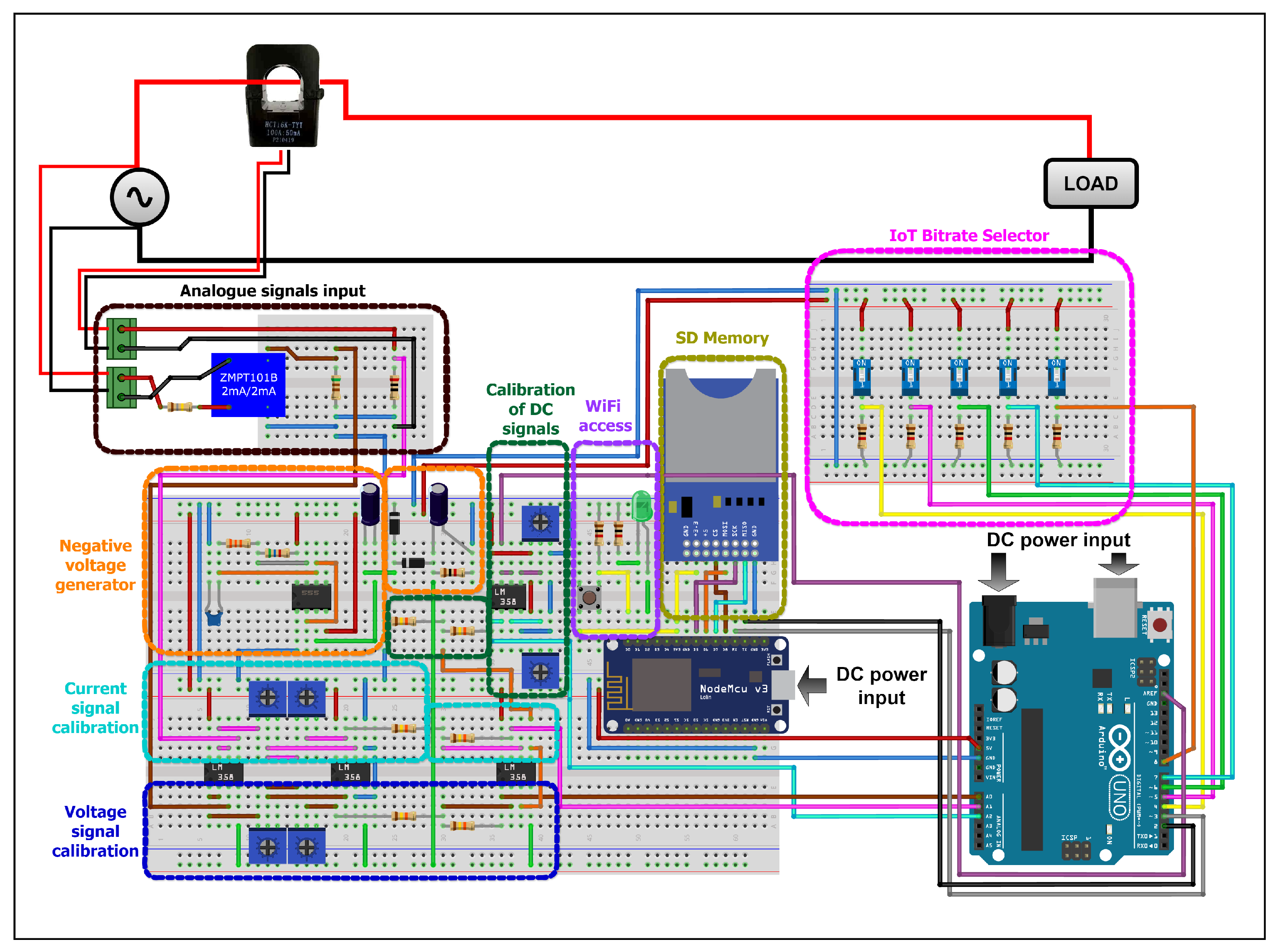
3.2. Hardware Detail Design

This section describes the design of the EPS hardware and the electronic components used, such as resistors, MCUs, and sensors, among others. Regarding MCU memories, SRAM is the memory where local variables are stored. Variables are created and manipulated during the MCU execution and supervised due to limited resource availability. The EEPROM is the physical memory where the data is stored after a reset or shutdown, featured by its electrical reprogramming capabilities.

On the other hand, the Arduino UNO (MCU ATmega328P) is the most suitable development board for this work, mainly because of its low cost and small physical dimensions. Also, the development board meets the characteristics of Flash memory, SRAM, EEPROM, analog inputs, and digital pins of this project, having a 32 kB Flash memory, a 2 kB SRAM memory, a 1 kB EEPROM memory, and a total of 6 analog inputs. In addition, the Arduino UNO has a write speed of 30 ms/B and a read speed of 0.4 us/B, mainly due to using the EEPROM. The Arduino UNO with MCU ATmega328P is valuable for low-cost prototyping but lacks industrial robustness and processing capabilities. For real applications featured by harsh environments (e.g., electromagnetic interference, high temperature, humidity, dust, and vibrations), industrial microcontrollers (e.g., STM32) with secure communication and EMI protection are recommended [45].

As for the hardware design of the EPS, the LM358 and NE555 integrated circuits were used to add the operational amplifiers, where the LM358 was used for the manual analog signal calibration functionality and the NE555 for the negative voltage generator. In addition, the noninvasive current sensors ZMPT101B (1:1 ratio) and HCT16K-TYT (1:2000 ratio) were used, where the former is used to measure the voltage and the latter the current. All the components used in the hardware design are low-cost and were already tested in the works mentioned in Section 2.1.

Figure 3 shows the general hardware schematic of the designed EPS. The schematic is in its Alpha (prototype) format. It shows parts such as voltage and current signal calibrations, DC signal calibration, IoT message rate selector, analog signal inputs, WiFi access, SD memory, and the used MCUs.

3.2.1. Variable Determination

Here, we present the mathematical models used in designing the EPS sensor suitable for EMS operation. It should be noted that the mathematical models are based on the design of the EPS and the use of an Arduino development board. Also, for calculating the electrical variables, the IEEE 1459-2010 standard [46] was used to a large extent. This standard is recommended for electrical energy measurements in sinusoidal, non-sinusoidal, balanced, or unbalanced conditions.

Figure 4 presents the schematic of the designed EPS, inspired by the work mentioned in Section 2.1. The sensor in question uses two noninvasive current sensors for the electrical system (AC voltage sensor and AC sensor), operational amplifiers with a negative voltage generator (based on NE555), and a DC voltage. As the signals delivered by the current and voltage sensors have negative values, a DC reference voltage is added to obtain only positive signals, as the Arduino development boards only read positive analog values (from 0 V to 3.3 V or 5 V, depending on the development board). In addition, the sensor has an analog reference output to be used on the AREF pin of the MCUs.

Continuing with the EPS design,

Table 4. Resistance values in the EPS hardware.

Resistance	Value at k$\mathbf{\Omega }$
$R_L$	180
$R_v$	0.51
$R_i$	0.02
$R_1$	5
$R_2$	5.042
$R_3$	5
$R_4$	10
$R_f$	14
$R_{AREF}$	4
$R_{ARE{F}_{Max}}$	10
$R_{DC}$	2
$R_{D{C}_{Max}}$	10

presents the resistance values shown in Figure 4.

The sensor in Figure 4 has two inputs ($V_{v_{in}}$ and $V_{i_{in}}$) and four outputs ($V_{v_{out}}$, $V_{i_{out}}$, $V_{D{C}_{ref}}$, and $V_{AREF}$). The first analog output $V_{v_{out}}$ represents the AC voltage sensor signal, where the input signal $V_{v_{in}}$ first passes through the separate operational amplifier $A_1$, then through the inverting operational amplifier $A_2$ to modify the amplitude of the signals using the variable resistors $R_1$ and $R_2$, and finally passes through the subtracting amplifier $A_3$, thus adding the reference $V_{D{C}_{ref}}$ to the signal. $V_{v_{out}}$ is defined in Equation (1).

$$V_{v_{out}}={\displaystyle \frac{R_2}{R_1}}{V}_{v_{in}}+{\displaystyle \frac{R_{DC}}{R_{D{C}_{MAX}}}}{V}_{DC}$$

(1)

The second analog output $V_{i_{out}}$ represents the load current signal, which has the same structure as the first analog output, with $A_4$ as the divider amplifier, $A_5$ as the inverting amplifier (with $R_3$ and $R_4$ as variable resistors), $A_6$ as the subtracting amplifier, and $V_{i_{in}}$ as an input signal. $V_{i_{out}}$ is presented in Equation (2).

$$V_{i_{out}}={\displaystyle \frac{R_4}{R_3}}{V}_{i_{in}}+{\displaystyle \frac{R_{DC}}{R_{D{C}_{MAX}}}}{V}_{DC}$$

(2)

The third analog output represents the reference signal $V_{D{C}_{ref}}$, which is obtained by the isolation amplifier $A_8$, where the input signal $V_{DC}$ is modified by the three-pin potentiometer $R_{DC}$, thus obtaining a variable resistance at the positive input of the amplifier. $V_{D{C}_{ref}}$ is given in Equation (3).

$$V_{D{C}_{ref}}={\displaystyle \frac{R_{DC}}{R_{D{C}_{MAX}}}}{V}_{DC}$$

(3)

Finally, the fourth $V_{AREF}$ output is an analog reference option that can be used on the AREF pin of the Arduino, whose output is represented in Equation (4) and uses the $A_7$ operational separator amplifier, modified by the $V_{DC}$ input voltage via the $R_{AREF}$ potentiometer.

$$V_{AREF}={\displaystyle \frac{R_{AREF}}{R_{ARE{F}_{MAX}}}}{V}_{DC}$$

(4)

One tool used in the calculations is the use of a Digital Low Pass Filter (Moving Average Filter) to remove the noise in $V_{D{C}_{ref}}$. The filter is shown in Equation (5) and has a smoothing factor D = 0.1 to obtain an acceptable attenuation.

$$V_{D{C}_{MM}}\left[k\right]=V_{D{C}_{ref}}\left[k\right]\ast 0.1+V_{D{C}_{MM}}[k-1]\ast 0.9$$

(5)

To calculate the variables, it is necessary to use Equations (6) and (7), where $k_v$ and $k_i$ are constants that depend on the relative accuracy of the Arduino and the resolution of the sensors.

$$V\left[k\right]=K_v(V_{v_{out}}\left[k\right]-V_{D{C}_{MM}}\left[k\right])$$

(6)

$$I\left[k\right]=K_v(V_{i_{out}}\left[k\right]-V_{D{C}_{MM}}\left[k\right])$$

(7)

Therefore, the determination of the variables $V_{RMS}$, $V_1$, $V_3$, $V_{THD}$, $I_{RMS}$, $I_1$, $I_3$, $I_{THD}$, S, P, Q, and FP is done using the following equations. Equation (8) shows the method for calculating the household electrical system’s $V_{RMS}$ value.

$$V_{RMS}=\sum _{k=1}^N\sqrt{{\displaystyle \frac{V{\left[k\right]}^2}{N}}}$$

(8)

The calculation of the fundamental voltage value is achieved using the Fourier series, where Equations (9) and (10) represent the Fourier coefficients, Equation (12) is the voltage phase angle, and Equation (11) is the $V_1$.

$$V_{a_1}={\displaystyle \frac{2(\mathsf{\Delta }T)}{T_o}}\sum _{k=1}^{N}V\left[k\right]cos[\omega [k-1]\mathsf{\Delta }T]$$

(9)

$$V_{b_1}={\displaystyle \frac{2(\mathsf{\Delta }T)}{T_o}}\sum _{k=1}^{N}V\left[k\right]sin[\omega [k-1]\mathsf{\Delta }T]$$

(10)

$$V_1=\sqrt{{V_{a_1}}^2+{V_{b_1}}^2}$$

(11)

$${\mathsf{\Theta }}_V=ta{n}^{-1}\left[{\displaystyle \frac{V_{b_1}}{V_{a_1}}}\right]$$

(12)

The value of the third harmonic voltage is obtained using the Fourier series, using Equations (13) and (14) to calculate the Fourier coefficients and Equation (15) to obtain the value of the $V_3$.

$$V_{a_3}={\displaystyle \frac{2(\mathsf{\Delta }T)}{T_o}}\sum _{k=1}^{N}V\left[k\right]cos\left[3(\omega [k-1]\mathsf{\Delta }T)\right]$$

(13)

$$V_{b_3}={\displaystyle \frac{2(\mathsf{\Delta }T)}{T_o}}\sum _{k=1}^{N}V\left[k\right]sin\left[3(\omega [k-1]\mathsf{\Delta }T)\right]$$

(14)

$$V_3=\sqrt{{V_{a_3}}^2+{V_{b_3}}^2}$$

(15)

Finally, the $V_{THD}$ is calculated using Equation (16).

$$V_{THD}={\displaystyle \frac{\sqrt{{V_{RMS}}^2-{V_1}^2}}{V_1}}$$

(16)

As for the current values, Equation (17) presents the method for calculating the household load’s $I_{RMS}$ value.

$$I_{RMS}=\sum _{k=1}^N\sqrt{{\displaystyle \frac{I{\left[k\right]}^2}{N}}}$$

(17)

The calculation of the fundamental current is obtained using the Fourier series, where Equations (18) and (19) represent the Fourier coefficients, Equation (21) is the current phase angle, and Equation (20) is the $I_1$.

$$I_{a_1}={\displaystyle \frac{2(\mathsf{\Delta }T)}{T_o}}\sum _{k=1}^{N}I\left[k\right]cos[\omega [k-1]\mathsf{\Delta }T]$$

(18)

$$I_{b_1}={\displaystyle \frac{2(\mathsf{\Delta }T)}{T_o}}\sum _{k=1}^{N}I\left[k\right]sin[\omega [k-1]\mathsf{\Delta }T]$$

(19)

$$I_1=\sqrt{{I_{a_1}}^2+{I_{b_1}}^2}$$

(20)

$${\mathsf{\Theta }}_I=ta{n}^{-1}\left[{\displaystyle \frac{I_{b_1}}{I_{a_1}}}\right]$$

(21)

The value of the third harmonic of the load current is obtained through the Fourier series, using Equations (22) and (23) to calculate the Fourier coefficients and Equation (24) to obtain the value of the $I_3$.

$$I_{a_3}={\displaystyle \frac{2(\mathsf{\Delta }T)}{T_o}}\sum _{k=1}^{N}I\left[k\right]cos\left[3(\omega [k-1]\mathsf{\Delta }T)\right]$$

(22)

$$I_{b_3}={\displaystyle \frac{2(\mathsf{\Delta }T)}{T_o}}\sum _{k=1}^{N}I\left[k\right]sin\left[3(\omega [k-1]\mathsf{\Delta }T)\right]$$

(23)

$$I_1=\sqrt{{I_{a_3}}^2+{I_{b_3}}^2}$$

(24)

Finally, the $I_{THD}$ calculation is obtained through Equation (25).

$$I_{THD}={\displaystyle \frac{\sqrt{{I_{RMS}}^2-{I_1}^2}}{I_1}}$$

(25)

The electrical power values are obtained once the current and voltage values have been calculated, where Equation (26) represents the S, Equation (27) the P, and Equation (28) the Q. Furthermore, the calculation of reactive power is not affected by the harmonic content of the system, as the powers are trigonometrically related.

$$S=V_{RMS}\ast I_{RMS}$$

(26)

$$P=\sum _{k=1}^N{\displaystyle \frac{V\left[k\right]\ast I\left[k\right]}{N}}$$

(27)

$$Q=\sqrt{S^2-P^2}$$

(28)

Finally, the FP is calculated by Equation (29). Also, referring to Equation (21), if ${\mathsf{\Theta }}_I$ is greater than or equal to zero, the load is inductive; conversely, if ${\mathsf{\Theta }}_I$ is less than zero, the load is capacitive.

$$FP={\displaystyle \frac{P}{S}}$$

(29)

3.2.2. Frequency Measurement

We propose a novel method of computing the value of the $F_e$ value. This method uses the second-order digital bandpass IIR filter (shown in Equation (30)) and the backward Euler approximation shown in Equation (31). Also, a measurement time of 20 ms was used for the operating $F_e$ of 50 Hz. The measurements may be affected if the system operates at other frequencies, as there could be a time lag that adds or subtracts values in the final measurements. A digital IIR filter was chosen because of its fast stability and low number of coefficients. In addition, phase information is not necessary for this application. For design, a center frequency of 50 Hz, a bandpass of 1.67 Hz (allows reading values from 49.165 to 50.835 Hz), and a sampling time of 200 us (measurement sampling time of the designed EPS). The bandpass value of 1.67 Hz was obtained based on a quality factor equal to 30. The bandpass value equals 30 times less than the nominal frequency value of 50 Hz, thus ensuring center frequency selectivity (49.8 to 50.2 Hz) and harmonic rejection.

Digital filter design parameters were obtained based on the Chilean Technical Standards, decreed by the National Energy Commission in the Technical Standard for Safety and Quality of Service, delivered in December 2019. Therefore, the regulation establishes that in Chile, the frequency of the electrical network must be between the range 49.8 to 50.2 Hz, with a 50 Hz central frequency of the digital filter [47].

$$\begin{array}{cc}\hfill V_{filter}\left[k\right]& =0.002091\left(V\right[k-1]-V[k-2\left]\right)\hfill \\ \hfill & +1.994V_{filter}[k-1]-0.9979V_{filter}[k-2]\hfill \end{array}$$

(30)

$$\omega Cos\left[\omega t\right]={\displaystyle \frac{Sin\left[\omega t\right]-Sin\left[\omega \right(t-\mathsf{\Delta }T\left)\right]}{\mathsf{\Delta }T}}$$

(31)

Figure 5 shows the $F_e$ calculation procedure. The method uses a digital filter and the backward Euler approximation.

The calculation process, shown in Figure 5, considers the following steps:

• Filter the voltage signal by simulating 2 s, using the digital filter of Equation (30). At this stage, the simulation time is essential because it is possible to obtain results quickly, for example, every 20 ms or one second.
• Calculate the RMS of the filtered signal; this is called the A-value.
• Derive by Equation (31) the filtered signal and obtain the RMS (this is called the B-value).
• Divide the B-value by A, then divide by $2\pi$.
• Obtain the frequency value.

3.2.3. Use of the Electrical Power Sensor Designed on a Microcontroller

Figure 6 represents the programming code flows of the MCUs. The Arduino UNO code uses 38%.

Figure 6a shows the diagram of the code used in the Arduino UNO. The code at startup enters the SETUP block, where the serial communication, analog reference, and digital inputs are initialized.

Then, on entering the BUCLE block, it first reads the DC reference using a Digital Low Pass Filter from Equation (5) for a time of 100 ms. Then, for a time of 20 ms (assuming a system frequency of 50 Hz), the measured voltage values are stored in a vector every 200 us, giving 100 data points. The same procedure is repeated to store the measured current signals. The variable calculation stage is performed in a period of 660 ms, using the procedures mentioned in Section 3.2.1, where the number of data is N = 100, the time of a period of a sine wave is $T_o$ = 20 ms, the angular velocity is $\omega$ = 100$\pi$ rad/s, and the sampling time is $\mathsf{\Delta }T$ = 200 $\mathsf{\mu }$s.

Finally, the calculated variables are sent to the serial ports, and the MCU work is paused (which takes 200 ms). Once the stages are finished, the LOOP block is started again, repeating the process (from DC reference reading to data sending) every 1 s. In the data-sending stage, the IoT data transmission time is selected, which is the time to send data from the Arduino UNO to the NodeMCU. The selection is done through a 5-pin switch module; the conditions are presented below:

• (No selection): 5 s.
• (Switch one only): 10 s.
• (Switch two only): 15 s.
• (Switch three only): 20 s.
• (Switch four only): 25 s.
• (Switch five only): 30 s.
• (more than one switch): The highest time is prioritized.

Figure 6b presents the coding scheme of the NodeMCU. First, the code is initialized, and then the START block is executed, where Internet connection functions, sending data to MQTT, serial port, and SD card connection are enabled. When entering the BUCLE block, if data is enabled in the serial communication, the received values are first assigned, saved on the SD card, and then sent to a port with MQTT communication. Then, the values are reset, the process pauses at 100 ms, and the user waits to receive new data. In addition, the program allows WiFi connection to any available network based on the procedure detailed below:

• Press the button for 5 s.
• The green LED lights up, indicating you are not connected to WiFi.
• Access the access point called “Electric-Meter.”
• Access an available WiFi network.
• Wait until the LED turns off (signal that you are now connected to the Internet).

Finally, the NodeMCU is not connected to WiFi if the LED flashes.

3.3. Software Detail Design

In this section, we present the designed SEM monitoring system. First, we selected the ARM Cortex-A72 MPU of the Raspberry PI 4 Model B development board to use the developed software.

The Raspberry Pi 4 CPU was chosen because of its affordable cost, 8 GB RAM capacity, 4 K video capability, 64-bit operating system, and low power consumption (maximum 15 W). The CPU can also run Node-RED, Arduino IDE, and MariaDB software tools.

In addition, the Raspberry Pi 4 Model B has a high memory read/write access speed due to its high CPU operating frequency (1.5 GHz), high RAM capacity, and large cache memories. The cache memory’s L1 memory has 32 kB of data and 48 kB of instruction, and the L2 memory has 1 MB.

The Node-RED flows designed to create the SEM measurement software are presented. These flows deliver functionalities such as an SQL database, a dashboard, and the use of an SS Sonoff. The software created in Node-RED is a JSON source file.

Figure 7 shows the Node-RED flow called “Input dates” with a file size of 1 kB; this flow receives data messages through SC and MQTT (JSON format messages), giving the option to select the type of communication, modify the message rate, and use an SS.

Figure 8 shows the Node-RED flow called “Serial dates” with a file size of 35 kB; the flow receives the message in JSON format, traces the variables in the control panel, calculates the energy consumed per minute, and stores the variables in a SQL database.

The Node-RED stream shown in Figure 9 is called ‘CPU status’, with a file size of 25 kB, it traces the Raspberry Pi CPU status variables, stores the values in a SQL database, and provides the option to shut down or reboot the device.

3.3.1. Interface

Figure 10 below shows the designed SEM control panel divided into three parts. Figure 10a shows the “Electric meter” control panel where the voltage, current, and power values are displayed, as well as a CPS with SS and voltage and frequency anomaly alerts. Figure 10b shows the “CPU status” control panel, which provides information about the CPU, RAM, and hard disk of the MPU, as well as the rate of messages received per minute and the option to change the type of communication. Finally, Figure 10c shows the “Exit” control panel, giving the user the alternative to shut down or reset the MPU.

The alarm system created in the control panel establishes an acceptable frequency between 49.8 and 50.2 Hz, based on the Chilean Technical Standards [47]. About voltage levels, an alarm system was decreed in the range of 220 to 240 V due to the specifications of the existing appliances in the SH. If the voltage is slightly below 220 V, the appliances will continue operating normally, although outside their nominal range.

We decided to create the alarm system in the 220 to 240 V range because appliances in this range operate at their nominal point, thus achieving better energy efficiency and a longer lifetime.

3.3.2. Using the Monitoring System Software Designed on a Microprocessor

Figure 11a shows the working structure of the measured variables. In the structure, the data is obtained by SC and MQTT, giving the option to select the type of communication. Then, a JSON object is created to display the variables in a dashboard, calculate the energy consumed per minute, store the measured variables in an SQL table, and give the option to use an SS Sonoff.

Figure 11b presents the architecture to evaluate the state of the Raspberry Pi 4. It can be seen that the data is updated every 10 s through a LOOP, delivering values such as CPU usage percentage, RAM usage percentage, hard disk usage percentage, CPU temperature in °C, and message-sending rate per minute. Once the data is read, it is stored in an SQL database (data is saved every 1 min) and can be displayed on a control panel. Furthermore, the importance of visualizing and keeping this data lies mainly in the study and Monitoring of the CPU performance, as this way, problems can be identified, failures can be avoided, and/or decision-making on the computer can be improved. Figure 11a shows the working structure of the measured variables. In the structure, the data is obtained by SC and MQTT, giving the option to select the type of communication. Then, a JSON object is created to display the variables in a dashboard, calculate the energy consumed per minute, store the measured variables in an SQL table, and give the option to use an SS Sonoff.

Figure 11b presents the architecture to evaluate the state of the Raspberry Pi 4. It can be seen that the data is updated every 10 s through an LOOP, delivering values such as CPU usage percentage, RAM usage percentage, hard disk usage percentage, CPU temperature in °C, and message-sending rate per minute. Once the data is read, it is stored in an SQL database (data is saved every 1 min) and can be displayed on a control panel. Furthermore, the importance of visualizing and keeping this data lies mainly in the study and monitoring of the CPU performance, as this way, problems can be identified, failures can be avoided, and/or decision-making on the computer can be improved.

The control panel allows us to access the Raspberry Pi 4 status data, select the type of communication (MQTT or SC), and restart or shut down the CPU. The CPU restart and shutdown functionalities can also be used as an emergency system in case the user detects anomalies in the computer’s operation. In addition, the novel method of selecting the type of communication allows the user to have great flexibility in displaying data.

4. SEM Evaluation

In the following section, a series of measurement tests are presented to evaluate the performance of the designed SEM. Specifically, we study the behavior of the EPS hardware and the monitoring system software. Figure 12 shows the SEM created by measuring the household consumption. It should be noted that the SEM is in the prototyping phase (Alpha stage).

4.1. Numerical Experiments

Numerical experiments were carried out using PSIM software to corroborate the methods and equations shown in this chapter. During the evaluation, measurements were performed on a single-phase electrical system, simulating using an MCU as an SEM. In addition, the system fed a resistive, inductive, and capacitive load.

During the experiments, the CPU used is an HP Pavilion Laptop 15-cs3, with an Intel(R) Core(TM) i7-1065G7 CPU @ 1.30 GHz and 12 GB RAM. The test was performed on a PSIM file of size 52 kB. The simulation time was 1 s, and the results on the computer were obtained in 1 min and 2 s.

The values of the power grid were measured, where the voltage was simulated from Equation (32), at a $F_e$ of 50 Hz. Test voltage has harmonic content ranging from the fundamental value to the 49th harmonic.

$$V_{test}=\sum _{k=2i-1}^{49}{\displaystyle \frac{220\sqrt{2}}{k}}sin\left[k\left(\omega t\right)\right]\Rightarrow with:1\le i\le 25$$

(32)

Table 5. Numerical experiment on power grid variables.

Variable	Real Value	Measured Value	Error %
$V_{RMS}$	243.354	243.362	0.003
$V_1$	220	219.988	−0.005
$V_3$	73.333	73.330	−0.005
$V_{THD}$	46.929	47.316	0.825
$F_e$	50	49.999	−0.002

presents the results of the percentage error for the measurements of the main variables, such as voltages and frequency values. On this basis, the calculated percentage of error for all variables is less than 1%, which shows that the calculation methods are accurate when used on an MCU with a sampling time of 20 ms.

The values related to the loads, the currents, and the power were then measured. In the simulation, from the start until 0.4 s, a 20 $\mathsf{\Omega }$ resistor was connected, thus simulating a resistive load. Then, from 0.4 to 0.6 s, a 10 $\mathsf{\Omega }$ resistor and a 10 mH inductance were operated, therefore obtaining an inductive load. At the end of the simulation, from 0.6 to 1 s, a 10 $\mathsf{\Omega }$ resistor and a 500 uF capacitor were operated, thus evaluating a capacitive load. The following tables show the simulation results of the measured load variables, such as currents and powers, where

Table 6. Numerical experimentation of load measurements: resistive load.

Variable	Real Value	Measured Value	Error
$I_{RMS}$	12.169	12.169	0.000
$I_1$	11.001	11.001	0.000
$I_3$	3.667	3.667	0.000
$I_{THD}$	46.929	47.297	0.784
P	2961.387	2961.333	−0.002
Q	0.000	0.000	0.000
S	2961.375	2961.333	−0.002
$FP$	1.000	1.000	0.000

represents the resistive load,

Table 7. Numerical experimentation of load measurements: inductive load.

Variable	Real Value	Measured Value	Error
$I_{RMS}$	21.858	21.856	−0.009
$I_1$	20.989	20.989	0.000
$I_3$	5.337	5.337	0.000
$I_{THD}$	28.762	29.053	1.012
P	4776.773	4777.778	0.021
Q	2340.228	2337.247	−0.127
S	5319.232	5318.824	0.008
$FP$	0.898	0.898	0.000

the inductive load and

Table 8. Numerical experimentation of load measurements: capacitive load.

Variable	Real Value	Measured Value	Error
$I_{RMS}$	21.212	21.208	−0.019
$I_1$	18.560	18.556	−0.022
$I_3$	7.174	7.173	−0.014
$I_{THD}$	54.894	55.362	0.853
P	4499.035	4499.293	0.006
Q	2530.847	2530.132	−0.028
S	5162.025	5161.899	−0.002
$FP$	−0.872	−0.872	0.000

the capacitive load.

The results indicate that the proposed measurement methods are effective, achieving relative errors below 1.02%, with the highest relative errors associated with THD. Additionally, the largest relative error calculated was for the $I_{THD}$ of the inductive load. The accuracy of SEM is affected when monitoring nonlinear loads, such as phase-controlled rectifiers and diode rectifiers, which introduce significant harmonic distortion into the electrical system. Despite the SEM’s advanced measurement capabilities, certain parameters show slight variations in accuracy under these conditions. For voltage and current RMS measurements (VRMS, IRMS), the SEM employs noninvasive sensors (ZMPT101B and HCT16K-TYT), providing a relative error of less than 0.5% under standard conditions. However, as presented in Table 5 (Numerical Experiment on Power Grid Variables), the VRMS measurement error slightly increases for waveforms with high harmonic content, reaching up to 0.82% in VTHD calculations. This indicates that while the SEM maintains high accuracy, distorted waveforms from nonlinear loads may introduce minor deviations in RMS values. Regarding harmonic analysis and Total Harmonic Distortion (THD), the SEM uses a Fourier Transform-based method to extract harmonic components from the measured signals. Under nonlinear conditions, higher-order harmonics (e.g., 3rd, 5th, and 7th harmonics) influence the THD computation.

Table 7 (Inductive Load) and Table 8 (Capacitive Load) demonstrate that the ITHD measurement error reaches 1.02%, particularly when the system operates with high harmonic content. Although this signifies a slight increase in uncertainty, the SEM remains highly accurate for harmonic monitoring. For active (P) and reactive power (Q) calculations, the SEM adheres to the IEEE 1459-2010 standard, ensuring robustness against waveform distortion. The experimental numerical results in Table 6 (Resistive Load), Table 7 (Inductive Load), and Table 8 (Capacitive Load) show that P and Q measurement errors stay below 0.15%, even under nonlinear load conditions. This emphasizes the SEM’s effective precision in power measurements despite distorted waveforms. While the SEM offers reliable measurements for nonlinear loads, minor deviations occur in VRMS, IRMS, and THD values, particularly under high harmonic conditions. These findings indicate that additional sensor calibration or adaptive signal processing techniques could enhance measurement accuracy in industrial applications involving nonlinear power electronics loads.

4.2. Uncertainty Analysis of Measurements

To evaluate the calibration performance of the EPS on the designed SEM, measurements were taken over approximately 13 h, saving data every 10 s and collecting a total of 4916 samples. Also, the values measured by the MI 2883 Energy Master, using the modern method (IEEE 1459 [46]), were considered as real or standard values. In addition, measurements were evaluated in different regions of operation concerning apparent power. For the low consumption area, loads equal to or less than 300 VA were considered; for medium consumption loads above 300 VA and less than or equal to 1000 VA; and high consumption loads above 1000 VA. Concerning the limitations of SEM, they can be presented when operating in extreme environmental conditions. High temperatures beyond its operational range (0 °C to 85 °C) may degrade performance or cause hardware failures. Humidity and dust exposure can lead to corrosion and short circuits due to the lack of protective coatings. Additionally, electromagnetic interference (EMI) from industrial equipment may introduce noise in measurements, decreasing the accuracy, and fluctuations in the input voltage may cause failures due to the absence of overvoltage protection.

4.2.1. Measurement Tests

Results of measurements performed by the ESP and their analysis are presented. First, Figure 13 shows the measurements obtained from the electrical system used to power the SH.

The designed EPS provides accurate measurement of the electric variables, where part (a) represents the $V_{RMS}$, part (b) the $V_1$, part (c) the $V_3$, part (d) the $V_{THD}$, and part (e) the system $F_e$. Of note, there is a low harmonic content in the voltage (less than 9%), an $V_{RMS}$ within the range of 215 to 235 V, and a system $F_e$ operating between 49.5 to 50.5 Hz.

The current measurements are shown in Figure 14, where the EPS provides accurate measurements considered as a benchmark. Part (a) shows the $I_{RMS}$, part (b) the $I_1$, part (c) the $I_3$, and part (d) the $I_{THD}$. It is observed that the $I_{RMS}$ ranges from 0 to 12 A. Furthermore, the load current of the SH has a significant harmonic content, oscillating at an average $I_{THD}$ of 40% (reaching values up to 120%), resulting in a $I_3$ of values up to 1 A.

Figure 15 shows the power consumption ((a) P, (b) Q, (c) S, and (d) FP, respectively), highlighting that the designed EPS provides accurate power and energy measurements concerning its benchmark values.

Figure 16 shows the linear regressions comparing the power values measured by the EPS (P, Q, and S) with those tested by the benchmark meter. Here, 2586 low-power tests, 2151 medium-power measurements, and 238 high-power measurements were analyzed. Figure 16a P, Figure 16b Q, and Figure 16c S, respectively.

Equation (33) represents the highly accurate linear regression of the P calibration. The equation boasts an $R^2$ equal to 0.999, indicating a near-perfect distribution of the data, with the model able to reference almost all the data points. Equation (34) demonstrates the precise linear regression of the Q calibration of the designed EPS. The equation has an $R^2$ equal to 0.9549, showing that the linear regression explains the variability of the data well, referencing around 95%.

$$\widehat{Y}\left[\widehat{X}\right]\approx 0.9996\ast \widehat{X}-0.1605$$

(33)

$$\widehat{Y}\left[\widehat{X}\right]\approx 0.9901\ast \widehat{X}-1.0933$$

(34)

$$\widehat{Y}\left[\widehat{X}\right]\approx 0.9995\ast \widehat{X}-0.1255$$

(35)

From the above, it is demonstrated that the designed EPS provides an accurate measurement of the consumption profile by means of P, Q, and S, independently of the apparent power consumption operation zone.

4.2.2. Accuracy Testing

Table 9. Error analysis of the designed EPS: relative errors.

Variable	${\mathit{e}}_{{\mathit{a}}_{\mathit{Maximum}}}$	${\mathit{e}}_{{\mathit{a}}_{\mathit{Minimum}}}$	${\mathit{E}}_{{\mathit{a}}_{\mathit{Maximum}}}$	${\mathit{E}}_{{\mathit{a}}_{\mathit{Minimum}}}$
$V_{RMS}$	6.710	0.000	2.954	0.000
$V_1$	6.681	0.000	2.947	0.000
$V_3$	1.086	0.000	19.996	0.000
$V_{THD}$	1.858	0.000	29.142	0.000
$I_{RMS}$	0.477	0.000	10.000	0.000
$I_1$	0.467	0.000	17.108	0.000
$I_3$	0.192	0.000	20.000	0.000
$I_{THD}$	24.789	0.000	29.973	0.000
P	109.937	0.002	22.053	0.001
Q	73.348	0.001	24.917	0.001
S	112.021	0.002	10.410	0.001
$FP$	0.107	0.000	14.996	0.000
$F_e$	0.255	0.000	0.508	0.000

and

Table 10. Error analysis of the designed EPS: error metrics.

Variable	MRE	MAPE	RMSE	${\mathit{s}}^2$	${\mathit{e}}_{\mathit{R}}$	${\mathit{R}}^2$
$V_{RMS}$	−0.004	0.231	0.711	0.711	0.020	0.948
$V_1$	−0.004	0.230	0.710	0.710	0.020	0.948
$V_3$	−0.166	6.603	0.288	0.288	0.008	0.921
$V_{THD}$	0.060	3.039	0.279	0.279	0.008	0.149
$I_{RMS}$	−0.052	2.794	0.054	0.054	0.002	0.999
$I_1$	−0.076	2.781	0.050	0.050	0.001	0.999
$I_3$	−0.196	5.440	0.033	0.033	0.001	0.977
$I_{THD}$	0.049	7.544	5.231	5.232	0.145	0.919
P	−0.084	3.105	11.810	11.808	0.328	0.999
Q	−0.142	5.676	11.336	11.331	0.315	0.955
S	−0.056	2.815	12.475	12.473	0.347	0.999
$FP$	−0.017	1.676	0.018	0.018	0.001	0.978
$F_e$	−0.101	0.153	0.092	0.077	0.002	0.001

show the key performance indices calculated for the accuracy testing of SEM to quantify its accuracy, according to the index defined in Appendix A. Table 9 represents the relative errors, and Table 10 represents the absolute error metrics. The results show that the MAPEs and MREs present low values, demonstrating the accuracy of the measurements performed by SEM. In addition, the values of MREs vary between 0 to 0.2%, and the MAPEs do not exceed the value of 7%.

Accuracy testing of P, Q, and S presents a low value of the error-based performance indices, being the lowest the power S with an RMSE of 12.475 VA, an $s^2$ of 12.473 VA, and an $e_R$ of 0.347 VA. From the above, it can be verified a high accuracy by SEM. Correlation coefficient $R^2$ reports satisfactory results, with values mostly over 0.94. Regarding $V_{THD}$ and $F_e$, which exhibit $R^2$ values of 0.149 and 0.001, respectively, those values could be related to the stability of the measurements that can be ruled out, since $V_{THD}$ remains at around 6% and $F_e$ at 50 Hz. Furthermore, in the case of $F_e$ (frequency), the values did not change significantly due to the need to use lower sampling times. It is essential to note that the EPS can be affected by significant measurement errors, which can be attributed to several factors, such as MCU performance, NICS accuracy, tolerance of the resistors used (between 5% and 10%), and exposure to humidity and ambient temperature fluctuations.

Next, box plot diagrams are shown by the EPS, carrying out studies with the totality of the data obtained and with the respective apparent power operation zones. Figure 17 shows the box plots of the variables delivered by the SH electrical system. Part (a) represents the $V_{RMS}$, part (b) the $V_1$, part (c) the $V_3$, part (d) the $V_{THD}$ (e), and part $F_e$. Generally, the apparent power consumption zones do not alter the measurement errors. Figure 18 shows the box plots of the current variables, where (a) deploys the $I_{RMS}$, (b) deploys $I_1$, (c) deploys $I_3$, and (d) deploys $I_{THD}$. From the results in Figure 18, it is observed that the calculated error of the current increases in proportion to the apparent power consumption. Therefore, the highest error values are presented in an operation with high power. Also, $I_{THD}$ decreases as the current increases, proving that the harmonic content is higher at low consumption currents.

Figure 19 shows the box plots of the measured powers, where Figure 19a deploys P, Figure 19b deploys Q, Figure 19c deploys S, and Figure 19d deploys FP. From these results, it is verified that the error of the calculated power increases with the apparent power consumption, proving that the zone of high power consumption has the highest calculated error. In addition, in the high power consumption area, the power factor presents few variations, proving that the high consumption loads of the SH tend to be more of the resistive type.

The box plot diagrams show that the measurements across all the operation zones present an average value close to 0. Furthermore, it is apparent that, at high powers, the measurement error of the variables associated with EPS current and power amplifies, presenting larger interquartile ranges in the high consumption zone. In practical terms, the higher the consumption, the more likely the measured power error will increase, which has significant implications for power system management.

4.3. Computational Performance

A study of the CPU’s behavior as a function of the rate of messages sent per minute was carried out using the software created in Node-RED. During the experiment, tests were performed with different message rates varying from 1 to 10 s. The experiment evaluated how the MPU behaves at various operating points, thus finding the optimal operating point and corroborating the worst-case performance. The tests were carried out in 1 h and 40 min, varying the frequency of the messages every 10 min. In this case, we proceeded to analyze the results by obtaining the mean and variances of the data.

Table 11. Analysis of results of CPU variables.

Variable	% CPU Usage		CPU Temperature in °C		% RAM Usage		% Disk Usage		Massage Rate Per Minute
Massage Delay in Seconds	$\overline{\mathit{X}}$	${\mathit{s}}^{\mathbf{2}}$	$\overline{\mathit{X}}$	${\mathit{s}}^{\mathbf{2}}$	$\overline{\mathit{X}}$	${\mathit{s}}^{\mathbf{2}}$	$\overline{\mathit{X}}$	${\mathit{s}}^{\mathbf{2}}$	$\overline{\mathit{X}}$	${\mathit{s}}^{\mathbf{2}}$
1	9.0500	3.6096	30.693	1.2813	12.43	0.0122	27	0	39.183	12.5251
2	9.171	1.6591	30.947	0.4608	12.633	0.0029	27	0	25.634	9.4354
3	8.917	2.6985	30.862	0.7516	12.627	0.0027	27	0	18.61	0.7592
4	8.378	2.0428	30.717	0.7464	12.652	0.0029	27	0	14.322	0.5324
5	8.263	3.0061	30.500	0.3240	12.810	0.0029	27	0	11.627	0.2379
6	9.238	11.836	30.996	0.5764	12.964	0.0037	27	0	9.85	0.1297
7	8.775	2.1244	31.049	0.4366	13.138	0.0108	27	0	8.407	0.2455
8	8.554	2.7110	31.279	0.3335	13.154	0.0097	27	0	7.407	0.2455
9	8.694	2.6073	31.079	0.3438	13.137	0.0036	27	0	6.593	0.2455
10	9.837	29.173	31.111	0.8497	13.428	0.0198	27	0	6.0000	0.0000

reports the response of the CPU in terms of percentage of usage rate and temperature, showing that the mean CPU usage and temperature do not vary significantly with changes in the message rate. Also, the variance value remains independent from the message rate, but in the case of messages with a 6 and 10 s delay, the variance is high because the CPU usage increases drastically, which could be explained by the presence of multiple software threads using the same hardware resources.

In addition, other elements analyzed are shown, such as the results obtained for RAM portability, hard disk, and message per minute rate. The study shows that mean and variance values do not change drastically with changes in message rates. Furthermore, the variance of hard disk usage is zero, and the variance of RAM usage is almost zero. Another result to note is the increased RAM usage with a slight increase in message rates. The study of the message-sending rate reveals that the behavior is optimal from when a message is sent every 4 s, reaching the desired value when messages are sent every 10 s, reaching a variance equal to zero. Finally, Figure 20 shows the data presented in Table 11. The figure is composed of four parts: (a), (b), (c), and (d). Part (a) shows the CPU usage percentage data, part (b) presents the CPU temperature, part (c) shows the RAM usage percentage, and part (d) shows the message per minute rate. The best operation point is when the message delay is 10 s because the message rate does not show variations, and the other physical variables of CPU and RAM have adequate behavior as expected.

Assessment of Communications Performance

In the following, we delve into the characteristics and properties of the communication from the EPS (sender) to the CPU (receiver). In general terms, the most secure and efficient communication is SC. It delivers a higher data rate, is less susceptible to interference, and provides robust security against remote attacks. Moreover, ESP is designed as a stationary (non-mobile) device, making the SC path suitable. However, it is important to note that SC lacks authentication methods, which could be a potential security concern. In such cases, we recommend using MQTT communication over SC, mainly when the EPS is located in a difficult-to-access and/or narrow place, making it impossible to physically connect the sensor to the CPU and/or any monitor. This mode of communication offers robust authentication methods, ensuring data security. In Figure 21, which is sectioned into parts (a), (b), (c), and (d), the behavior of the physical variables of the CPU can be visualized, where variables were tested every one minute, saving a total of 3480 data (2 days and 10 h). The experiment started using the SC, the best-evaluated case, using a rate of 60 messages per minute, which the MPU software delays to 6 messages per minute. Then, in data N°1930 (1 day, 8 h, and 10 min), MQTT communication via WiFi (sender and receiver with WiFi technology) was used, which is the worst case evaluated, varying the rate of messages per minute in values such as 12, 6, 4, 3, 2.4, and 2. Part (a) of the figure, which represents the percentage of CPU usage, shows that when the SC path is used, the average of the displayed data is 6.19%. In contrast, in MQTT communication, the average percentage of CPU usage increases to 8.77%. When using MQTT communication via WiFi instead of SC, the CPU system performance tends to be a bit slower, which hinders the execution of parallel tasks. Part (b) of the figure, representing the CPU temperature, shows no significant variations when changing the communication method. From part (c), it is observed that the percentage of RAM usage is an average of 11.91% when using the SC. When using the MQTT path with the WiFi network without interference, the average RAM usage increases to 12.89%. On the other hand, when MQTT communication is performed and the WiFi network suffers interference, the RAM usage drops to 12.7%, but the value is still higher than that shown when working with SC. From part (d) of the figure where the message rate per minute is observed, it can be evidenced that when the SEM uses the SC, the message rate varies between 5 and 6 per minute. Then, when using the MQTT communication, the message rate changes, delivering an amount of 0 to 12 messages per minute, thus demonstrating that the EPS fulfills its functionality of varying the data rate.

Furthermore, when switching from SC to MQTT communication, it is observed that the message rate remains stable (delivery of 5 to 6 messages per minute), but after some time, the number of messages presents greater variations, showing at the end that the messages no longer reach the CPU (0 messages per minute). Thus, it is shown that the message rate is directly affected if the WiFi path suffers interference and/or instability.

In summary, the SEM CPU is generally forced to do more work when using MQTT communication technology. In addition, when interference occurs, the message rate is affected, causing problems with data transmission.

4.4. Limitations and Implications

Although some features of the designed SEM share similarities with existing solutions in the literature, the novelty lies in how these elements are integrated into a flexible system capable of adapting to different user and application requirements. The most significant contribution is the possibility of using any NICSs to measure the load current, enabled by the manual calibration system embedded in the designed EPS. Specifically, the following features distinguish our approach:

• Use current sensors that are not invasive to the electrical system.
• Manual signal calibration system.
• Alternative use with different MCUs, thanks to its alternative to regulate the analog references.
• Possibility to change the data sending rate via MQTT.
• Option to connect to any WiFi network.
• Choice of communication channel in the monitoring system, either SC or MQTT.
• Possibility of using an SS in household appliances with consumption less than or equal to 10 A.
• New method of measuring electrical frequency.

Although non-invasive current sensors, manual calibration procedures, and MQTT-based communication have been explored individually in previous work, our contribution unifies these techniques within a single and adaptable framework. This integrated design—combining manual calibration for various NICSs, multi-communication support, and an alternative method for frequency measurement—offers a distinctive approach for energy monitoring systems.

Our ongoing work is to move forward with the developed prototype from the laboratory stage to the market stage. However, there are many considerations and requirements that still need to be addressed before moving to such a step, examples as given below:

• Define the target market: In our work, we considered the installation of the smart energy meter at the end-user domain (consumer); however, other market domains are also available, with different requirements, such as industrial domain and utility-scale.
• Define the environmental conditions: In our work, the installation of the smart energy meter was done indoors at the end-user domain (consumer). Special consideration should be given if the installation will be done outdoors, considering the environmental conditions of temperature, dust, humidity, and electromagnetic interference.
• Certification and Regulation: In general, the smart meter must comply with different industry standards such as meter accuracy and quality management standards. This means that the regulation and certifications of the smart energy meter in the Chilean market should be considered.
• PCB Design: Considering that the first prototype was implemented and tested using a breadboard, there is a need to develop and implement the PCB of the SEM solution. Such a prototype needs to be tested under real-world conditions for a long-term period in order to improve the current design.
• Development of a mobile application: Existing technologies on mobile phone devices can enhance the efficiency of real-time energy monitoring. This can be done through the development of a mobile application that includes different features such as real-time energy usage, anomaly detection, cost estimation, and alerts for faults.
• End-to-end energy consumption of SEM: For IoT devices, the energy consumption depends on multiple factors, e.g., the type of sensor nodes (active/passive), the power supply, the operation mode (active/sleep), and the communication protocols. Based on the target application of SEM, the system can generate low/high data volume. Therefore, the analysis of the end-to-end energy consumption of SEM should be divided into three main parts: the IoT devices part, the networking part, and the cloud part.

5. Conclusions

The designed SEM complies with the assigned functions and capabilities that can be used in industrial systems and smart homes, contributing significantly to EMS and home energy management systems. The developed SEM supports Industry 4.0 and IoT technologies and implements CPSs and cybersecurity features to protect against unauthorized access to the measurements. Furthermore, SEM remains suitable for performing data analysis in situ. The developed solution implemented the MQTT protocol for the communication between the EPS and the data monitoring system software. The dashboard has an alarm system for $F_e$ and $V_{RMS}$ measurements. The SEM can use a smart switch, thus creating a CPS in the smart home. Also, the device measures the physical variables of the CPU, opening the possibility of performing SEM as a CPS, including physical and cybernetic variables for system monitoring.

Regarding data storage system, the SEM has an SQL database through the MariaDB tool, which allows data analysis and cybersecurity of the measurements. The SEM results reveal MAPEs of less than 7% for the $V_{RMS}$, $V_1$, and $V_3$ voltage variables. For the load current variables, the MAPEs of $I_{RMS}$, $I_1$, and $I_3$ reach values below 6%. As for the power variables, P and S present $R^2$ close to 1, although Q registers an $R^2$ value of 0.955. In addition, the MAPEs for THD vary between 3% and 7.6%. An encouraging fact stands out, as all values show a minimum $E_A$ close to 0%, thus demonstrating the measurement accuracy of the SEM. However, this accuracy can be affected by external factors such as environmental conditions and the quality of the electronic components.

To evaluate the monitoring system software, we studied the CPU’s physical components, highlighting the message rate. Firstly, it is verified that the SEM operates optimally if the message delay exceeds 4 s, obtaining the desired value when the message delay is 10 s. The designed device can be used in single-phase power systems, delivering measurements of variables such as $V_{RMS}$, $V_1$, $V_3$, $V_{THD}$, $I_{RMS}$, $I_1$, $I_3$, $I_{THD}$, S, P, Q, FP, and $F_e$. Also, it was possible to measure the physical variables of the CPU, such as CPU usage percentage, CPU temperature, RAM usage percentage, hard disk usage percentage, and message data rate per minute.

Future work for the designed SEM will be considered to improve the accuracy of the measurements, either by changing the Arduino UNO for an MCU with better processing or by modifying the methods of calculating variables. The novel frequency measurement method can also be an alternative for improvement, as an analog one can replace the digital filter to decrease the MCU’s computational load. The SQL database can also be an alternative for improvement by creating a system that separates measured data by days, weeks, months, and years. Finally, future works consider SEM as the core of energy management systems to reach sustainable development goals related to energy monitoring and optimization.

References

1. Sustainable Development Goals. 2015. Available online: https://www.un.org/sustainabledevelopment/es/objetivos-de-desarrollo-sostenible/ (accessed on 10 December 2024).
2. Energy Efficiency Law, Chile. 2021. Available online: https://energia.gob.cl/ley-y-plan-de-eficiencia-energetica (accessed on 10 December 2024).
3. Alotaibi, I.; Abido, M.A.; Khalid, M.; Savkin, A.V. A comprehensive review of recent advances in smart grids: A sustainable future with renewable energy resources. Energies 2020, 13, 6269. [Google Scholar] [CrossRef]
4. Yem Souhe, F.G.; Boum, A.T.; Ele, P.; Mbey, C.F.; Foba Kakeu, V.J. A novel smart method for state estimation in a smart grid using smart meter data. Appl. Comput. Intell. Soft Comput. 2022, 2022, 7978263. [Google Scholar] [CrossRef]
5. Mazhar, T.; Irfan, H.M.; Haq, I.; Ullah, I.; Ashraf, M.; Shloul, T.A.; Ghadi, Y.Y.; Imran; Elkamchouchi, D.H. Analysis of Challenges and Solutions of IoT in Smart Grids Using AI and Machine Learning Techniques: A Review. Electronics 2023, 12, 242. [Google Scholar] [CrossRef]
6. Chakraborty, S.; Das, S.; Sidhu, T.; Siva, A. Smart meters for enhancing protection and monitoring functions in emerging distribution systems. Int. J. Electr. Power Energy Syst. 2021, 127, 106626. [Google Scholar] [CrossRef]
7. Elma, O.; Kuzlu, M.; Zohrabi, N. Internet of energy for renewable energy-based decarbonized electrical energy systems. Front. Energy Res. 2023, 11, 1160184. [Google Scholar] [CrossRef]
8. Saleem, Y.; Crespi, N.; Rehmani, M.H.; Copeland, R. Internet of things-aided smart grid: Technologies, architectures, applications, prototypes, and future research directions. IEEE Access 2019, 7, 62962–63003. [Google Scholar] [CrossRef]
9. Bedi, G.; Venayagamoorthy, G.K.; Singh, R.; Brooks, R.R.; Wang, K.C. Review of Internet of Things (IoT) in electric power and energy systems. IEEE Internet Things J. 2018, 5, 847–870. [Google Scholar] [CrossRef]
10. Baidya, S.; Potdar, V.; Ray, P.P.; Nandi, C. Reviewing the opportunities, challenges, and future directions for the digitalization of energy. Energy Res. Soc. Sci. 2021, 81, 102243. [Google Scholar] [CrossRef]
11. Hoang, A.T.; Nguyen, X.P. Integrating renewable sources into energy system for smart city as a sagacious strategy towards clean and sustainable process. J. Clean. Prod. 2021, 305, 127161. [Google Scholar] [CrossRef]
12. Kua, J.; Hossain, M.B.; Natgunanathan, I.; Xiang, Y. Privacy Preservation in Smart Meters: Current Status, Challenges and Future Directions. Sensors 2023, 23, 3697. [Google Scholar] [CrossRef]
13. Sovacool, B.K.; Hook, A.; Sareen, S.; Geels, F.W. Global sustainability, innovation and governance dynamics of national smart electricity meter transitions. Glob. Environ. Change 2021, 68, 102272. [Google Scholar] [CrossRef]
14. Singh, S.; Selvan, M. A smart energy meter enabling self-demand response of consumers in smart cities of Tamil Nadu. In Proceedings of the 2019 IEEE International Conference on Smart Cities Model (ICSCM), Chennai, India, 20–21 January 2019; pp. 1–6. [Google Scholar]
15. Muralidhara, S.; Hegde, N.; Rekha, P. An internet of things-based smart energy meter for monitoring device-level consumption of energy. Comput. Electr. Eng. 2020, 87, 106772. [Google Scholar] [CrossRef]
16. Lin, T.R.; Khan, N.H.O.; Daud, M.Z. Arduino based Appliance Monitoring System using SCT-013 Current and ZMPT101B Voltage Sensors. Prz. Elektrotechniczny 2021, 97, 89. [Google Scholar] [CrossRef]
17. Patel, H.K.; Mody, T.; Goyal, A. Arduino based smart energy meter using GSM. In Proceedings of the 2019 4th International Conference on Internet of Things: Smart Innovation and Usages (IoT-SIU), Ghaziabad, India, 18–19 April 2019; pp. 1–6. [Google Scholar]
18. Mlakić, D.; Baghaee, H.R.; Nikolovski, S.; Vukobratović, M.; Balkić, Z. Conceptual design of iot-based amr systems based on iec 61850 microgrid communication configuration using open-source hardware/software ied. Energies 2019, 12, 4281. [Google Scholar] [CrossRef]
19. Sayed, S.; Hussain, T.; Gastli, A.; Benammar, M. Design and realization of an open-source and modular smart meter. Energy Sci. Eng. 2019, 7, 1405–1422. [Google Scholar] [CrossRef]
20. Kumar, L.A.; Indragandhi, V.; Selvamathi, R.; Vijayakumar, V.; Ravi, L.; Subramaniyaswamy, V. Design, power quality analysis, and implementation of smart energy meter using internet of things. Comput. Electr. Eng. 2021, 93, 107203. [Google Scholar] [CrossRef]
21. Rathee, S.; Goyal, A.; Shukla, A. Designing prepaid smart energy meter and deployment in a network. In Proceedings of the 2020 IEEE 4th Information Technology, Networking, Electronic and Automation Control Conference (ITNEC), Chongqing, China, 12–14 June 2020; Volume 1, pp. 1208–1211. [Google Scholar]
22. Sanchez-Sutil, F.; Cano-Ortega, A.; Hernandez, J.; Rus-Casas, C. Development and calibration of an open source, low-cost power smart meter prototype for PV household-prosumers. Electronics 2019, 8, 878. [Google Scholar] [CrossRef]
23. Faisal, M.; Karim, T.F.; Pavel, A.R.; Hossen, M.S.; Lipu, M.H. Development of smart energy meter for energy cost analysis of conventional grid and solar energy. In Proceedings of the 2019 International Conference on Robotics, Electrical and Signal Processing Techniques (ICREST), Dhaka, Bangladesh, 10–12 January 2019; pp. 91–95. [Google Scholar]
24. Das, N.C.; Zim, M.Z.H.; Sarkar, M.S. Electric Energy Meter System Integrated with Machine Learning and Conducted by Artificial Intelligence of Things—AioT. In Proceedings of the 2021 IEEE Conference of Russian Young Researchers in Electrical and Electronic Engineering (ElConRus), Moscow, Russia, 26–29 January 2021; pp. 826–832. [Google Scholar]
25. Cano-Ortega, A.; Sánchez-Sutil, F. Monitoring of the efficiency and conditions of induction motor operations by smart meter prototype based on a LoRa wireless network. Electronics 2019, 8, 1040. [Google Scholar] [CrossRef]
26. Zulu, C.L.; Dzobo, O. Real-time power theft monitoring and detection system with double connected data capture system. Electr. Eng. 2023, 105, 3065–3083. [Google Scholar] [CrossRef]
27. Sánchez Sutil, F.; Cano-Ortega, A. Smart public lighting control and measurement system using LoRa network. Electronics 2020, 9, 124. [Google Scholar] [CrossRef]
28. Viciana, E.; Alcayde, A.; Montoya, F.G.; Baños, R.; Arrabal-Campos, F.M.; Manzano-Agugliaro, F. An open hardware design for internet of things power quality and energy saving solutions. Sensors 2019, 19, 627. [Google Scholar] [CrossRef] [PubMed]
29. Lu, C.Y.; Chen, F.H.; Hsu, W.C.; Yang, Y.Q.; Su, T.J. Constructing Home Monitoring System with Node-RED. Sens. Mater. 2020, 32, 1701–1710. [Google Scholar] [CrossRef]
30. Kao, K.C.; Chieng, W.H.; Jeng, S.L. Design and development of an IoT-based web application for an intelligent remote SCADA system. In Proceedings of the IOP Conference Series: Materials Science and Engineering. IOP Publishing, Novi Sad, Serbia, 6–8 June 2018; Volume 323, p. 012025. [Google Scholar]
31. Aghenta, L.O.; Iqbal, T. Design and implementation of a low-cost, open source IoT-based SCADA system using ESP32 with OLED, ThingsBoard and MQTT protocol. AIMS Electron. Electr. Eng. 2019, 4, 57–86. [Google Scholar] [CrossRef]
32. Baig, M.J.A.; Iqbal, M.T.; Jamil, M.; Khan, J. Design and implementation of an open-Source IoT and blockchain-based peer-to-peer energy trading platform using ESP32-S2, Node-Red and, MQTT protocol. Energy Rep. 2021, 7, 5733–5746. [Google Scholar] [CrossRef]
33. Uddin, S.U.; Baig, M.J.A.; Iqbal, M.T. Design and Implementation of an Open-Source SCADA System for a Community Solar-Powered Reverse Osmosis System. Sensors 2022, 22, 9631. [Google Scholar] [CrossRef]
34. Chen, Y.Y.; Lin, Y.H.; Kung, C.C.; Chung, M.H.; Yen, I.H. Design and implementation of cloud analytics-assisted smart power meters considering advanced artificial intelligence as edge analytics in demand-side management for smart homes. Sensors 2019, 19, 2047. [Google Scholar] [CrossRef] [PubMed]
35. Omidi, S.A.; Baig, M.J.A.; Iqbal, M.T. Design and Implementation of Node-Red Based Open-Source SCADA Architecture for a Hybrid Power System. Energies 2023, 16, 2092. [Google Scholar] [CrossRef]
36. González, I.; Calderón, A.J. Integration of open source hardware Arduino platform in automation systems applied to Smart Grids/Micro-Grids. Sustain. Energy Technol. Assess. 2019, 36, 100557. [Google Scholar] [CrossRef]
37. Baig, M.J.A.; Iqbal, M.T.; Jamil, M.; Khan, J. IoT and blockchain based peer to peer energy trading pilot platform. In Proceedings of the 2020 11th IEEE Annual Information Technology, Electronics and Mobile Communication Conference (IEMCON), Vancouver, BC, Canada, 4–7 November 2020; pp. 402–406. [Google Scholar]
38. Aghenta, L.O.; Iqbal, M.T. Low-cost, open source IoT-based SCADA system design using thinger. IO and ESP32 thing. Electronics 2019, 8, 822. [Google Scholar] [CrossRef]
39. Viciana, E.; Alcayde, A.; Montoya, F.G.; Baños, R.; Arrabal-Campos, F.M.; Zapata-Sierra, A.; Manzano-Agugliaro, F. OpenZmeter: An efficient low-cost energy smart meter and power quality analyzer. Sustainability 2018, 10, 4038. [Google Scholar] [CrossRef]
40. Díaz Redondo, R.P.; Fernández-Vilas, A.; Fernández dos Reis, G. Security aspects in smart meters: Analysis and prevention. Sensors 2020, 20, 3977. [Google Scholar] [CrossRef] [PubMed]
41. Çavdar, İ.H.; Feryad, V. Efficient design of energy disaggregation model with bert-nilm trained by adax optimization method for smart grid. Energies 2021, 14, 4649. [Google Scholar] [CrossRef]
42. Belman-López, C.; Jiménez-García, J.; Hernández-González, S. Análisis exhaustivo de los principios de diseño en el contexto de Industria 4.0. Rev. Iberoam. Autom. Inform. Ind. 2020, 17, 432–447. [Google Scholar] [CrossRef]
43. Horcas, J.M.; Pinto, M.; Fuentes, L. Context-aware energy-efficient applications for cyber-physical systems. Ad Hoc Netw. 2019, 82, 15–30. [Google Scholar] [CrossRef]
44. MQTT Version 5.0; Retrieved June. OASIS Standard: Woburn, MA, USA, 2019.
45. Kim, S.M.; Choi, Y.; Suh, J. Applications of the Open-Source Hardware Arduino Platform in the Mining Industry: A Review. Appl. Sci. 2020, 10, 5018. [Google Scholar] [CrossRef]
46. Emanuel, A.E. Summary of IEEE standard 1459: Definitions for the measurement of electric power quantities under sinusoidal, nonsinusoidal, balanced, or unbalanced conditions. IEEE Trans. Ind. Appl. 2004, 40, 869–876. [Google Scholar] [CrossRef]
47. Technical Standard on Safety and Quality of Service, Electricity, Chile. 2010. Available online: https://www.cne.cl/normativas/electrica/normas-tecnicas/ (accessed on 10 December 2024).
Figure 1. Design scheme of the smart electricity meter.
Electronics 14 01173 g001
Figure 2. Information flow in SEM.
Electronics 14 01173 g002
Figure 3. General schematic of the EPS.
Electronics 14 01173 g003
Figure 4. EPS electronic diagram.
Electronics 14 01173 g004
Figure 5. Scheme for obtaining the frequency value.
Electronics 14 01173 g005
Figure 6. MCUs programming flow: (a) Arduino UNO; (b) NodeMCU v3.0.
Electronics 14 01173 g006
Figure 7. Node-RED flow diagram: Input dates.
Electronics 14 01173 g007
Figure 8. Node-RED flow diagram: Serial dates.
Electronics 14 01173 g008
Figure 9. Node-RED flow diagram: CPU status.
Electronics 14 01173 g009
Figure 10. Dash board: (a) Electric meter; (b) CPU status; (c) Exit.
Electronics 14 01173 g010aElectronics 14 01173 g010b
Figure 11. Monitoring system software architecture: (a) Measured data; (b) CPU status.
Electronics 14 01173 g011
Figure 12. Measurement tests performed.
Electronics 14 01173 g012
Figure 13. Measurement tests of the power grid variables: (a) V R M S ; (b) V 1 ; (c) V 3 ; (d) V T H D ; (e) F e .
Electronics 14 01173 g013
Figure 14. Measurement tests of the current variables: (a) I R M S ; (b) I 1 ; (c) I 3 ; (d) I T H D .
Electronics 14 01173 g014
Figure 15. Measurement tests of the power variables: (a) P; (b) Q; (c) S; (d) F P .
Electronics 14 01173 g015
Figure 16. Linear regression of the power measurements: (a) P; (b) Q; (c) S.
Electronics 14 01173 g016
Figure 17. Error BoxPlot of the power grid variables: (a) V R M S ; (b) V 1 ; (c) V 3 ; (d) V T H D ; (e) F e .
Electronics 14 01173 g017
Figure 18. Error BoxPlot of the current variables: (a) I R M S ; (b) I 1 ; (c) I 3 ; (d) I T H D .
Electronics 14 01173 g018
Figure 19. Error BoxPlot of the power variables: (a) P; (b) Q; (c) S; (d) F P .
Electronics 14 01173 g019
Figure 20. BoxPlot of the CPU status variables: (a) % CPU usage; (b) CPU temperature in °C; (c) % RAM usage; (d) Massage rate per minute.
Electronics 14 01173 g020
Figure 21. Communication tests of the CPU status variables: (a) % CPU usage; (b) CPU temperature in °C; (c) % RAM usage; (d) Massage rate per minute.
Electronics 14 01173 g021