Abstract
Conventional Measurement-While-Drilling (MWD) technology is unable to function statically at the predicted temperatures of deep formations exceeding 200 °C in wells reaching depths of 10,000 m. It is limited to measuring downhole engineering parameters through purely mechanical means, such as inclination. However, the accurate long-distance transmission of drilling fluid pulse signals poses a significant bottleneck, restricting the application of these mechanical measurement methods. To address these issues, this paper develops and designs an algorithm to identify and analyze the amplitude characteristics of deep well mud signals. By employing a signal coding algorithm, a signal processing analysis method, and a signal feature recognition algorithm based on grey correlation degree, we construct a signal recognition method capable of decoding mud amplitude encoded signals. Key techniques such as filtering, smoothing, and feature extraction are utilized in the signal processing, and the proposed method’s effectiveness is verified through the analysis of collected signals. Furthermore, long-distance simulation analysis software is developed to evaluate waveform distortion during extended transmission, confirming the feasibility of the recognition algorithm. Laboratory experiments demonstrate that this algorithm can accurately recognize and demodulate signals generated by mechanical inclinometer structures, providing a novel decoding method for signal transmission in deep and ultra-deep wells.
1. Introduction
In China, deep remaining oil and gas resources constitute 25% and 23% of the total remaining reserves, respectively. As conventional oil and gas resources enter a phase of natural decline, the focus of exploration and development is progressively shifting toward ultra-deep areas rich in these resources. The Sichuan, Tarim, and southern margins of the Junggar basins are predicted to contain abundant ultra-deep oil and gas reserves, which are significant strategic successors for China’s oil and gas resources [1,2]. To further evaluate the potential of these resources and address scientific challenges at depths reaching up to ten kilometers, China National Petroleum Corporation (CNPC) launched the Ten-Kilometer Deep Earth Scientific Exploration Project in 2023. This project includes the deployment of two ten-kilometer deep wells, Shendi Chuanke-1 in the Sichuan Basin and Shendi Take-1 in the Tarim Basin. The implementation of the Ten-Kilometer Deep Earth Scientific Exploration Project poses higher requirements for engineering technology, with predicted bottom-hole temperatures of 224 °C for Shendi Chuanke-1 and 213 °C for Shendi Take-1. Based on current data from existing ultra-deep wells, as reservoir depths increase, economically viable downhole measurement operations are more effectively achieved using purely mechanical measuring devices for signal modulation of downhole information. Purely mechanical measuring devices significantly outperform electronic measuring devices in terms of stable operational duration, and the downhole information is ultimately transmitted through pressure wave pulses.
Based on current application status, the temperature resistance range of electronic Measurement-While-Drilling (MWD) tools in the field does not exceed 200 °C. The representative E-Totco Electronic Drift Survey Tool offers an intuitive user experience while enabling increases in accuracy and reliability and reducing overall survey time and costs in vertical drift applications. However, TOTCO is rated for 150 °C downhole temperatures [3], making it unsuitable for the ultra-high temperature environments of 10-km deep wells. Consequently, downhole engineering parameters such as well inclination and azimuth can only be measured and transmitted using purely mechanical downhole tools. The mechanical measurement method involves utilizing purely mechanical devices to measure downhole parameters, which are then converted into drilling fluid pulse signals transmitted to the surface [4,5,6,7]. The advantages of the mechanical measurement method include the following:
- Strong environmental resilience
Since the mechanical measurement method lacks electronic or rubber parts, it can stably generate pressure wave pulse signals in environments exceeding 200 °C.
- 2.
- High measurement accuracy
Mechanical devices can provide highly precise measurements, particularly for small changes in well inclination and other engineering parameters.
- 3.
- No energy required
Due to the purely mechanical structure of downhole tools, which do not rely on batteries or other sources of energy, they can achieve long-term stable operation downhole.
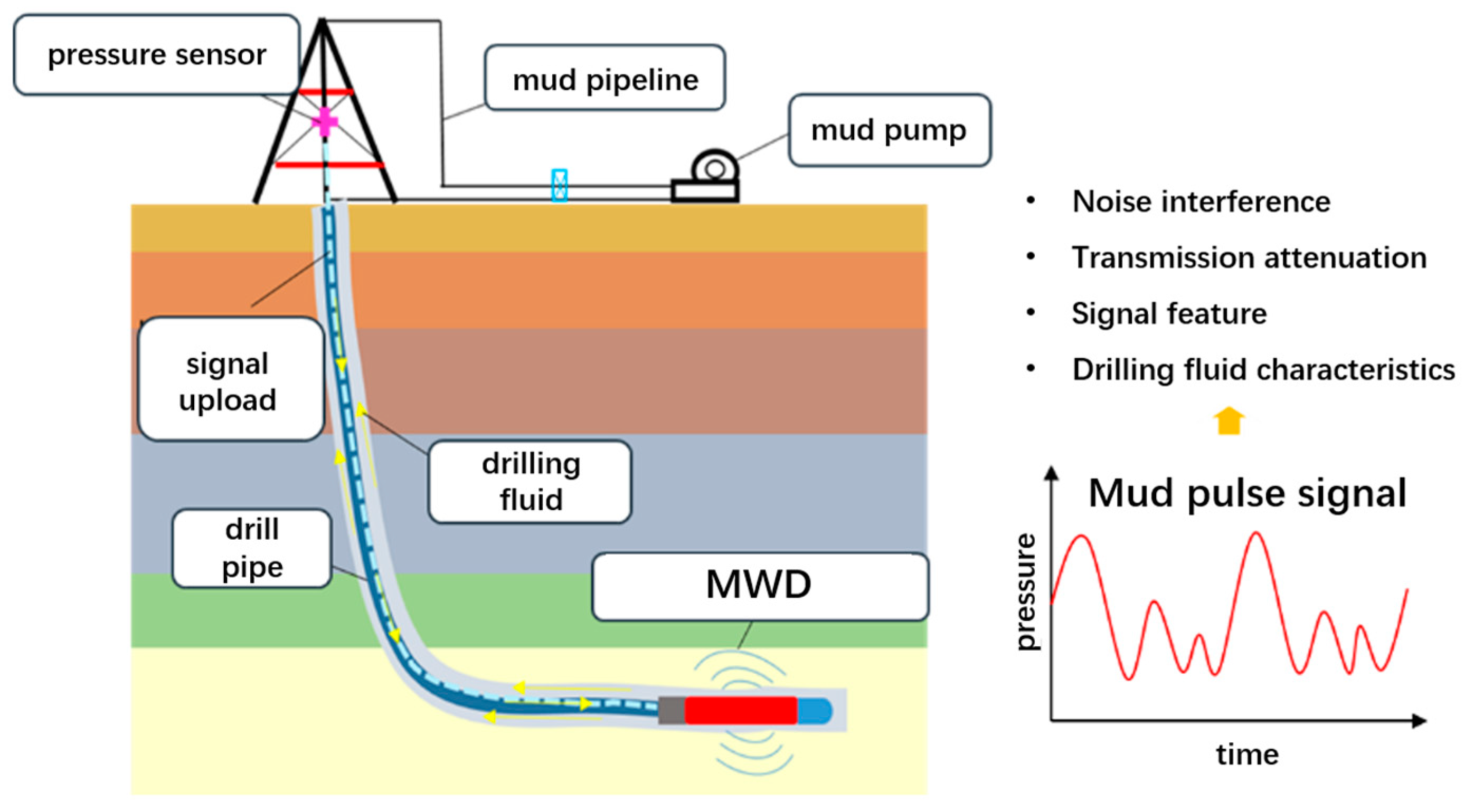
Similar to MWD technology, the mechanical measurement method also uses the hydraulic channel within the drill string to transmit signals. The drilling fluid pulse transmission method is relatively mature and can operate stably in the field [8,9,10]. The transmission of a mud pulse signal is shown in Figure 1; the basic process involves using specialized measurement techniques or mechanical structures, leveraging the instantaneous flow change during pump initiation to replace the synchronous signal bit of the electronic mud pulse generator. When the surface decoding software detects an abrupt change in pressure value, it begins demodulating the mud pulse signal. Due to varying well inclinations, the posture of the bias control center in the measurement device changes, affecting the flow area of the channel within the drill string. As the slug valve sequentially passes through annular spaces of different areas, it generates a series of continuous pulses with pressure amplitude differences as designed. These pulses combine to form the modulated signal encoding structure [11,12]. Since the information sent from the well bottom is modulated and closely related to the downhole mechanical structure, and given the spatial limitations and stability requirements of the mechanical structure, it is not possible to add synchronous and check bits to the signal as electronic measurement systems to ensure the completeness of downhole information. Therefore, the signal processing method of electronic measurement systems cannot be directly embedded. Thus, for the specific signals generated by mechanical measurement devices, distinguishing and demodulating the signals from interference after long-distance downhole transmission is particularly crucial. The main challenges lie in handling noise and identifying signals [13,14,15].

Figure 1.
Mud pulse signal transmission diagram.
Among the challenges and difficulties in the signal processing of mechanical measurement technology are the following:
- Difficulty in signal recognition
The signals generated by mechanical measurements are typically mechanical displacements or forces, which must be converted into readable electrical signals. This conversion process involves challenges in signal processing and amplification.
- 2.
- Wear and tear of mechanical components
Over extended periods of use, mechanical components may wear out, affecting the accuracy and stability of signal generation.
There are numerous classic cases in the field of mechanical measurement instrument research. For instance, National Oilwell Varco (NOV) designed an inclination-only MWD system called “Teledrift” for complex vertical wells [16]. The Teledrift measurement-while-drilling tool is a purely mechanical system that uses positive mud-pulsing technology to provide inclination for vertical downhole drilling. The tool is made of robust materials to promote longevity in the field and minimize washing from mud flow, enabling longer, more accurate runs [17]. However, Teledrift can only measure an inclination of up to 10.5° and requires a further lift [18]. Lei Li et al. [19] proposed a design method for a decimal mud pulse amplitude modulation signal, which significantly improves data transmission efficiency but lacks detailed demodulation methods. Amplitude modulation signal demodulation is often employed in fault diagnosis, and these demodulation methods can provide valuable insights into the amplitude demodulation of mud pulse signals. Common amplitude demodulation analysis methods include Hilbert envelope demodulation, generalized detection, and filtering demodulation [20]. Yuanzheng Li [21] based on the Hilbert transform, square demodulation, and least squares optimization algorithm, proposed an accurate amplitude demodulation method, achieving the reconstruction of real amplitude modulation signals.
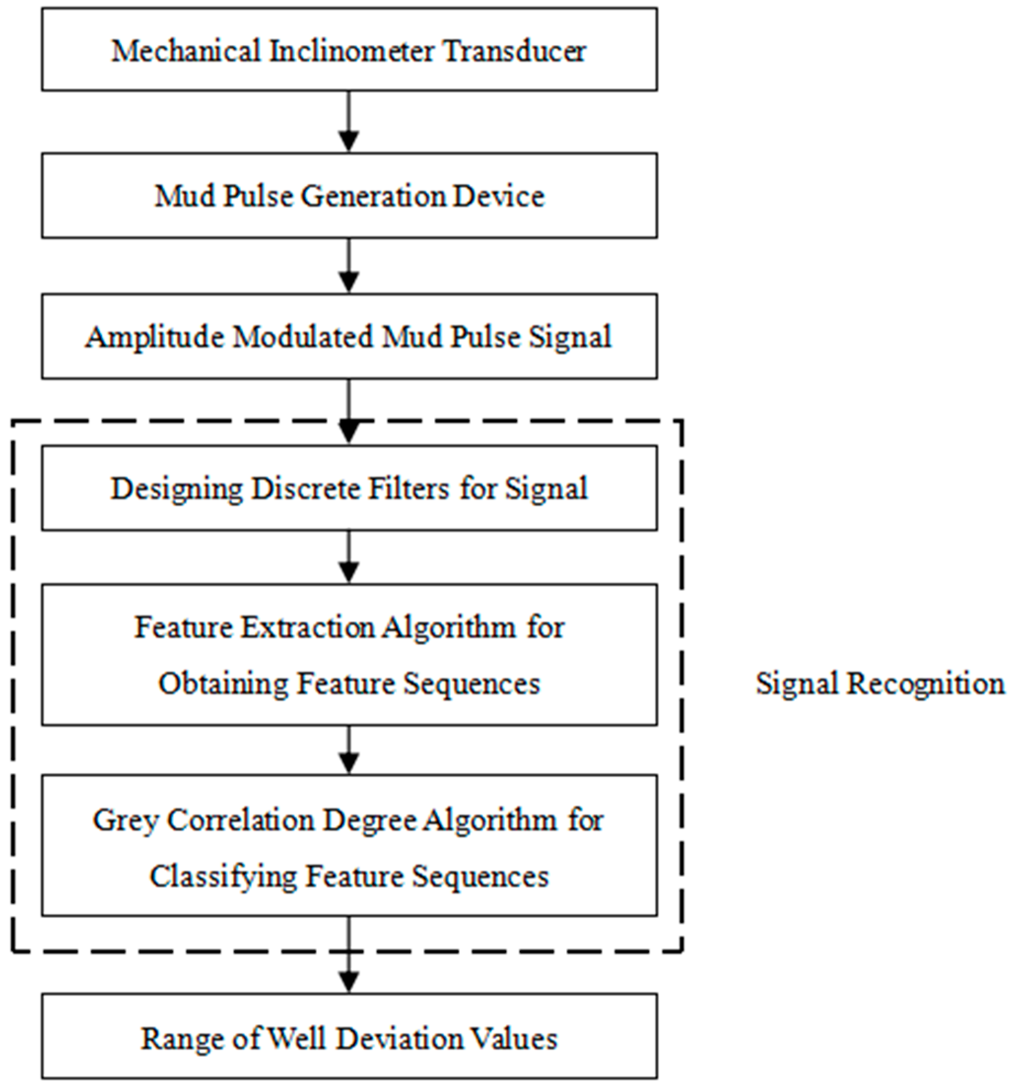
In summary, the positive pulse signals used in conventional mechanical measurements have lower transmission efficiency compared to amplitude-modulated signals. Therefore, studying how to recognize and demodulate the amplitude-modulated signals generated by mechanical measuring instruments is of significant importance. To address these issues, this paper proposes a method for recognizing and demodulating amplitude-modulated signals based on the amplitude-modulated signals generated by purely mechanical measuring instruments. According to the signal modulation method and its corresponding encoding structure, this approach includes three main analysis methods: signal filtering processing, extraction of relevant features, and classification of signal feature sequences using the grey relational analysis algorithm. The goal is to provide theoretical guidance for the transmission of mud pulse signals in ultra-deep wells up to 10,000 m deep. The developed process for identifying amplitude-modulated mud pulse signals is illustrated in Figure 2.
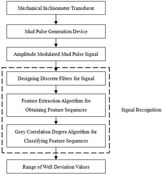
Figure 2.
Method flowchart.
2. Research on Mud Pulse Signal Recognition Algorithm
2.1. Establishment of Signal Recognition Model
The essence of mud pulse signals lies in the compressibility of the transmission medium, which creates an instantaneous pressure difference in the flow channel during the opening and closing process. If the controllable pressure difference follows a certain pattern and is easily detectable, a signal system can be constructed to transmit information. By generating pressure pulses downhole, the pressure changes in the flow channel can be recorded and detected by pressure sensors at the riser. If the detected pressure pulse patterns match the designed patterns, it indicates that the signal transmission system between the downhole and the surface has been successfully established.
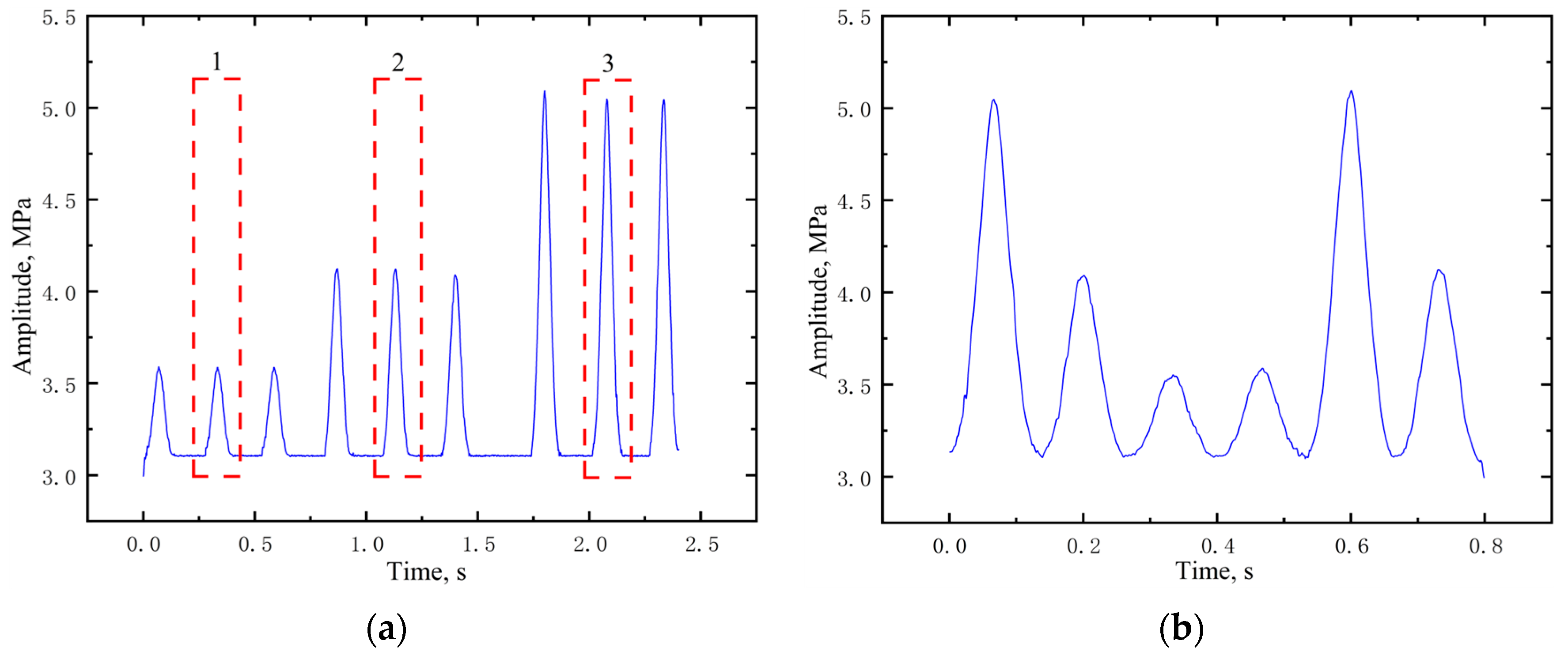
The signal recognition algorithm proposed in this paper achieves signal recognition and decoding based on the degree of matching between the detected patterns and the designed patterns. The signal modulation and design patterns are illustrated in Figure 3a. The pulse generation structure of the inclinometer tool can produce three types of pressure pulses with significant amplitude differences, corresponding to three encoding numbers. This simple, direct, and reliable modulation method is referred to as amplitude modulation. The pressure pulse combinations used to embed the inclination information are depicted in Figure 3b.
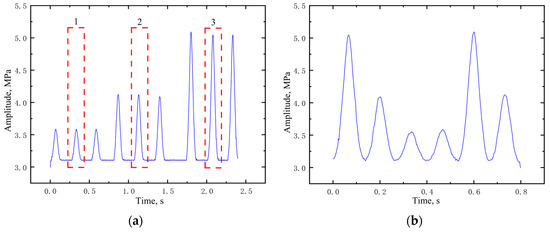
Figure 3.
Theoretical signal: (a) Amplitude pulse modulation; (b) Composite signal at well deviation of 41°–50°.
The composite signal waveform can be represented as follows:
In the equation, p(t) denotes a pulse with a duration of t. Am is the signal to be transmitted, typically encoded over two continuous cycles. In this context, Am is represented by the sequence {1, 1, 3, 2, 3, 2, 1, 1, 3, 2, 3, 2}. Xk and Xk+n are the elements of the signal to be transmitted. n is the number of pulses in a single cycle of the designed signal. Here, n is set to 6, and k is controlled by the measurement parameters, calculated as shown in Equation (2).
In the equations, x is defined as α/10, and k = [x] represents the floor function, where for any x, the condition [x] ≤ x < [x] + 1 holds true. Here, α represents the well inclination.
From Equations (1) and (2), it can be observed that when the well inclination falls within a specific range, the pulse generation structure will be influenced by the well inclination, resulting in the generation of corresponding pulse combination signals. The relationship between the types of encoding sequences represented by the combined pressure pulses and the well inclination parameters is presented in Table 1.

Table 1.
Pulse code sequences and corresponding well deviation parameters.
2.2. Noise Analysis
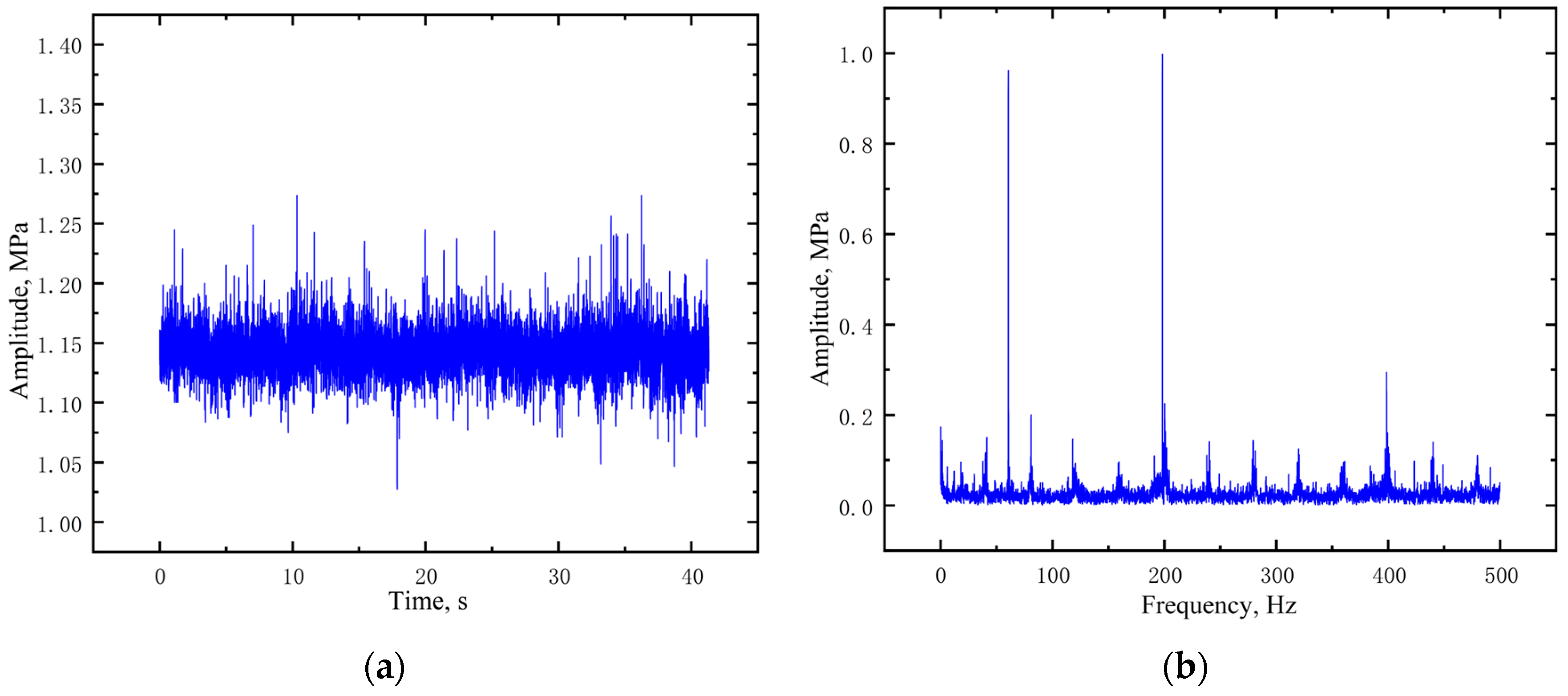
Mud pulse signals experience considerable interference when transmitted through hydraulic channels. This interference arises due to the attenuation of pulse intensity over long distances as the signal travels from the well bottom to the surface, as well as the presence of irregular pulse noise within the signal [22]. The primary source of noise interference is the mud pump, which generates noise within the same frequency range as the signal [23]. This interference can lead to signal instability and potential signal masking.
Figure 4 displays the time-domain waveform and frequency distribution of pressure noise collected from laboratory experiments. The noise frequency prominently exhibits two main frequencies, centered at 60 Hz and 200 Hz. To minimize the impact of noise, the signal generation frequency can be designed to be considerably lower than the noise frequencies. Additionally, a low-pass filter can be employed to mitigate the effects of noise.
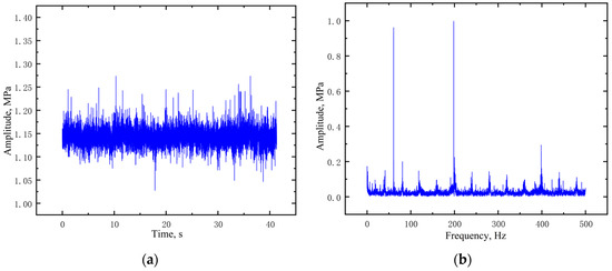
Figure 4.
Noise waveform and spectrum: (a) Time domain waveform; (b) Frequency spectrum.
2.3. Signal Processing Algorithm
2.3.1. Discrete Random Signal Filtering Algorithm
The transfer function of a continuous-time filter is expressed as:
where H(s) is the filter’s frequency-domain transfer function, s is the complex frequency variable, and τ is the filter’s time constant.
By applying the inverse Laplace transform to Equation (3), we can obtain the time-domain response of the filter:
where h(t) is the unit impulse response of the filter, and u(t) is the unit step function.
To convert this continuous-time filter into discrete time, a difference equation is used to approximate its behavior. Using the Euler method, the difference equation for the filtered output signal is derived as follows:
where O(i) is the filter’s output signal, I(i) is the filter’s input signal, F is the filter’s coefficient, and O(i − 1) is the filter’s output signal at the previous time step.
The filter coefficient F in Equation (5) can be expressed as:
where τ is an adjustable parameter where larger values result in a slower response and smaller values result in a faster response; T is the sampling frequency in Hz.
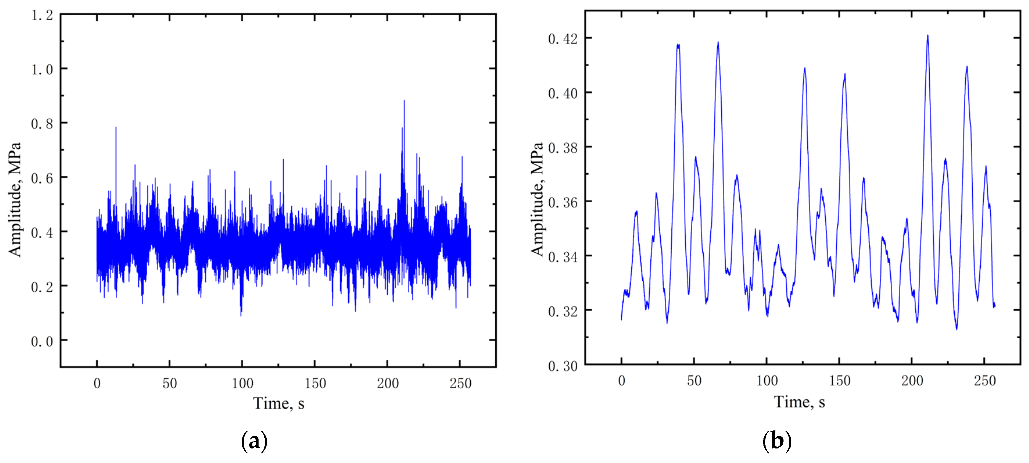
Equation (5) represents the difference equation for the discrete-time filter, where F is used to weight the current input signal and the previous output signal, taking the place of the continuous-time filter’s time constant τ; (1 − F) is used to attenuate the previous output signal, replacing the exponential decay factor e(–t/τ) in the continuous-time filter. Figure 5 illustrates a comparison of the waveforms before and after applying the discrete-time filter to remove signal noise, demonstrating that the noise is effectively eliminated from the signal.
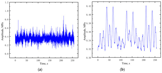
Figure 5.
Signal before and after processing comparison diagram: (a) Raw signal; (b) Processed signal.
2.3.2. EMD Signal Filtering Algorithm
Empirical Mode Decomposition (EMD) is a signal processing method utilized to decompose a complex signal into a set of intrinsic mode functions (IMFs). EMD is an adaptive, data-driven approach capable of accommodating signal structures of varying scales, thereby decomposing the signal into components with differing frequencies and amplitudes.
The fundamental concept behind EMD is to break down the signal into a series of IMFs, each exhibiting distinct frequency and amplitude characteristics, which can then be combined to reconstruct the original signal. The EMD process involves the following steps:
- Extraction of extremum points
Identify the local maxima and minima within the original signal.
- 2.
- Interpolation for IMF construction
Interpolate and connect the neighboring extremum points to create upper and lower envelopes, forming the initial set of IMFs.
- 3.
- Extraction of IMFs and residuals
Subtract the initial IMFs from the original signal to derive a series of residuals. Repeat the above steps until the residuals satisfy a specified convergence criterion.
- 4.
- Iterative refinement
Perform iterations on the IMFs and residuals obtained in each round until the termination condition is met.
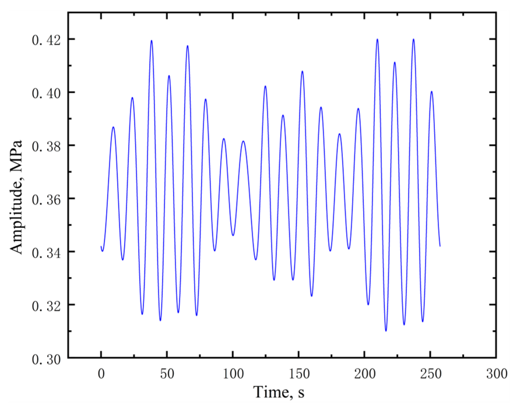
The primary advantage of EMD is its independence from pre-specified basis functions; rather, it adaptively decomposes the signal based on its intrinsic characteristics. The performance of the EMD signal filtering algorithm in processing the original signal is depicted in Figure 6. Compared to discrete random signal filtering algorithms, the EMD method is more effective in suppressing mud pump noise and can significantly identify the amplitude of valid pulse signals. Therefore, the EMD signal filtering algorithm will be used to remove signal noise in subsequent studies.
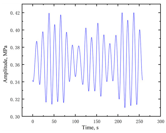
Figure 6.
Signal after filtering with EMD signal processing algorithm.
2.4. Signal Feature Extraction
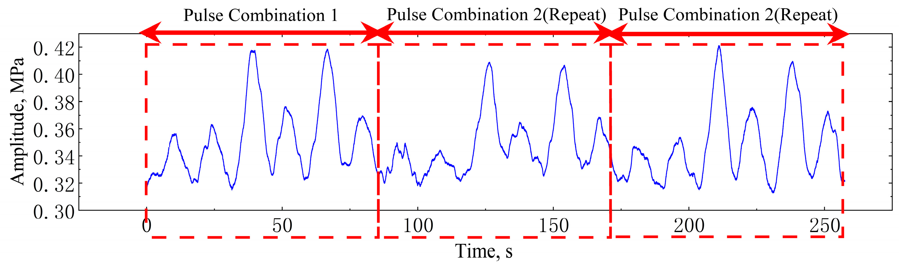
After the mud pulse signal is denoised, the encoding features within the signal become significantly more prominent, which in turn makes the signal easier to decode. An analysis of the encoding format of a single downhole signal collection reveals that, to ensure stable signal generation, the signal is repeatedly output, and the results of multiple repeated outputs are treated as a single signal segment to be decoded. As depicted in Figure 7, each signal segment for decoding consists of three identical pulse combinations, with the latter two pulse combinations being continuous repetitions of the first pulse combination.
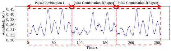
Figure 7.
Segment of signal to be identified.
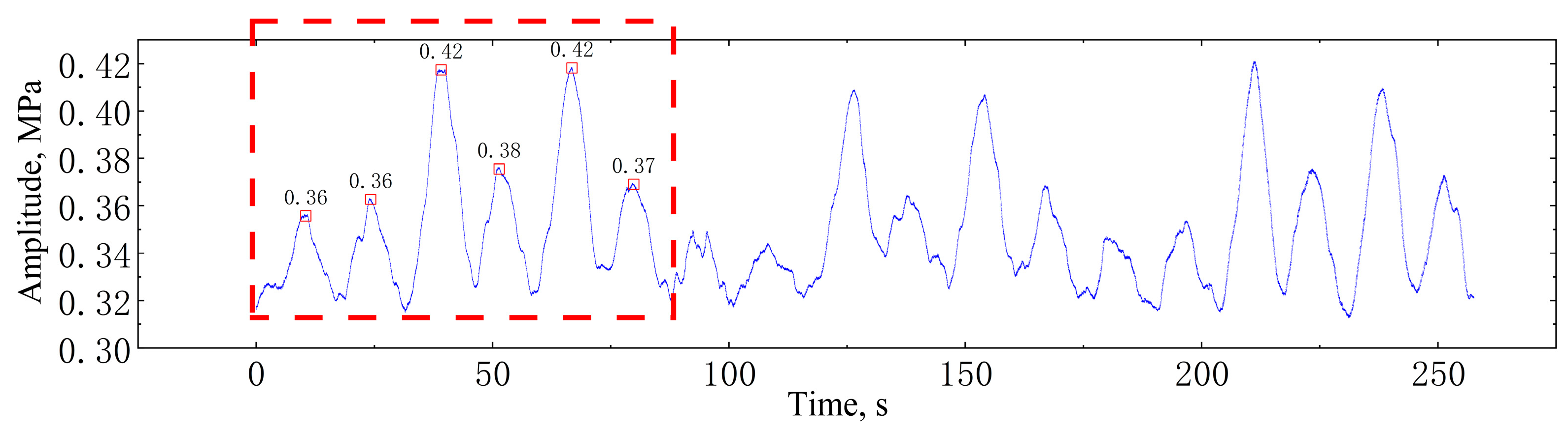
In each signal segment, all peak values are extracted to form a numerical sequence, which serves as the recognition feature of the pulse signal. Because of the repetitive nature of signal data, the first six values of the peak value sequence are employed as the identification interval during signal decoding. The peak value sequence within this interval is extracted as the feature sequence, as illustrated in Figure 8.
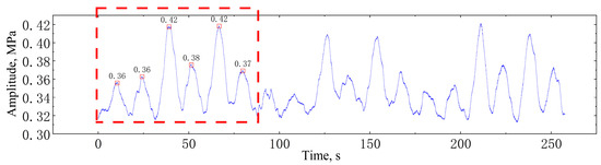
Figure 8.
Identification interval and feature extraction of the signal to be identified.
The extraction results of signal features in Figure 8 are presented in Table 2. The sequence comprising six eigenvalues is simplified, encapsulating all the information of the signal segment to be recognized. This sequence can subsequently undergo classification using pattern recognition methods for signal decoding.
Table 2.
Signal feature extraction results.
2.5. Classification of Feature Groups Using Grey Relational Analysis Algorithm
The Grey Relational Analysis (GRA) algorithm examines the connections among data by converting data sequences into grey sequences and computing their relational degrees [24,25]. In this study, GRA is applied to compare the feature amplitude sequence of the signal to be identified with different theoretical structural feature amplitude sequences of the target signal. This approach eliminates the need for repeated comparisons of individual amplitude values and can identify the pattern most similar to the signal to be recognized.
- Establishment of the pattern library matrix
Define the set of amplitude sequence patterns as X = (X1, …, Xi, …, Xn) and the set of time-domain sequence encodings as Y = (Y1, …, Yj, …, Ym). The pattern library matrix is then constructed as follows:
- 2.
- Data initialization transformation
As the amplitude values measured under various cyclic pressure conditions possess distinct dimensions, it becomes imperative to mitigate their influence on the recognition model. This objective is accomplished through the construction of an initialized amplitude sequence matrix denoted as O, for the signal undergoing identification. Correspondingly, the values within the pattern library matrix R undergo an identical initialization transformation process.
- 3.
- Calculation of the grey relational coefficient matrix
To compute the grey relational coefficients, the elements oij from the initialized signal matrix O serve as the comparison sequence, while the elements rij from the initialized pattern library matrix R serve as the reference sequence. The grey relational coefficient is determined using the following formula:
- 4.
- Maximum relational degree coefficient
By ranking the maximum relational coefficients from each row of the grey relational coefficient matrix C, the sequence corresponding to the highest value in the pattern library is identified as the recognition result sequence for the sequence to be identified. For example, the sequence to be identified in Table 2 is compared with six types of patterns in the pattern library. After performing grey relational calculations, the relational coefficients for each pattern are shown in Table 3. The “inclination 1°–10°” pattern has the highest relational coefficient, making it the most reliable decoded result for the signal.
Table 3.
Calculating grey correlation coefficients between the sequence to be identified and various pattern sequences.
3. Results Analysis and Discussion
3.1. Recognition Results of Simulated Signals
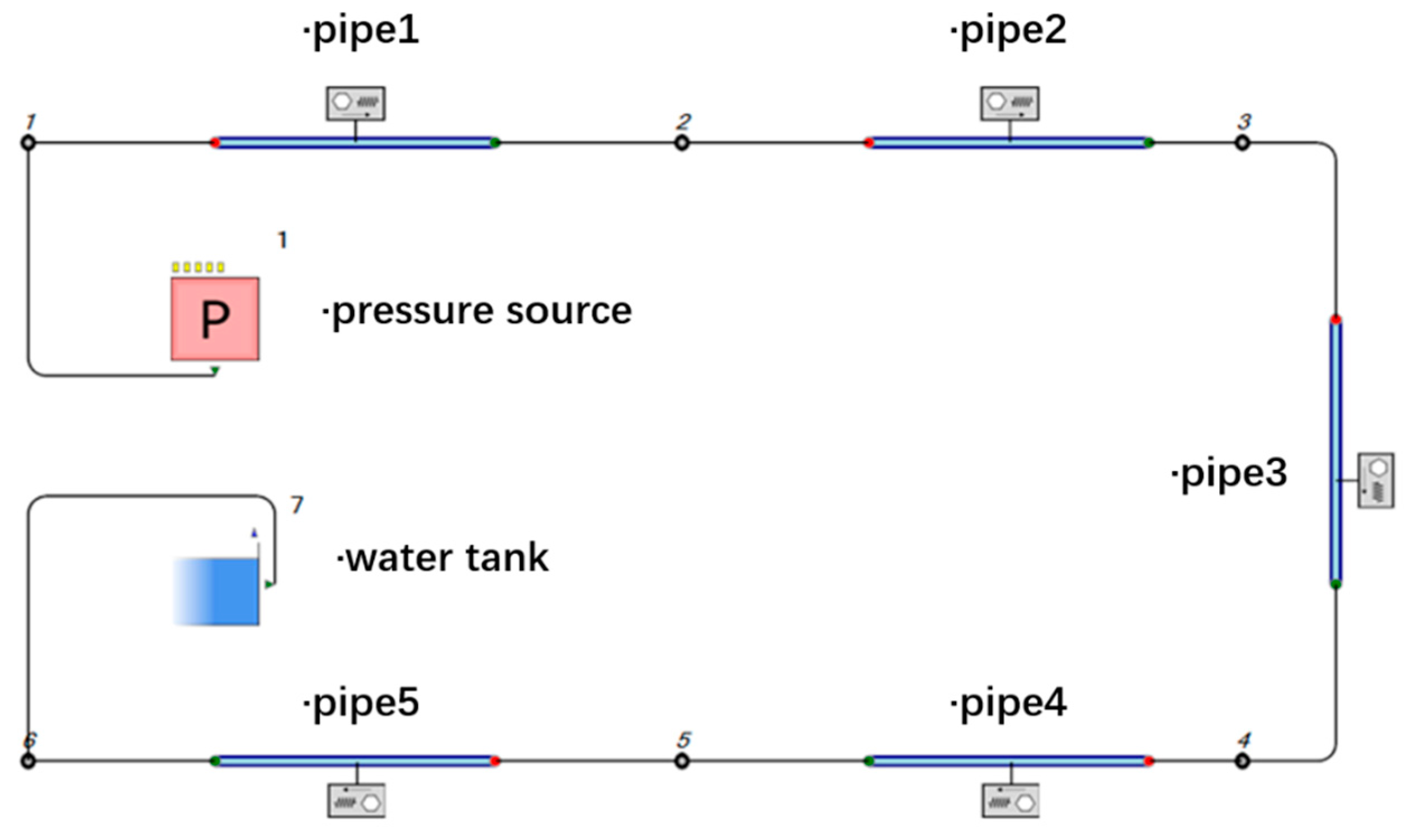
The amplitude characteristics of mud pulse signals often experience substantial attenuation as the transmission distance increases. Furthermore, noise interference during the transmission process can lead to distortions in the encoded waveform received on the surface. To validate the recognition accuracy of the designed algorithm, a simulation analysis pipeline for long-distance signal transmission was developed, depicted in Figure 9.
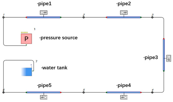
Figure 9.
Pipeline for simulation analysis of long-distance signal transmission.
In general, the relationship between the intensity of continuous pulse signals and the transmission distance during the transmission of mud pulse signals can be analyzed using Lamb’s law, which is expressed as follows:
where p is the intensity of the pulse signal in Pascals (Pa), p0 is the initial intensity of the pulse signal in Pascals (Pa), x is the transmission distance in meters (m), L is the attenuation factor, which is the transmission distance at which the pulse signal attenuates to 1/e of its initial intensity in meters (m). The attenuation factor L is given by:
where f is the frequency of the pulse signal, f = ω/2π, ω is the angular frequency of the pulse signal, c′ is the transmission rate (m/s), D is the diameter of the pipeline (m), ρ is the density of the mud (kg/m3), and μ is the viscosity of the mud (Pa·s).
However, the above conventional method for analyzing the attenuation of mud pulse signal transmission primarily focuses on the reduction in signal amplitude during transmission. It overlooks factors such as interference between upward and downward waveforms, pipeline characteristics, and the coupling effects of various mud properties. To address these aspects, pipeline water hammer analysis software was utilized to establish a long-distance transmission analysis pipeline for mud pulse signals. In this analysis, the designed waveform data are inputted into the pressure source component. The mud pulse signal transmission speed is set at 1200 m/s, with clear water used as the external fluid. Relevant parameters of the pipeline are detailed in Table 4.
Table 4.
Simulation system transmission pipeline parameters.
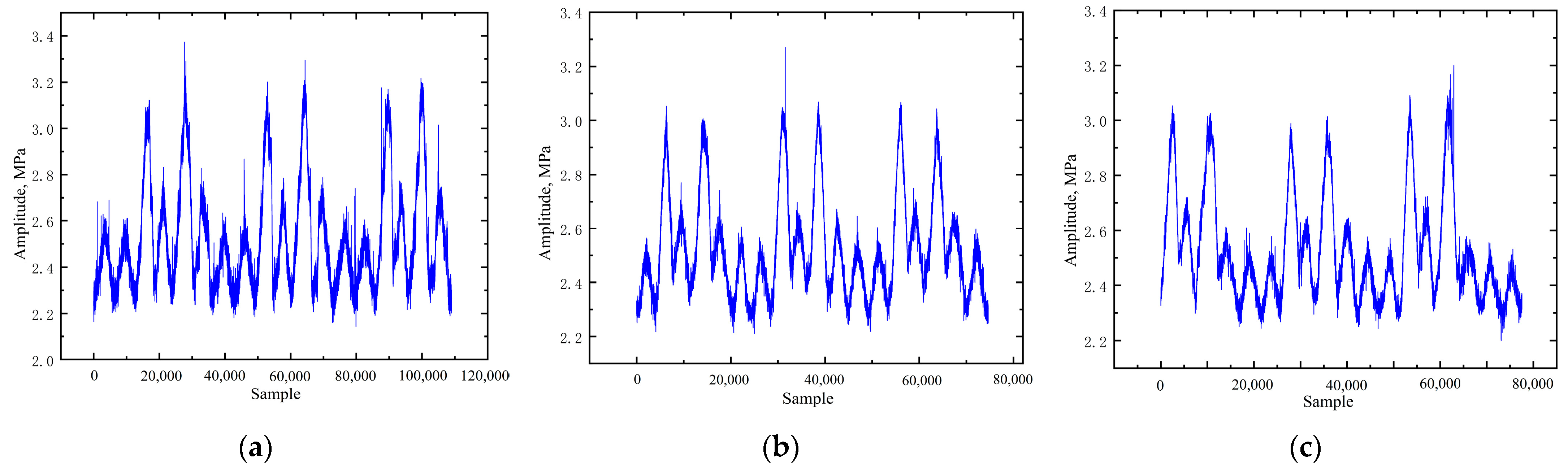
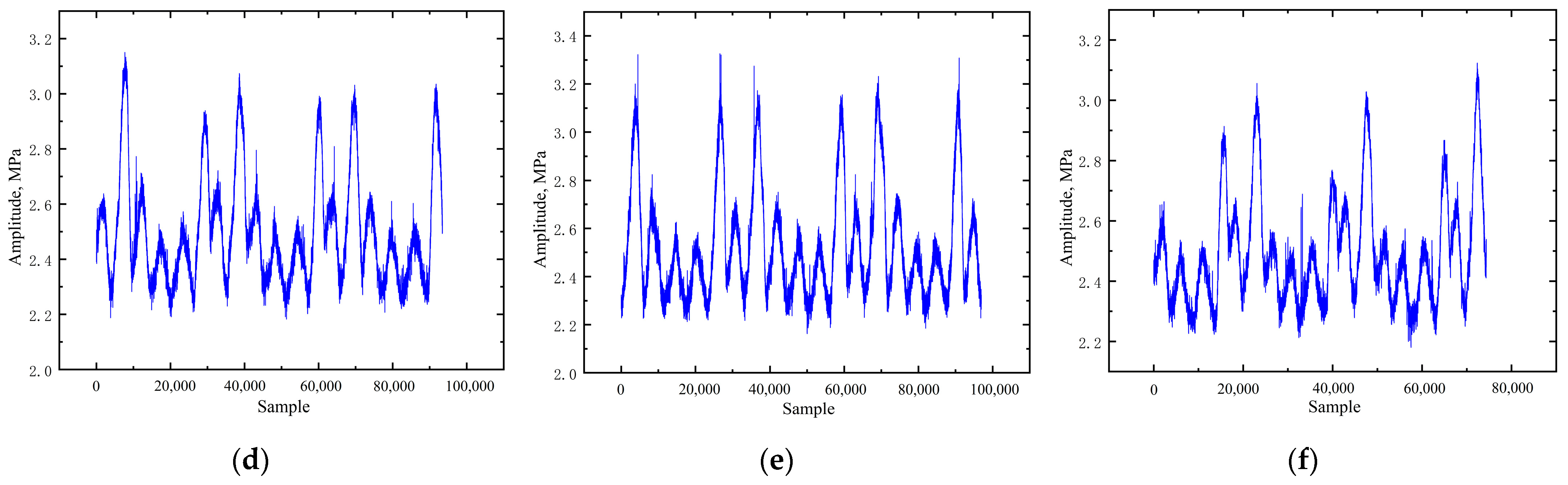
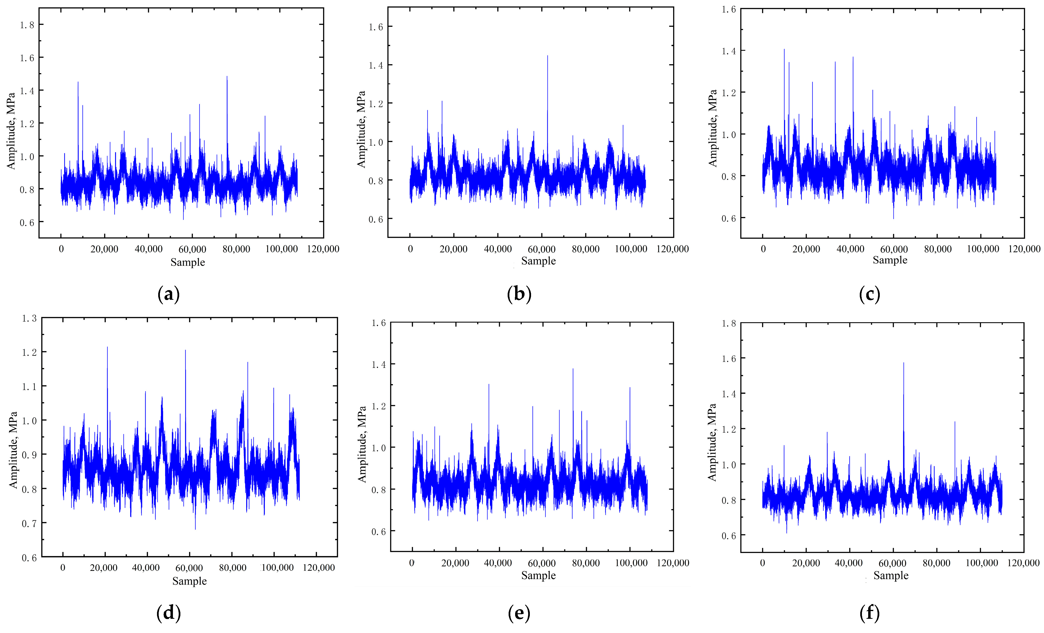
Gaussian noise was introduced into the simulated signals, Figure 10 and Figure 11 display the characteristic waveform curve of the simulated signal post 500 m and 10,000 m of transmission, respectively. Notably, distinct changes in the waveform post-transmission are observable, indicating a high resolution in pulse differential pressure.
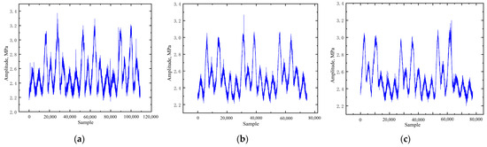
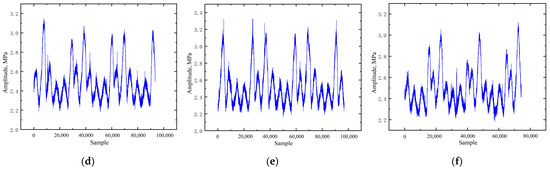
Figure 10.
A 500-m transmission simulation signal diagram: (a) inclination 5°; (b) inclination 15°; (c) inclination 25°; (d) inclination 35°; (e) inclination 45°; (f) inclination 55°.
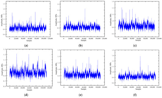
Figure 11.
A 10,000-m transmission simulation signal diagram: (a) inclination 5°; (b) inclination 15°; (c) inclination 25°; (d) inclination 35°; (e) inclination 45°; (f) inclination 55°.
Firstly, it is evident that the amplitude intensity of the simulated signal at 10,000 m is considerably lower compared to that at 500 m; the increase in transmission distance results in a noticeable attenuation of signal strength. Furthermore, the presence of noise diminishes the clarity of the encoded waveform features, thereby increasing the difficulty in signal recognition. Specifically, the “1” encoding experiences amplitude attenuation and distortion. The recognition algorithm was employed to analyze the recognition results of the signal, which were then statistically summarized and are presented in Table 5. Remarkably, even after transmission over a distance of 10,000 m, all six groups of simulated signals were correctly identified.
Table 5.
Simulation signal identification results.
3.2. Recognition Results of Indoor Experimental Data
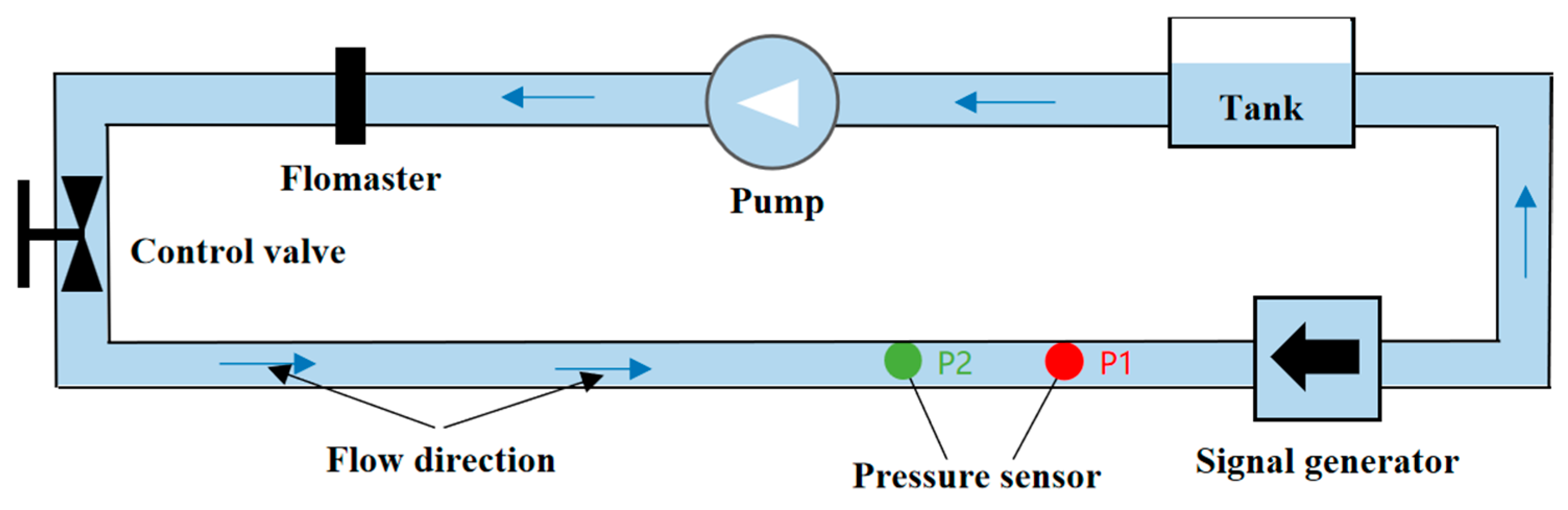
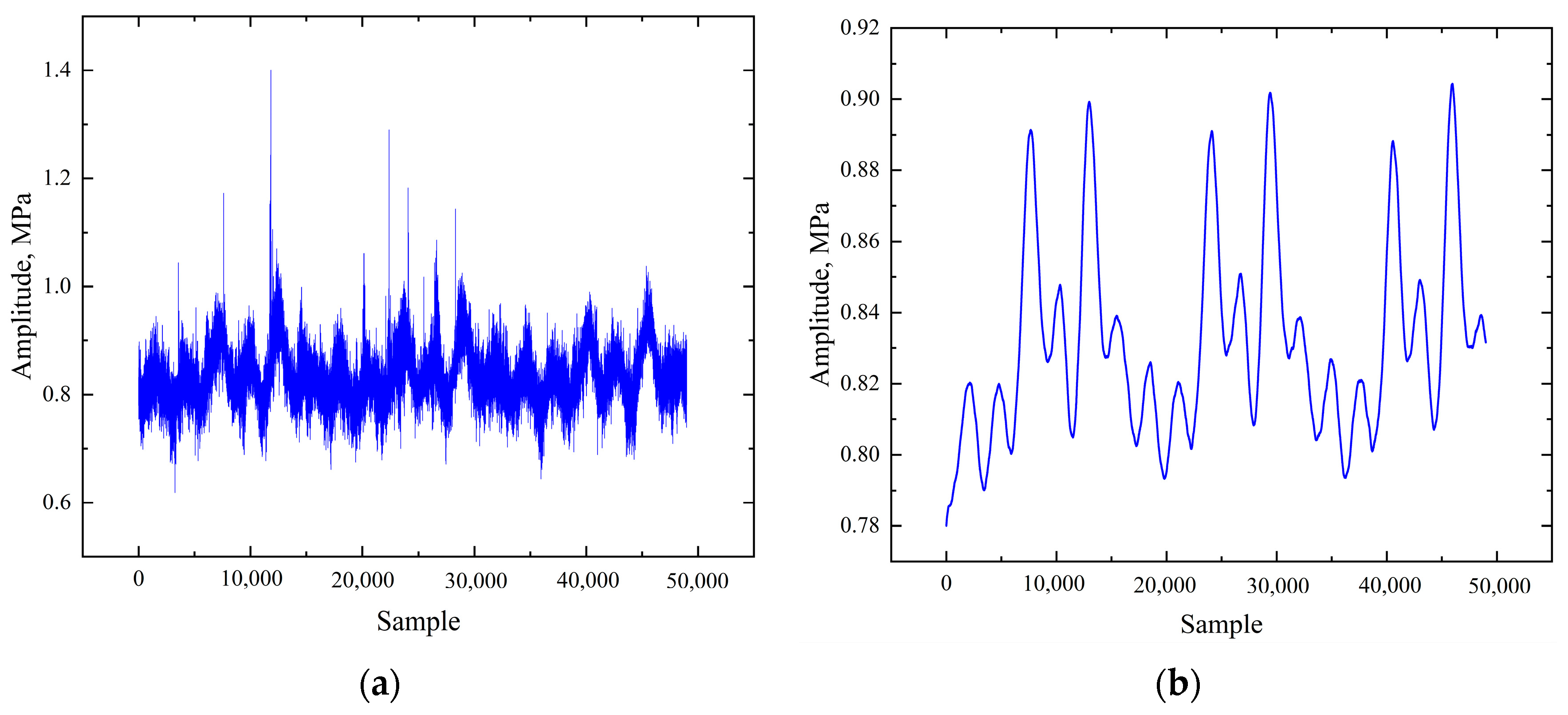
Subsequently, we constructed the platform illustrated in Figure 12 to conduct indoor experiments, further validating the applicability and recognition accuracy of the designed algorithm. The experimental setup included a tank, pump, Flomaster, and control valve, with careful consideration given to the impact of mud pump noise on pulse signals. To ensure comprehensive data collection, the experimental system includes two pressure sensors. Pressure sensor P1, positioned near the pulse generator was utilized to capture mud pulse signals, while pressure sensor P2 served as a backup. The inclination was set from 5° to 55°, conducting experiments at intervals of 10°. Filtering was applied to the pulse signals collected by the pressure sensor. Figure 13 illustrates the raw and filtered signals at inclinations of 5°, with schematic diagrams of signals at other inclinations provided in Appendix A.

Figure 12.
Indoor experimental system schematic diagram.
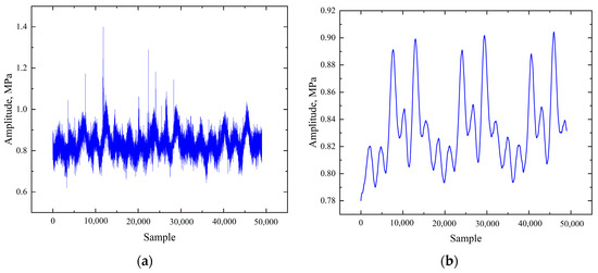
Figure 13.
Indoor experimental signal diagram: (a) Raw signal with 5° inclination; (b) Processed signal with 5° inclination.
Due to noise interference, the individual peaks of the signal were heavily distorted. The outcomes of the grey relational analysis are detailed in Table 6.
Table 6.
Grey correlation calculation results.
The grey relational coefficients across the six modes exhibit relative proximity, with the “Inclination 1°–10°” mode showing the highest coefficient. This indicates that this mode is the closest to the experimentally measured signal. Moreover, the actual inclination angle represented by the signal is 5°, falling within the degree range of the mentioned mode. Consequently, the recognition outcome is deemed accurate. The analysis results presented above validate that the method of extracting signal features simplifies the signal processing procedure, as evidenced by both simulated and indoor experimental signals. Employing the grey relational analysis algorithm for signal pattern recognition and classification facilitates convenient and reliable interpretation of the information embedded within the signals.
4. Conclusions
This study has developed a signal encoding and demodulation algorithm specifically for mechanical inclinometer instruments. Through an analysis of the composition structure of the signal encoding, as well as signal processing and feature extraction, a feature group model has been established. This model effectively constructs a recognition method for amplitude-encoded signals in ultra-deep wells of up to 10,000 m. The method’s validation has been conducted through simulations and experiments. The following conclusions can be drawn from the research on signal recognition methods:
- (1)
- Through an analysis of the structure of mud pulse amplitude modulation signals, the selection of appropriate filtering methods significantly enhances the signal-to-noise ratio. This amplifies the prominence of signal features and facilitates subsequent analysis using recognition methods.
- (2)
- Utilizing the peak characteristics of signal pulses as the basis for identification and constructing a feature group sequence model with consecutive peak features simplifies the signal during identification. This simplification results in enhanced identification efficiency.
- (3)
- By employing grey relational analysis to classify peak feature sequences for signal decoding, a systematic signal recognition method applicable to the field of mud pulse amplitude modulation signal recognition is achieved. The feasibility of this recognition method has been validated through signal recognition tests conducted in indoor experiments.
5. Future Directions
There are still many limitations and deficiencies in the study, which need to be improved in future work:
- (1)
- The pulse coding sequence corresponds to the range of inclination angle, which represents a limitation in our current work. Teledrift has already managed to control the accuracy within a range of 0.5° to 1.5° [18], and we aim to further improve the precision of pulse recognition to meet this standard.
- (2)
- Current research has primarily focused on the measurement of inclination angles. However, there are still many critical downhole parameters that require measurement, such as azimuth, face angle, weight on bit, torque, and vibration. Therefore, we plan to enhance the comprehensiveness of our approach to enable accurate measurement of these additional parameters.
- (3)
- Furthermore, in future work, we will continue to conduct experimental research, thoroughly considering the impact of white noise on pulse recognition. Additionally, we will validate the accuracy of our methods using mud pulse signals detected in the field.
Author Contributions
Conceptualization, Q.W. and G.J.; methodology, Q.X.; software, Q.X.; validation, Q.W. and G.J.; formal analysis, K.W.; investigation, C.M.; resources, L.Z.; data curation, J.G.; writing—original draft preparation, Q.X.; writing—review and editing, Q.W.; visualization, J.G.; supervision, J.G.; project administration, K.W.; funding acquisition, C.M. All authors have read and agreed to the published version of the manuscript.
Funding
This research was funded by PetroChina Key Core Technology Research Project, Research on key technology and equipment for drilling and completing 10,000-m ultra-deep oil and gas resource wells (2022ZG06).
Data Availability Statement
Data are contained within the article.
Conflicts of Interest
Authors Qing Wang, Guodong Ji, and Long Zeng are employed by the company CNPC Engineering Technology R&D Company Limited. Jianhua Guo, Ke Wu, and Chao Mei are employed by PetroChina Southwest Oil & Gasfield Company. The remaining authors declare that the research was conducted in the absence of any commercial or financial relationships that could be construed as a potential conflict of interest.
Nomenclature
| t | Duration |
| S(t) | composite signal waveform |
| p(t) | pulse with a duration of t |
| Am | signal to be transmitted |
| Xk and Xk+n | elements of the signal to be transmitted |
| n | number of pulses |
| k = [x] | floor function |
| α | well inclination |
| s | complex frequency variable |
| H(s) | filter’s frequency domain transfer function |
| τ | filter’s time constant |
| h(t) | unit impulse response of the filter |
| u(t) | unit step function |
| O(i) | filter’s output signal |
| I(i) | filter’s input signal |
| F | filter’s coefficient |
| O(i − 1) | filter’s output signal at the previous time step |
| T | sampling frequency |
| X = (X1, …, Xi, …, Xn) | set of amplitude sequence patterns |
| Y = (Y1, …, Yj, …, Ym) | set of time-domain sequence encodings |
| R | pattern library matrix |
| O | initialized amplitude sequence matrix |
| oij | elements from initialized amplitude sequence matrix |
| rij | elements from initialized pattern library matrix |
| cij | grey relational coefficient |
| C | grey relational coefficient matrix |
| p | intensity of the pulse signal |
| p0 | initial intensity of the pulse signal |
| x | transmission distance |
| L | attenuation factor |
| f | frequency of the pulse signal |
| ω | angular frequency of the pulse signal |
| c′ | transmission rate |
| D | diameter of the pipeline |
| ρ | density of the mud |
| μ | viscosity of the mud |
Appendix A
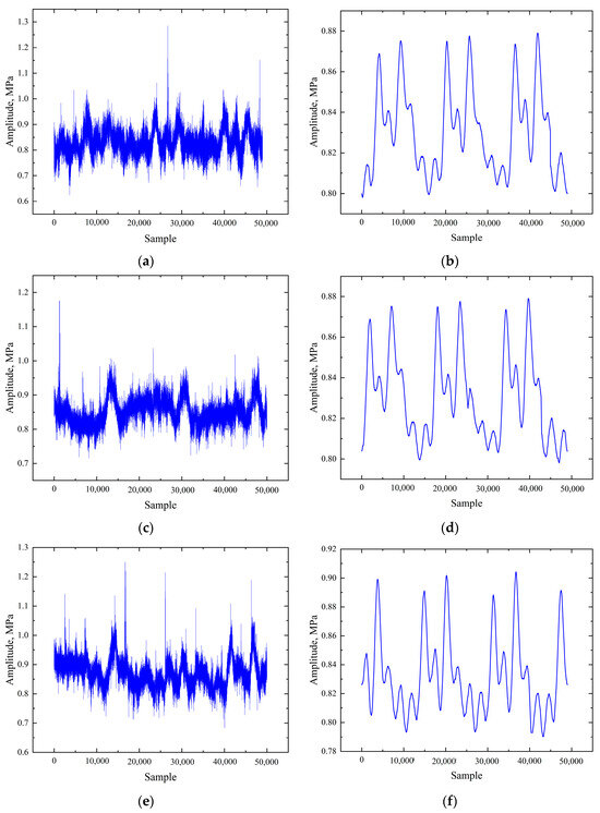
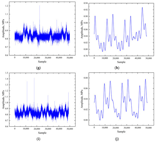
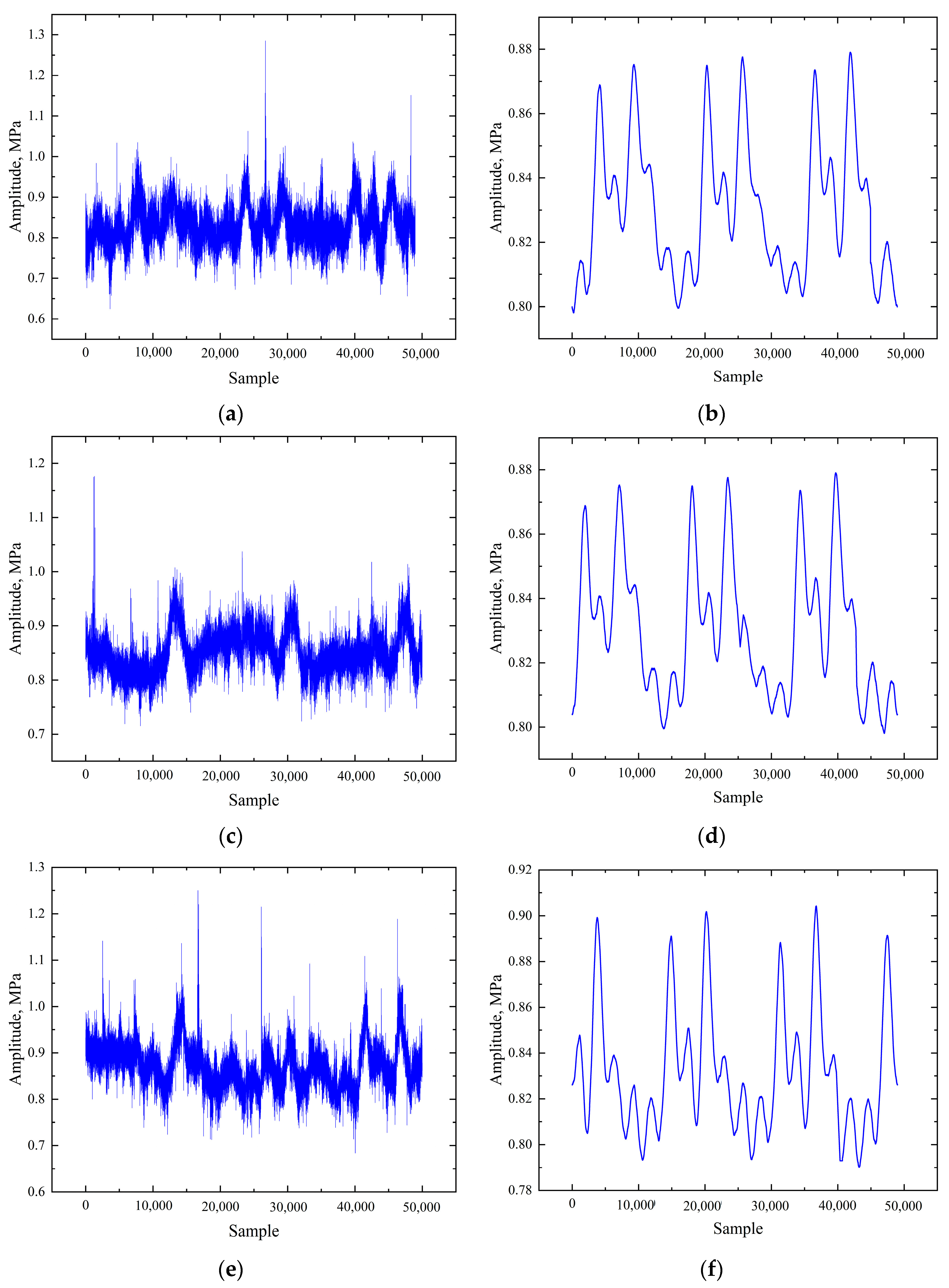
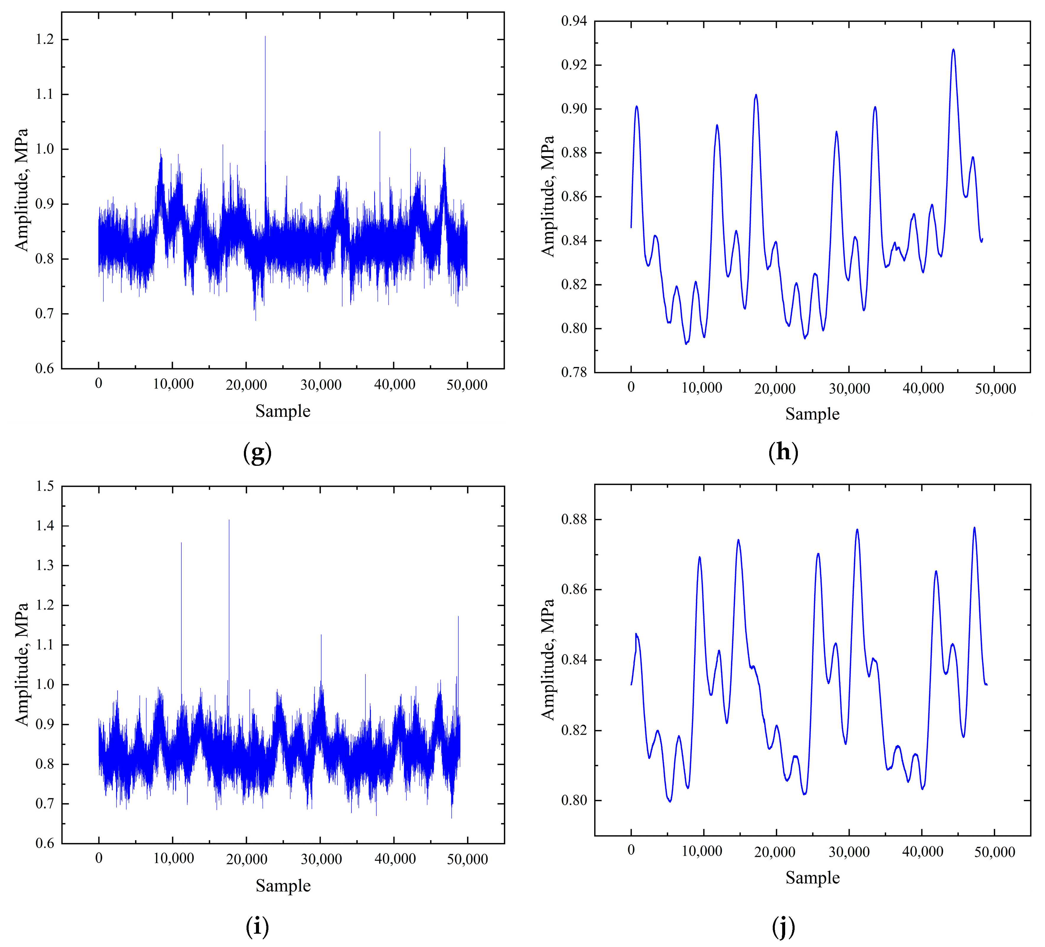
Figure A1.
Supplementary indoor experimental signal diagram: (a) Raw signal with 15° inclination; (b) Processed signal with 15° inclination; (c) Raw signal with 25° inclination; (d) Processed signal with 25° inclination; (e) Raw signal with 35° inclination; (f) Processed signal with 35° inclination; (g) Raw signal with 45° inclination; (h) Processed signal with 45° inclination; (i) Raw signal with 55° inclination; (j) Processed signal with 55° inclination.
References
- Zhang, J.; Xie, W. Status of Scientific Drilling Technology for Ultra–Deep Well. Acta Geol. Sin. 2010, 84, 887–894. [Google Scholar]
- Liu, H.; Liu, J.; Liu, H.; Qiu, J.; Cai, B.; Liu, J.; Yang, Z.; Liu, J. Progress and development direction of production test and reservoir stimulation technologies for ultra–deep oil and gas reservoirs in Tarim Basin. Nat. Gas Ind. 2020, 40, 76–88. [Google Scholar]
- NOV. Available online: https://www.nov.com/products/e-totco-electronic-drift-survey-tool (accessed on 30 July 2024).
- Peng, Q.; Li, H.; Zhang, Q. Application Status of the Technology of Logging While Drilling. Adv. Mater. Res. 2014, 3384, 1650–1653. [Google Scholar] [CrossRef]
- Tang, Z.; Zhou, J.; Zhao, H.; Li, L.; Shi, B.; Zeng, M. Measurement and control technology while drilling for ultra–deep horizontal wells in Yuanba Gasfield. Oil Drill. Prod. Technol. 2015, 37, 54–57. [Google Scholar]
- Rai, P.; Schunnesson, H.; Lindqvist, P.; Kumar, U. Measurement–while–drilling technique and its scope in design and prediction of rock blasting. Int. J. Min. Sci. Technol. 2016, 26, 711–719. [Google Scholar] [CrossRef]
- Su, Y.; Dou, X.; Gao, K.; Liu, K. Discussion and prospects of the development on measurement while drilling technology in oil and gas wells. Pet. Sci. Bull. 2023, 8, 534–535. [Google Scholar]
- Cai, W.; Wang, P.; Zhu, Y.; Chen, G. Design scheme and key techniques for mechanical wireless inclinometer. Acta Pet. Sin. 2006, 2, 103–106. [Google Scholar]
- Sun, J.; Liu, T. Improvement and application of mechanical wireless inclinometer while drilling technology. Drill. Prod. Technol. 2012, 35, 108–110. [Google Scholar]
- Liu, X. Research on Mechanism of Continuous Wave Signal Generator Controlled by DSP and the Wind Tunnel Simulation Test. Ph.D. Thesis, China University of Petroleum (East China), Qingdao, China, 2009. [Google Scholar]
- Mcdonald, W.J. Four Different Systems Used for MWD. Oil Gas J. 1978, 76, 115–124. [Google Scholar]
- Gearhart, M.; Moseley, L.M.; Foste, M. Current State of the Art of MWD and Its Application in Exploration and Development Drilling. In Proceedings of the International Meeting on Petroleum Engineering, Beijing, China, 17–20 March 1986. [Google Scholar]
- Liang, Y.; Ju, X.; Li, A.; Li, C.; Dai, Z.; Ma, L. The Process of High–Data–Rate Mud Pulse Signal in Logging While Drilling System. Math. Probl. Eng. 2020, 2020, 3207087. [Google Scholar] [CrossRef]
- Tu, B.; Li, S.; Lin, H.; Ji, M. Research on mud pulse signal data processing in MWD. EURASIP J. Adv. Signal Process. 2012, 2012, 182. [Google Scholar] [CrossRef]
- Mwachaka, M.; Wu, A.; Fu, Q. A review of mud pulse telemetry signal impairments modeling and suppression methods. J. Pet. Explor. Prod. Technol. 2018, 9, 779–792. [Google Scholar] [CrossRef]
- Pálsson, B.; Hólmgeirsson, S.; Guðmundsson, Á.; Bóasson, H.Á.; Ingason, K.; Sverrisson, H.; Thórhallsson, S. Drilling of the well IDDP–1. Geothermics 2014, 49, 23–30. [Google Scholar] [CrossRef]
- NOV. Available online: https://www.nov.com/products/teledrift-prodrift-mwd-tool (accessed on 30 July 2024).
- drillingforgas.com. Available online: https://drillingforgas.com/en/drilling/directional/teledrift-inclination-only-mwd (accessed on 30 July 2024).
- Li, L.; Deng, H.; Huang, C.; Zhang, J.; Xie, Y.; Wan, F.; Zeng, P.; Jia, L.; He, X.; Duan, M.; et al. Method for Siginal Transmission Based on Mud Pulse Pressure Amplitide. China Patent CN110500087A, 26 November 2019. [Google Scholar]
- Zhang, F.; Ding, K. Research on the Three Algorithms and Limitations of Generalized Detection Filtering Demodulation Analysis. J. Vib. Eng. 2002, 2, 123–128. [Google Scholar]
- Li, Y. Research on Demodulation Method of Gear Fault Vibration Amplitude and Frequency Modulation Signal. Master’s Thesis, South China University of Technology, Guangzhou, China, 2021. [Google Scholar]
- Qu, J.; Xue, Q.; Lu, J. Analysis on the change characteristics of waveform during the transmission of continuous wave mud pulse signal. Alex. Eng. J. 2023, 80, 594–608. [Google Scholar] [CrossRef]
- Chen, G.; Yan, Z.; Gao, T.; Sun, H.; Li, G.; Wang, J. Study on model–based pump noise suppression method of mud pulse signal. J. Pet. Sci. Eng. 2021, 200, 108433. [Google Scholar] [CrossRef]
- Deng, J. Grey System Theory Tutorial; Huazhong University of Science & Technology Press: Wuhan, China, 1990; pp. 21–24. [Google Scholar]
- Zhang, J.; Zhang, Q.; Zhang, J. The result greyness problem of the grey relational analysis and its solution. J. Intell. Fuzzy Syst. 2023, 44, 6079–6088. [Google Scholar] [CrossRef]
Disclaimer/Publisher’s Note: The statements, opinions and data contained in all publications are solely those of the individual author(s) and contributor(s) and not of MDPI and/or the editor(s). MDPI and/or the editor(s) disclaim responsibility for any injury to people or property resulting from any ideas, methods, instructions or products referred to in the content. |
© 2024 by the authors. Licensee MDPI, Basel, Switzerland. This article is an open access article distributed under the terms and conditions of the Creative Commons Attribution (CC BY) license (https://creativecommons.org/licenses/by/4.0/).