A Methodology for Efficient Antenna Deployment in Distributed Massive Multiple-Input Multiple-Output Systems

Abstract

This paper, taking as reference channel data previously obtained by using a rigorous and well-tested ray-tracing method for a concentrated massive multiple-input multiple-output (mMIMO) system, focuses on the optimization of the set of potential antennas required in a distributed mMIMO system to achieve the same channel spectral efficiency as the concentrated system. Concerning the optimizer, a binary particle swarm optimization algorithm was considered to decide whether to activate or deactivate any of the antennas within the original mesh, taking into account, in order to direct the search, the total spectral efficiency, the equality between the spectral efficiency of users, and the number of receiver antennas at the distributed base station. The analysis was carried out in a large indoor environment at the 5G n258 frequency band (26 GHz), concentrating on the up-link and considering a set of 20 uniformly distributed active users. The results obtained show that, in the distributed mMIMO system, an arrangement with fewer than half the number of receiver antennas of the initial mesh is required to achieve a similar performance to that of the concentrated one taken as a reference.

1. Introduction

The evolution from classical point-to-point multiple-input multiple-output (MIMO) technology towards multiuser massive MIMO (mMIMO) has become an enabling technology in the development of applications and services in 5G mobile networks [1,2]. The future technical evolution of the mMIMO concept is still considered one of the most promising technologies in the development of 6G and beyond due to its great potential [3,4]. There are some technical limitations of the multicell co-located mMIMO concept: the difficulty of grouping a large number of antennas concentrated in a single location, the base station (BS), and the unequal coverage and increased interference at the cell edge.

These drawbacks, together with the emergence of the concept of decentralized networks [5], has led to the hybridization of both concepts through the idea of distributed mMIMO (D-mMIMO) systems. In contrast to BSs based on concentrated mMIMO (C-mMIMO), this technology distributes a large number of antennas over a large area, so that the entire BS antenna array surrounds each terminal, rather than having the UTs surrounding the BS, as in the classical cellular concept [6,7]. A new evolution of these ideas from the point of view of the architecture network subject to intensive research at present is the concept of ultra-dense cell-free massive MIMO, which can be seen as an evolution of the user-centric network MIMO concept [4].

Focusing on the physical layer, a comparative analysis between the C-mMIMO and D-mMIMO channel characteristics is of great interest. Numerous theoretical studies have been reported in the literature for a decade [8,9,10,11]. From an experimental point of view, there are few studies, and some worth highlighting include [12,13,14,15]. In all these studies, the potential advantages of D-mMIMO systems over C-mMIMO are revealed. Several recent studies carried out by the authors have also shown the advantages of D-mMIMO over C-mMIMO systems [16,17]. In [16], channel measurements carried out in indoor environments at 3.5 GHz show that D-mMIMO outperforms the C-mMIMO system in terms of sum capacity, spectral efficiency, and user fairness. Moreover, in [17], a comparison between C-mMIMO and D-mMIMO channels at 26 GHz in an indoor environment using ray tracing (RT) [18] shows that the D-mMIMO channel outperforms the C-mMIMO one in terms of channel capacity, showing a mean channel capacity of 11 bit/s/Hz higher than in C-mMIMO. The RT method used in [17], and by extension in this work, is a well-tested channel simulator through measurements that has been previously used for characterizing MIMO channels [18]. In addition, it has also been used together with heuristic methods to optimize the deployment of wireless local area networks [19].

In 5G, the strategic deployment of networks to meet the requirements of different usage scenarios has received great attention, and proposals introducing optimization tools have emerged in the literature as solutions for such complex optimization tasks. For instance, in [20], metaheuristic algorithms are successfully applied to optimize cell deployment in hyper-dense 5G networks. More recently, in [21], a methodology to optimize the positioning of base stations in 5G networks, maximizing coverage and data rates while minimizing deployment expenses, is presented. In this case, different metaheuristics, such as genetic algorithms (GAs), particle swarm optimization (PSO), simulated annealing, and grey wolf optimizer, are used as the optimization tool, and their performance is evaluated and compared. In [22], an approach to optimize power allocation in 5G device-to-device communications can be found and, in [23], a multi-objective GA-based approach is applied to reduce power consumption in 5G networks. Moreover, in [24], the idea of neural networks is extended to optimize cell-free mMIMO networks.

In mMIMO systems, optimum antenna array deployment is of great importance, as it contributes not only to improving coverage and quality of service (QoS) for the users, but also to saving power (contributing also to the reduction in digital carbon footprint) as well as reducing the complexity of the fronthaul architecture, especially in D-mMIMO systems. In this work, we propose a methodology for efficient antenna deployment in D-mMIMO systems. Starting from the generally accepted fact that D-mMIMO outperforms the C-mMIMO system in terms of total spectral efficiency and user fairness, the motivation and contribution of this paper focus on finding the answer to the following question: considering a maximum number of antennas for both systems, concentrated and distributed, how many and which antennas from the potential set are required in the distributed system to match the performance of the concentrated one? The answer to this question, as will be shown, leads to a significant reduction in the antennas needed in the distributed system compared to the concentrated one. The solution to the question is posed as an antenna selection problem, a subject that has received much attention in C-mMIMO systems and, lately, also in D-mMIMO systems [25,26,27,28]. The novelty of the methodology presented in this paper lies in the fact that, for a specific indoor environment, the method proposed makes it possible to optimize the set of antennas necessary in the D-mMIMO system to meet certain channel requirements, which is useful prior to network deployment. Concerning the optimization issue, a modified version of the classical binary PSO [29] has been considered in this work [30]. The only relationship between the physical problem at hand and the PSO is established by means of a fitness function. For the optimization problem presented, the fitness function to be minimized takes into account the differences in the cumulative distribution function (CDF) over the full frequency band of both the spectral efficiency and the equality between the spectral efficiency of the users (fairness), as well as the number of active antennas required in the D-mMIMO system to match the performance of the C-mMIMO one. In spite of the fact that the authors consider as channel metrics to optimize the D-mMIMO system those reference values obtained for the C-mMIMO one in the same scenario, the approach presented in this work could consider any other values or indicators of QoS required.

The main contributions of this work are summarized as follows:

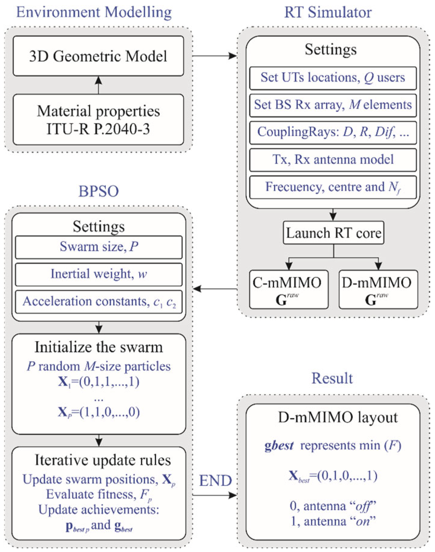
• A methodology for efficient antenna deployment in D-mMIMO systems is presented. The method is site-specific and relies on the combination of RT for channel characterization with a metaheuristic optimization-based approach.
• Starting with a maximum number of potential active antennas, the method proposed makes it possible to optimize, i.e., reduce, the set of antennas necessary in the D-mMIMO system to meet certain channel requirements.
• The fitness function to be minimized takes into account the differences in the CDFs along the full frequency band for both spectral efficiency and fairness; therefore, the optimization considers the wideband nature of time-division duplex orthogonal frequency-division multiplexing (TDD-OFDM) schemes.
• The methodology leads to a significant reduction in the antennas needed in the distributed system compared to the concentrated one.
• It is a flexible approach in which any other QoS indicators can be considered, making it possible to modulate the search by modifying the fitness function if desired.

The remainder of this paper is organized as follows: Section 2 presents the methodology, including the theory of the mMIMO channel model, the role of ray tracing in the channel matrix computation, and the D-mMIMO optimization approach, showing the relationship between the problem at hand and the optimizer. The results obtained in a large indoor cell are presented and discussed in Section 3, and, finally, Section 4 summarizes the main conclusions that can be drawn from this work.

2. Methodology

2.1. Up-Link Massive MIMO Model

Let us consider the up-link of a single-cell mMIMO system consisting of M antennas at the BS and Q single-antenna user terminals (UTs) in the cell, as shown in Figure 1 for both C- and D-mMIMO systems. Basically, in the classical concentrated system, the BS serves the UTs using a large number of antennas. In contrast, in the cell-free or distributed mMIMO system, there are many BSs surrounding the UTs that are jointly serving these UTs. In this case, a central processing unit is required to centralize and carry out signal processing. In D-mMIMO, each BS can be equipped with one (as considered in this work) or multiple antennas. Concerning other formal aspects of the model, let us consider that the UTs transmit a total power of P and do not collaborate with each other; it is also assumed that the BS knows the channel (perfect channel estimation) and that we consider an OFDM system with N_f sub-carriers. Under these assumptions, the received signal at the BS for the k-th sub-carrier when the Q users are active is a 1 × M vector given by the following:

$$\mathbf{y}\left[k\right]=\sqrt{SNR}\mathbf{G}\left[k\right]\mathbf{s}\left[k\right]+\mathbf{n}\left[k\right];\hspace{1em}k=1,2,\cdots ,N_f,$$

(1)

where SNR is the mean signal-to-noise ratio at the receiver, G[k] is a channel matrix of size M × Q in which every column corresponds to the narrowband channel g_q[k] (M × 1); s[k] of order Q × 1 represents the signal vector transmitted by the users, which is normalized so that E{‖s‖²} = 1; and n[k] is a complex Gaussian noise vector with independent and identically distributed (i.i.d.) unit variance elements.

The channel matrix G is normalized so that it satisfies (2) and is obtained from (3) using the raw channel matrix associated with the scenario and layout under analysis, denoted as G^raw:

$$E\left\{{‖\mathbf{G}‖}_F^2\right\}=M\cdot Q,$$

(2)

$${\mathbf{G}}_{M\times Q}={\mathbf{G}}_{M\times Q}^{raw}{\mathbf{J}}_{Q\times Q}.$$

(3)

In (2), ‖·‖_F represents the Frobenius norm, and the G^raw channel matrix in (3) is obtained in this work using RT simulations, as described below in Section 2.2. Moreover, the normalization matrix J in (3) is a diagonal matrix of order Q × Q whose elements are given by the following [31,32]:

$$j_q=\sqrt{{\displaystyle \frac{M}{\frac{1}{N_f}{\displaystyle \sum _{k=1}^{N_f}{\left|g_q^{raw}\left[k\right]\right|}^2}}}};\hspace{1em}q=1,\cdots ,Q.$$

(4)

According to (4), the power imbalance between the channels linked to each UT is removed, but the variations in the channels between antennas at the receiver array and across frequency tones are preserved. The normalized matrix G can be understood as representing a system in which ideal power control is implemented. The total available power transmitted by the UTs is not evenly distributed, yet all UTs arrive at the base station with the same mean power.

The received signal is processed at the receiver using a linear combination technique like zero-forcing (ZF), so the combination matrix is given by the following:

$$\mathbf{V}=\mathbf{G}{\left({\mathbf{G}}^H\mathbf{G}\right)}^{-1}.$$

(5)

The signal processed at the receiver can be represented as follows:

$$\hat{\mathbf{s}}\left[k\right]={\mathbf{V}}^H\left[k\right]\mathbf{y}\left[k\right],$$

(6)

in which $\hat{\mathbf{s}}\left[k\right]$ (1 × Q) represents the estimation of the signals transmitted by the Q UTs for the k-th frequency tone.

The signal-to-interference-plus-noise ratio (SINR) of the q-th user on the k-th sub-carrier is given by (7), with the individual spectral efficiency (SE) of each user calculated using (8), and, finally, the sum SE is determined according to (9).

$$SIN{R}_q\left[k\right]={\displaystyle \frac{\frac{SNR}{Q}{\left|{\mathbf{V}}_q^H{\mathbf{g}}_q\right|}^2}{\frac{SNR}{Q}{\displaystyle \sum _{i=1,i\ne q}^Q{\left|{\mathbf{V}}_q^H{\mathbf{g}}_i\right|}^2+{\left|{\mathbf{V}}_q\right|}^2}}},$$

(7)

$$S{E}_q\left[k\right]={\log }_2\left(1+SIN{R}_q\left[k\right]\right),$$

(8)

$$SE\left[k\right]={\displaystyle \sum _{q=1}^{Q}S{E}_q\left[k\right]}.$$

(9)

Finally, user fairness, given by Jain’s fairness index (JFI) [33], has also been considered as a metric to quantify the fairness of the channel in sharing the SE among the UTs:

$$JFI=E\left\{{{\displaystyle \frac{\left({\displaystyle \sum _{q=1}^{Q}S{E}_q\left[k\right]}\right)}{Q{\displaystyle \sum _{q=1}^{Q}S{E}_q^2\left[k\right]}}}}^2\right\},$$

(10)

where E{·} denotes the mathematical expectation computed over the N_f sub-carriers. JFI takes values between 1/Q and 1, with the value 1 representing the maximum fairness.

2.2. Channel Matrix Using Ray Tracing

A ray-tracing tool based on a full three-dimensional (3D) implementation of geometrical optics, along with the uniform theory of diffraction (3D GO/UTD) [18], was used by the authors to obtain the raw channel matrix for both concentrated and distributed mMIMO systems considered.

The simulator uses as reference a 3D geometric model of the propagation environment consisting of flat facets, along with electrical parameters for every facet (representing a wall, the floor, ceiling, or specific scatterers such as cabinets or doors), including its conductivity, relative dielectric constant, either the transmission coefficient or the plate’s width, and the standard deviation of the surface roughness. Concerning the radio propagation process modeling, the software tool represents it through a set of user-selectable scattering mechanisms, so the coupling between both transmitter (Tx) and receiver (Rx) antennas is the result of the contribution of different rays: direct field (D), multiple reflections (from the first order, R, up to the tenth order, R¹⁰), and single and double edge diffractions (Dif and Dif², respectively), as well as combinations of reflection–diffraction (R-D) and diffraction–reflection (D-R).

Let us consider an arbitrary propagation environment in which a set of N rays connect both Tx and Rx antennas. The RT simulator makes it possible to directly obtain the channel impulse response and, making use of the Fourier transform, the channel transfer function at a given frequency can be obtained as follows:

$$H\left(f\right)={\displaystyle \underset{-\infty }{\overset{\infty }{\int }}{\displaystyle \sum _{i=1}^N{a}_i\delta \left(\tau -{\tau }_i\right)}{e}^{-j2\pi f\tau }d\tau =}{\displaystyle \sum _{i=1}^N{a}_i}{e}^{-j2\pi f{\tau }_i},$$

(11)

where a_i represents the complex voltage induced on the receiver antenna by the i-th ray, and τ_i is its associated arrival time. The result in (11) is a scalar, and according to the mMIMO model presented in Section 2.1, it corresponds to the radio channel established between a certain q-th transmitter or UT and the m-th antenna element at the BS at the k-th frequency sub-carrier; i.e., considering the k-th sub-carrier, H(f) corresponds to every element g_m,q that makes up the raw channel matrix G^raw in (3). Therefore, in summary, taking as reference a certain environment and mMIMO cell layout, the RT tool is used in this work to obtain the G^raw channel matrix.

2.3. D-mMIMO Optimization Aproach

Let us suppose a certain environment in which a D-mMIMO system aims to be deployed, and let us consider a large number of potential locations for the BS antennas. In short, the task involves finding the optimal set of active antennas necessary at the D-mMIMO BS, among such a potential set of antenna locations, to meet certain QoS requirements. In this work, the target QoS values taken as reference to carry out the optimization are those that would be achieved with a BS of the C-mMIMO system deployed in the same environment and strategically placed to obtain the best results. However, the approach proposed is flexible, and any other QoS criteria can be considered if desired. The approach proposed by the authors consider channel parameters, such as the achievable SE and JFI already presented in Section 2.1, as the main QoS metrics. Furthermore, the optimal planning requires rewarding those solutions involving the lowest number of active antennas, as they would contribute to reducing both the complexity and power consumption of the network.

For the multimodal antenna selection task proposed, an improved binary version of the classical PSO algorithm (BPSO) [29,34] has been considered in this work [30]. Basically, the PSO algorithm is a metaheuristic optimization method inspired by the social behavior of swarms such as bird flocking or fish schooling [34], in which a swarm of particles or potential solutions direct the search by cooperation and competition among the individuals, influenced by their past and present experience along with their partners’ past experience.

Concerning the workflow of the BPSO algorithm, let us take a swarm with P particles, and for each particle p, the M-dimensional vector X_p = (x₁,…, x_M) is used to represent its position. Elements in X_p take values of 0 or 1, indicating that an antenna of D-mMIMO must be “off” or “on”, respectively. Moreover, let us denote as p_best p and g_best two 1 × M row vectors representing the best location, i.e., potential solution, ever found by the p-th particle and by the whole swarm, respectively. Let us introduce two velocity vectors for each particle, denoted as ${\mathrm{V}}_p^b$, where the superscript b can take values of 0 or 1, representing the probability of the bits of the particle to change to 0 or 1. Focusing on the m-th bit of the p-th particle, each element of ${\mathrm{V}}_p^b$ is calculated and iteratively updated as follows:

$$v_{p,m}^b=w{v}_{p,m}^b+{\psi }_3\left[c_1{r}_1\left({\psi }_1-p_{best p,m}\right)\right.+c_2{r}_2\left({\psi }_2-g_{best,m}\right),$$

(12)

where w is the inertia weight, c₁ and c₂ are acceleration constants that determine how the memory of both the particle and the whole swarm influence the probability of change [34], r₁ and r₂ are two independent random numbers U[0, 1], ${\psi }_1=\overline{p_{best p,m}}$ and ${\psi }_2=\overline{g_{best, m}}$ represent the 1’s complement of the m-th bit, and, finally, ψ₃ is a constant that takes a value of 1 if b = 0 and −1 when b = 1 [30]. An upper bound, V_max, is placed on the velocity in all dimensions to balance the exploration of the search space, so the result in (12) is limited according to (13) and then normalized using (14), in which s(v) is the sigmoid function. V_max in (13) is often set to 4.0 to prevent saturation of the sigmoid function [29]:

$${v^{\prime }}_{p,m}^b=\mathrm{sign}\left(v_{p,m}^b\right)\min \left\{\left|v_{p,m}^b\right|,V_{max}\right\}$$

(13)

$${v^{″}}_{p,m}^b=\mathrm{s}\left({v^{\prime }}_{p,m}^b\right)={\displaystyle \frac{1}{1+e^{-{v^{\prime }}_{p,m}^b}}}.$$

(14)

Finally, the update rule of each element (bit) in X_p from iteration i to i + 1 is given by the following:

$$x_{p,m}\left(i+1\right)=\left\{\begin{array}{c}\overline{x_{p,m}\left(i\right)},\hspace{1em}if{r}_3<{v^{″}}_{p,m}^b\\ x_{p,m}\left(i\right),\hspace{1em}if{r}_3>{v^{″}}_{p,m}^b\end{array}\right.,$$

(15)

in which r₃ is a random number U[0, 1], ${v^{″}}_{p,m}^1$ must be considered if $x_{p,m}\left(i\right)=0$, and ${v^{″}}_{p,m}^0$ must be considered in case $x_{p,m}\left(i\right)=1$.

The accuracy of each particle or potential solution, X_p, is evaluated using a fitness function that links the optimizer to the physical problem under analysis. In this sense, taking as reference the mMIMO system presented in Section 2.1, consisting of Q UTs and M antennas at the BS, the CDF of both SE and JFI can be computed using (9) and (10), taking advantage of the G^raw data previously obtained using the RT tool for both concentrated (used as reference) and distributed (under the X_p proposed layout) mMIMO systems. Finally, the fitness function proposed to be minimized and used to evaluate the accuracy of each particle is given by the following:

$$F_p=w_1\left|{\displaystyle \sum _{k=1}^{N_f}\left({\mathbf{SE}}_C[k]-{\mathbf{SE}}_{D,p}[k]\right)}\right|+\left|{\displaystyle \sum _{k=1}^{N_f}\left({\mathbf{JFI}}_C[k]-{\mathbf{JFI}}_{D,p}[k]\right)}\right|+{\displaystyle \sum _{m=1}^M{\mathbf{X}}_p\left(m\right)}.$$

(16)

In (16), the first and second terms represent the errors in both SE and JFI for the whole frequency band, where the subscripts C and D are associated with C- and D-mMIMO, respectively. The third term corresponds to the number of active antennas in the p-particle, rewarding those solutions with the lowest number of antennas. In the initial tuning of the cost function, it was observed that, for an arbitrary particle, p, the contribution to the total error in (16) of the first summand was about three orders of magnitude above the contribution to the error of the other two summands. If the first term in (16) is not properly scaled, the optimizer considers neither the optimization of the JFI nor of the number of antennas in the distributed system. That is the reason why the weight w₁ is introduced in (16), used to balance the influence of the three terms on the fitness value, so that during the initial iterations, the two first summands in (16) are the main contributions to F_p, and both condition the exploration of the search space but, during the last iterations, the number of active antennas (third addend in (16)) represents the main contribution to F_p.

The flowchart summarizing the whole approach is shown in Figure 2. Basically, the first block is devoted to the “Environment Modeling”, including the 3D geometric modeling of the environment, generated using, for instance, a computer-aided design (CAD) application, and completed by introducing the electromagnetic properties of the materials associated with any of the facets that make up the model. Later on, taking as reference the geometric model of the environment, the second block, i.e., the “RT Simulator”, focuses on the computation of the raw channel matrix for both mMIMO systems, concentrated and distributed. In the RT simulator software (CINDOOR v6.0), the user must place in the environment both the UTs and the BS array locations for the C- and D-mMIMO setups, and choose settings such as the multipath coupling mechanisms between the Tx and Rx antennas, the type or far-field pattern for both antennas, or details concerning the frequency band of interest. As a result, the RT tool obtains the G^raw channel matrix for the C- and D-mMIMO layouts. At this point, the optimizer now comes into play, so the third block of the flowchart summarizes the iterative process inherent in the BPSO algorithm. In summary, starting from some initial settings for the algorithm (size of the swarm, P; inertial weight, w; acceleration constants, c₁ and c₂), the whole swarm is randomly generated, where each particle will represent a potential BS D-mMIMO layout by encoding in a binary nature the state of any of its M-array elements. In an iterative process, the whole swarm is made to evolve by applying the rules outlined in (12)–(15), updating for each particle in each iteration its cost or fitness, F_p, according to (16), its memory representing the best position ever visited by the particle, p_best, and the best position/solution found by the swarm so far, g_best. When the termination criterion is met, usually given in terms of number of iterations or just once a residual error is achieved, the BPSO stops, and the position of the best particle in the swarm (g_best) points to the optimal solution for the D-mMIMO system, consisting of the best set of active antenna elements to keep active out of the initial M-element set.

The methodology proposed is modular, flexible, and scalable considering that, on the one hand, the optimizer module, i.e., the BPSO in Figure 2, can be replaced by another optimization algorithm, either a metaheuristic optimizer or an artificial intelligence (AI)-based optimization core and, on the other hand, either the fitness function given in (16) to drive the search or the reference values, i.e., the C-mMIMO SE and JFI QoS parameters used to optimize the D-mMIMO layout, can be changed to achieve other goals.

3. Results and Discussion

This section includes both representative results obtained in an indoor environment at 26 GHz with the methodology proposed, along with their associated discussion, showing the usefulness of the approach.

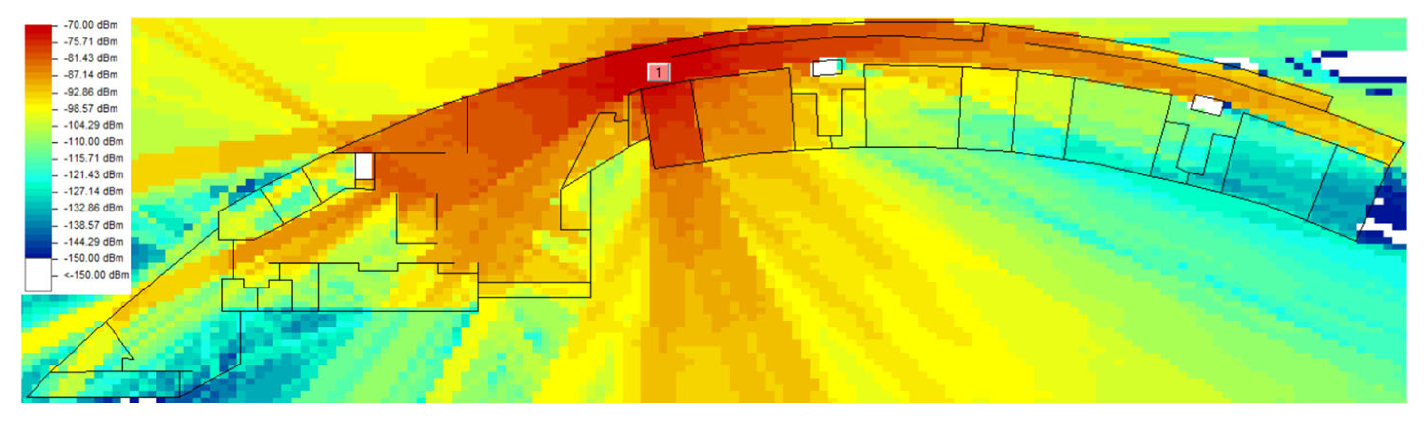
3.1. Environment and Settings

This study was carried out in the environment shown in Figure 3, corresponding to the main floor of a large building [17], including details of the position of the set of 20 UTs considered in the cell, along with the receiver arrays for both C- and D-mMIMO systems.

The C-mMIMO array is a vertical square array located at 2.5 m from the ground, consisting of 10 × 10 half-wave dipoles (M = 100) λ/2 uniformly spaced in both dimensions (0.536 λ at 26 GHz). The site of C-mMIMO was appropriately selected with the help of the RT simulator, with the intention of choosing the best location to ensure an almost homogeneous coverage throughout the environment. For this purpose, different potential locations for the C-mMIMO BS were investigated, concentrating on the down-link, considering a transmitter power of 0 dBm, half-wave dipoles at both the Tx and Rx sides, a frequency of 26 GHz, and coupling mechanisms including D, R, R², R³, Dif, and Dif² rays; and the resulting best site is that shown in Figure 4. The coverage maps presented in Figure 4 show almost homogeneous coverage, avoiding coverage holes, apart from the three local areas depicted in white and associated with the interior space of the three lifts in the building. These coverage holes are due to the fact that each one of the four flat facets used to represent the enclosed space inside each lift has been modeled as a perfect conductor, so there is no signal inside the lifts from a simulation point of view.

Concerning the D-mMIMO system, the same number of antennas (M = 100) was considered at the BS, and the potential sites allowed for these antennas were evenly distributed throughout the building floor, as shown in Figure 3. In this particular case, the antennas were placed close to the ceiling board at a height of 2.8 m, and a 3D pattern close to that of a short vertical dipole was considered in the RT simulator.

Regarding the materials to be considered in the electromagnetic modeling of the walls, floor, ceilings, and lifts in the environment, the main elements include brick, concrete, glass, and metal. Electrical properties such as their relative permittivity, ε_r, or the conductivity, σ, are summarized in

Table 1. Electromagnetic properties of the materials.

Material	εr	σ (S/m)	Use
Brick	3.91	0.0401	Walls
Concrete	5.24	0.5908	Floor, ceiling
Glass	6.31	0.2828	Front walls
Perfect conductor	1	1 × 107	Lifts

[17,35].

The analysis was carried out in the 5G n258 band, considering a bandwidth of 500 MHz (25.75–26.25 GHz) and a spacing of 60 kHz between sub-carriers, with a total of N_f = 8334 frequency tones. Finally, an average SNR equal to 10 dB was considered at each receiver array for both the C- and D-mMIMO systems.

As already stated in Section 2.3, the target channel QoS that is required to be met by the D-mMIMO system is given by the metrics provided by the aforementioned C-mMIMO system considered in this work as reference, given in terms of sum SE and JFI. In fact, according to (16) and leaving aside the influence of the number of antennas to keep active, the goal concentrates on minimizing the errors of the two first addends. In this sense, to clarify the process, it is useful to present as the starting point the optimization margin available for both SE and JFI indicators, comparing for those purposes both the C-mMIMO reference channel results and the results associated with a hypothetical D-mMIMO system in which all the 100 antennas were active. For the 20 UTs, Figure 5 shows the CDFs of the SE and JFI parameters obtained when M = 100 in both systems.

For the same number of receiver antennas making up the receiver array, the results demonstrate that the D-mMIMO system outperforms the C-mMIMO one, as already presented in [16,17]. In fact, Figure 5a shows a median spectral efficiency of 26.9 bit/s/Hz higher in D-mMIMO than in C-mMIMO. Furthermore, concerning the CDFs of fairness shown in Figure 5b, a similar behavior is observed, although, in this case, the range of the values is close to each other, and these differences are less significant than those observed in Figure 5a regarding SE, mainly due to the lower variations that the JFI parameter may display according to (10). However, the differences observed in Figure 5b are noticeable in terms of percentage and, focusing on the median values, the JFI values are around 31% higher in D-mMIMO than in C-mMIMO when considering the whole set of values that make up both CDFs. To balance the influence of both SE and JFI in the optimizer core (16), the weight w₁ was introduced in (16) and its value was properly tuned for this purpose. Finally, Figure 6 shows the CDFs of the SE associated with each one of the 20 UTs for both the C- and D-mMIMO systems. From these results, two main conclusions can be drawn: (1) when the 100 antennas are active, D-mMIMO achieves higher SE values than C-mMIMO regardless of the UT considered and (2) the dispersion experienced by the whole set of CDFs is smaller for D-mMIMO (0.3 bit/s/Hz against 1.4 bit/s/Hz, focusing on the median values), which also justifies the larger values of fairness (JFI) observed in Figure 5b for the D-mMIMO case. In conclusion, from the results presented in Figure 5 and Figure 6, it can be inferred that there is a significant margin in both SE and JFI values for determining an optimized D-mMIMO antenna layout that requires the use of fewer antennas and for selecting the most appropriate locations from the initial potential set.

Finally, concerning the optimization algorithm, the BPSO settings considered in this work are summarized in

Table 2. Settings of the BPSO algorithm.

P	w	c1	c2	Vmax	w1
25	0.5	1.0	1.0	4.0	0.002

. The values shown in Table 2 were selected on the basis of a previous study and taking into account, for some of them, the values typically used in the literature [36]. For example, to balance the search by each particle, p, between its individual learning (c₁) and the social influence of the whole swarm (c₂), both parameters were given the same weight, 1.0. In addition, the inertial weight was reduced to 0.5 to improve and speed up the exploration of the search space. Moreover, concerning V_max, it is usually set to ±4.0 just to give at least a small chance for a bit to change its state [36]. A population of 25 particles ensures, for our problem, a good compromise between the speed of convergence and the quality of the solution in terms of fitness. Finally, and as already explained, the contribution to the total error of the first summand in (16) is around three orders of magnitude above the contribution of the other two summands, and the constant w₁ = 0.002 mitigates such differences and enables the optimizer to find a solution for the problem at hand. Bearing these settings in mind, ten independent runs of the BPSO algorithm were carried out in order to analyze the influence of the initial seed on the accuracy of the solution, considering as the termination criteria a limit of 40 iterations for each run.

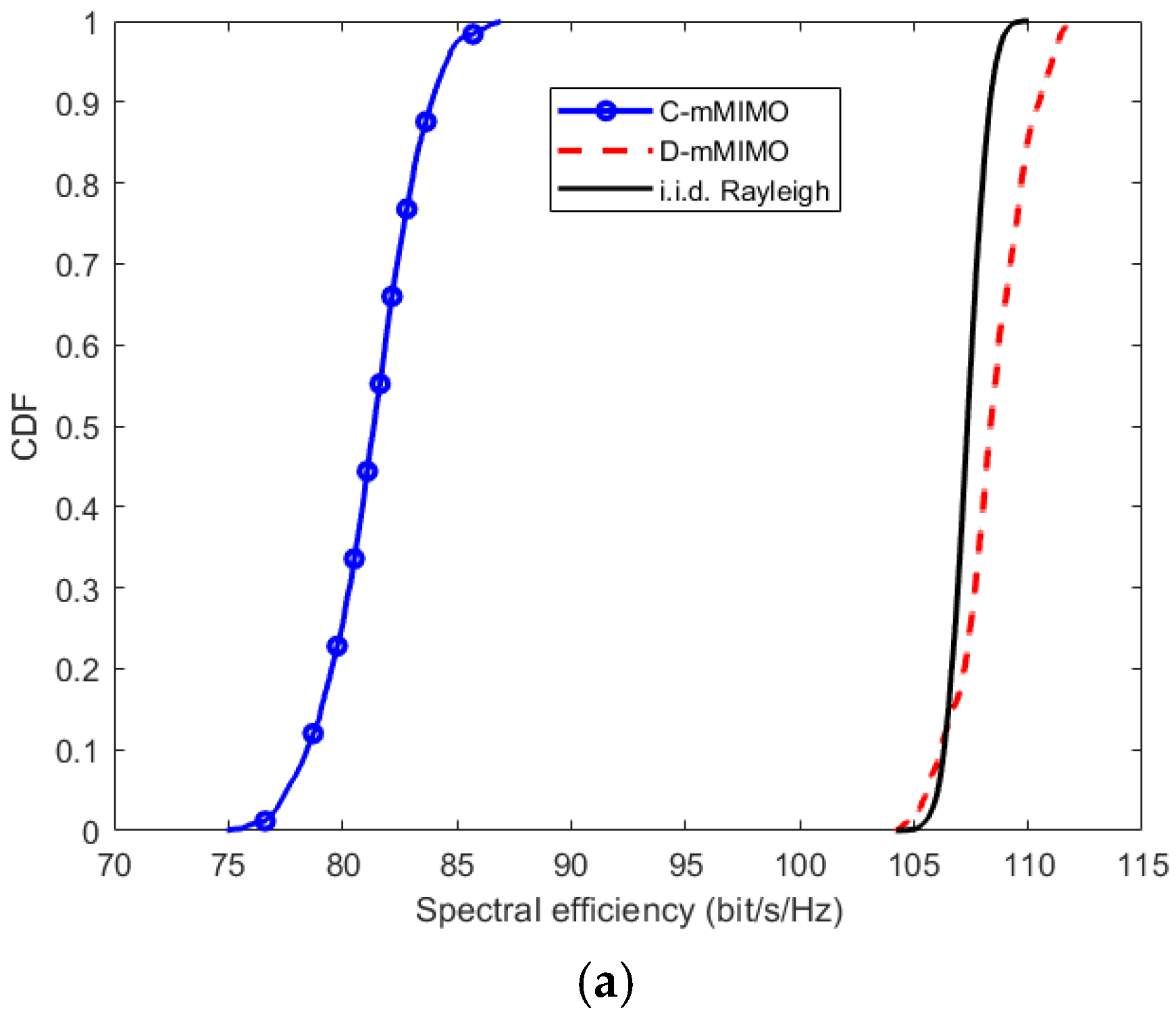
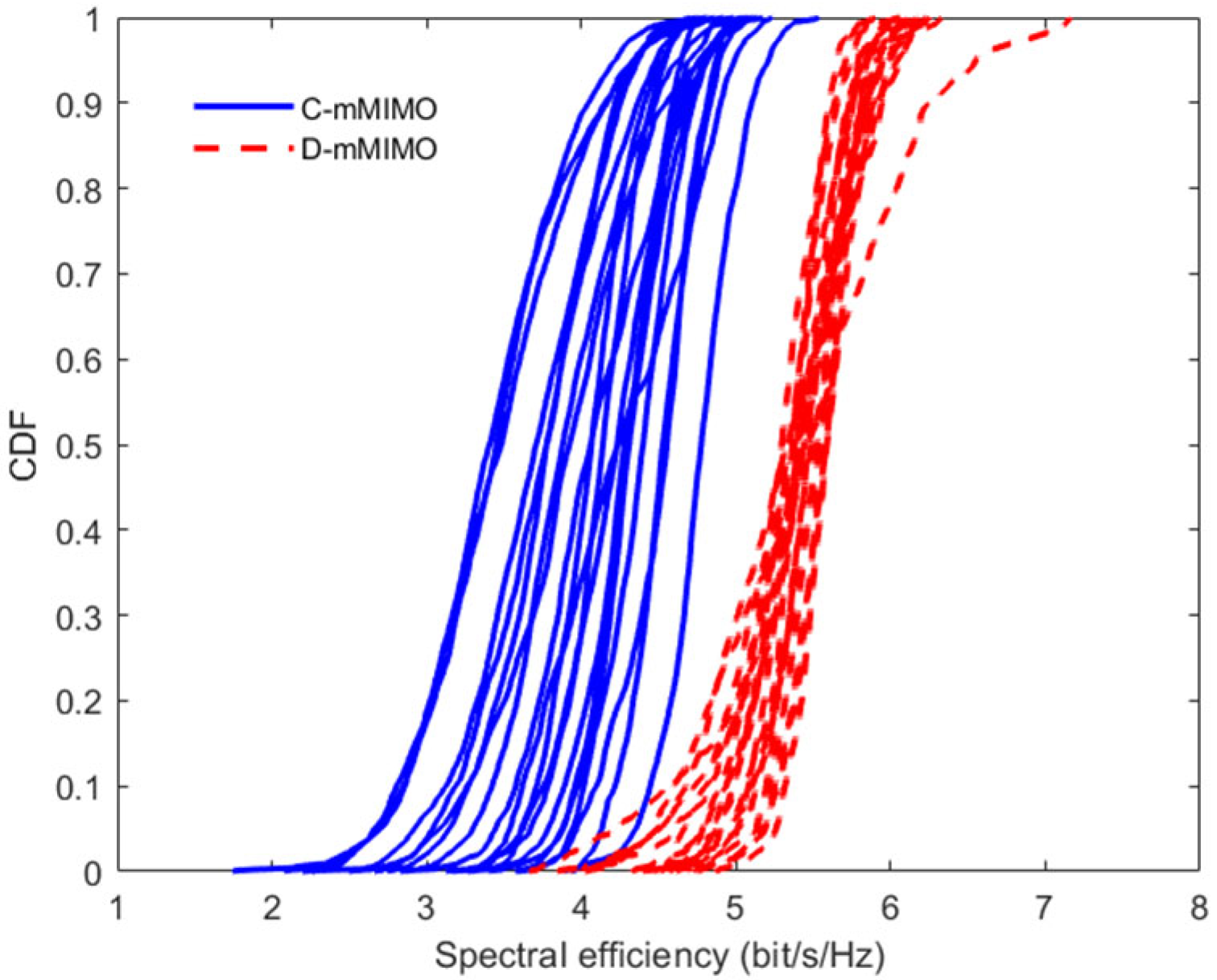
3.2. D-mMIMO Results: Analysis and Discussion

This subsection includes the results achieved with the approach presented in this work for the optimization problem described in the previous subsection.

Figure 7 shows the fitness evolution for the 10 runs of the BPSO algorithm, including the averaged fitness. Analyzing the individual final residual errors obtained, they range from 46.93 (BPSO_best) to 51.53 (BPSO_worst), corresponding to the best and worst solutions achieved for the D-mMIMO system, consisting of 46 and 49 active antennas at the BS, respectively. As stated in Section 2.3, concerning the fitness function proposed in (16), the results obtained show how BPSO focuses on the exploration of the search space during the initial iterations until the errors in both SE and JFI become insignificant and then, it concentrates on trying to reduce as much as possible the number of active antennas, related to the third addend in (16), which has the most influence on the error, i.e., F_p in (16), as the iterations progress. The antenna deployments proposed by the 10 runs range from 46 to 49 of the initial set consisting of 100 locations, a significant reduction that would contribute to saving power and reducing the complexity of the network.

Figure 8 shows the results achieved considering both the best and the worst of the 10 simulations, intentionally compared to show the stability and accuracy of the solutions in terms of SE and JFI, taking as reference the QoS imposed by the C-mMIMO channel. In both Figure 8a,b, the CDF adjustments achieved for the D-mMIMO system exhibit great accuracy in the QoS provided to the 20 UTs, demonstrating the usefulness of the methodology proposed.

Focusing on the best solution (BPSO_best), the optimizer proposes to activate for the D-mMIMO system only 46 of the potential 100 antenna locations, according to the optimized spatial distribution shown in Figure 8c. From the results, it can be observed that the antennas activated are almost uniformly distributed over the environment, as is the case with the 20 UTs considered. With the normalization used in (4), equivalent to an ideal power control, the near–far effect is minimized. Consequently, antennas are selected to increase macrodiversity, which results in orthogonality between the channels of different users and a decrease in the interferences in (7). In addition, the decrease in the number of antennas obtained in the D-mMIMO system results in a reduction in signal processing and an increase in energy efficiency (EE) for the mobile network, contributing also to the reduction in digital carbon footprint.

4. Conclusions

In this work, we have presented an antenna selection approach in a D-mMIMO system which, starting from a maximum of 100 antenna locations, selects and activates those that offer the same QoS as a C-mMIMO system, with an array consisting of 100 antennas taken as reference. In the selection/optimization process, a BPSO algorithm was used, with a cost function to be minimized that takes into account the differences in the sum SE, the JFI fairness factor, and rewards solutions with fewer active receiver antennas. The results obtained in a large indoor environment at 26 GHz show that, for the case study of 20 UTs considered, the number of active antennas in the distributed array is more than halved.

The cost function used can be changed, with the optimal solution not necessarily being the performance of a concentrated array; other values of SE or JFI can be taken into account, determined by the QoS to be provided. Furthermore, it is worth highlighting the significant reduction in power consumption, signal processing, and network traffic achieved by reducing the number of antennas. Although a quantitative analysis of the EE increase is beyond the scope of this work, it seems obvious that a large reduction in the number of receiver antennas necessary to achieve predetermined QoS values clearly influences the EE in the cell.

Finally, two lines of research that the authors consider of interest and on which they are already working are, first, considering new propagation environments with a different number of UTs, and second, carrying out the antenna selection task simultaneously considering both the up-link and the down-link. In the future, the methodology could be applied to more realistic deployments, involving a higher number of UTs in the cell, multicell scenarios, or even its application using AI-based methods as the optimization core to obtain solutions in real time. This would make it possible to improve user scheduling techniques, interacting efficiently with the upper layers of the network.

References

1. Larsson, E.; Edfors, O.; Tufvesson, F.; Marzetta, T. Massive MIMO for next generation wireless systems. IEEE Commun. Mag. 2014, 52, 186–195. [Google Scholar] [CrossRef]
2. Björnson, E.; Sanguinetti, L.; Wymeersch, H.; Hoydis, J.; Marzetta, T.L. Massive MIMO is a reality—What is next?: Five promising research directions for antenna arrays. Digit. Signal Process. 2019, 94, 3–20. [Google Scholar] [CrossRef]
3. Wang, Z.; Zhang, J.; Du, H.; Sha, W.E.I.; Ai, B.; Niyato, D.; Debbah, M. Extremely large-scale MIMO: Fundamentals, challenges, solutions, and future directions. IEEE Wirel. Commun. 2024, 31, 117–124. [Google Scholar] [CrossRef]
4. Ngo, H.Q.; Interdonato, G.; Larsson, E.G.; Caire, G.; Andrews, J.G. Ultradense cell-free massive MIMO for 6G: Technical overview and open questions. Proc. IEEE 2024, 112, 805–831. [Google Scholar] [CrossRef]
5. Zhou, S.; Zhao, M.; Xu, X.; Wang, J.; Yao, Y. Distributed wireless communication system: A new architecture for future public wireless access. IEEE Commun. Mag. 2003, 41, 108–113. [Google Scholar] [CrossRef]
6. Ngo, H.Q.; Ashikhmin, A.; Yang, H.; Larsson, E.G.; Marzetta, T.L. Cell-Free Massive MIMO Versus Small Cells. IEEE Trans. Wirel. Commun. 2017, 16, 1834–1850. [Google Scholar] [CrossRef]
7. Interdonato, G.; Björnson, E.; Quoc, H.; Frenger, P.; Larsson, E.G. Ubiquitous cell-free Massive MIMO communications. J. Wirel. Commun. Netw. 2019, 197, 197. [Google Scholar] [CrossRef]
8. Dai, H. Distributed Versus Co-Located MIMO Systems with Correlated Fading and Shadowing. In Proceedings of the IEEE International Conference on Acoustics Speed and Signal Processing, Toulouse, France, 14–19 May 2006; pp. 561–564. [Google Scholar] [CrossRef]
9. Dai, L. A Comparative Study on Uplink Sum Capacity with Co-Located and Distributed Antennas. IEEE J. Sel. Areas Commun. 2011, 29, 1200–1213. [Google Scholar] [CrossRef]
10. Almelah, H.B.; Hamdi, K.A. Spectral Efficiency of Distributed Large-Scale MIMO Systems with ZF Receivers. IEEE Trans. Veh. Technol. 2017, 66, 4834–4844. [Google Scholar] [CrossRef]
11. Clark, M.V.; Willis, T.M.; Greenstein, L.J.; Rustako, A.J.; Erceg, V.; Roman, R.S. Distributed versus centralized antenna arrays in broadband wireless networks. In Proceedings of the IEEE VTS 53rd Vehicular Technology Conference, Rhodes, Greece, 6–9 May 2001; Volume 1, pp. 33–37. [Google Scholar] [CrossRef]
12. Kumagai, S.; Kobayashi, T.; Oyama, T.; Akiyama, C.; Tsutsui, M.; Jitsukawa, D.; Seyama, T.; Dateki, T.; Seki, H.; Minowa, M.; et al. Experimental trials of 5G ultra high-density distributed antenna systems. In Proceedings of the IEEE 90th Vehicular Technology Conference, Honolulu, HI, USA, 22–25 September 2019; pp. 1–5. [Google Scholar] [CrossRef]
13. Chen, C.; Guevara, A.P.; Pollin, S. Scaling up distributed massive MIMO: Why and how. In Proceedings of the 51st Asilomar Conference on Signals, Systems, and Computers, Pacific Grove, CA, USA, 29 October–1 November 2017; pp. 271–276. [Google Scholar] [CrossRef]
14. Okuyama, T.; Suyama, S.; Mashino, J.; Okumura, Y.; Shiizaki, K.; Akiyama, C. Antenna Deployment of 5G Ultra High-Density Distributed Massive MIMO by Low-SHF-Band Indoor and Outdoor Experiments. In Proceedings of the IEEE 86th Vehicular Technology Conference, Toronto, ON, Canada, 24–27 September 2017; pp. 1–5. [Google Scholar] [CrossRef]
15. Chen, C.-M.; Wang, Q.; Gaber, A.; Guevara, A.P.; Pollin, S. User Scheduling and Antenna Topology in Dense Massive MIMO Networks: An Experimental Study. IEEE Trans. Wirel. Commun. 2020, 19, 6210–6223. [Google Scholar] [CrossRef]
16. Pérez, J.R.; Fernández, Ó.; Valle, L.; Bedoui, A.; Et-tolba, M.; Torres, R.P. Experimental analysis of concentrated versus distributed massive MIMO in an indoor cell at 3.5 GHz. Electronics 2021, 10, 1646. [Google Scholar] [CrossRef]
17. Pérez, J.R.; Valle, L.; Fernández, O.; Torres, R.P.; Rubio, L.; Rodrigo-Peñarrocha, V.M.; Reig, J. A comparison between concentrated and distributed massive MIMO channels at 26 GHz in a large indoor environment using ray-tracing. IEEE Access 2022, 10, 65623–65635. [Google Scholar] [CrossRef]
18. Fernández, O.; Valle, L.; Domingo, M.; Torres, R.P. Flexible Rays. IEEE Veh. Technol. Mag. 2008, 3, 18–27. [Google Scholar] [CrossRef]
19. Moreno, J.; Domingo, M.; Valle, L.; Pérez, J.R.; Torres, R.P.; Basterrechea, J. Design of Indoor WLANs: Combination of a ray-tracing tool with the BPSO method. IEEE Antennas Propag. Mag. 2015, 57, 22–33. [Google Scholar] [CrossRef]
20. Tsai, C.-W.; Cho, H.-H.; Shih, T.K.; Pan, J.-S.; Rodrigues, J.J.P.C. Metaheuristics for the deployment of 5G. IEEE Wirel. Commun. 2015, 22, 40–46. [Google Scholar] [CrossRef]
21. Sapkota, B.; Ghimire, R.; Pujara, P.; Ghimire, S.; Shrestha, U.; Ghimire, R.; Dawadi, B.R.; Joshi, S.R. 5G network deployment planning using metaheuristic approaches. Telecom 2024, 5, 588–608. [Google Scholar] [CrossRef]
22. Alruwaili, M.; Kim, J.; Oluoch, J. Optimizing 5G power allocation with device-to-device communication: A Gale-Shapley algorithm approach. IEEE Access 2024, 12, 30781–30795. [Google Scholar] [CrossRef]
23. Luna, F.; Luque-Baena, R.M.; Martínez, J.; Valenzuela-Valdés, J.F.; Padilla, P. Addressing the 5G cell switch-off problem with a multi-objective cellular genetic algorithm. In Proceedings of the IEEE 5G World Forum (5GWF), Silicon Valley, CA, USA, 9–11 July 2018; pp. 422–426. [Google Scholar] [CrossRef]
24. Wang, R.; Jiang, Y. Distributed optimization of Uplink Cell-Free Massive MIMO Networks. In Proceedings of the IEEE 96th Vehicular Technology Conference (VTC2022-Fall), London, UK, 26–29 September 2022; pp. 1–5. [Google Scholar] [CrossRef]
25. Gao, Y.; Vinck, H.; Kaiser, T. Massive MIMO antenna selection: Switching architectures, capacity bounds, and optimal antenna selection algorithms. IEEE Trans. Signal Process. 2018, 66, 1346–1360. [Google Scholar] [CrossRef]
26. Ouyang, C.; Ou, Z.; Zhang, L.; Yang, H. Optimal Transmit Antenna Selection Algorithm in Massive MIMOME Channels. In Proceedings of the IEEE Wireless Communications and Networking Conference (WCNC), Marrakesh, Morocco, 15–18 April 2019; pp. 1–6. [Google Scholar] [CrossRef]
27. Benmimoune, M.; Driouch, E.; Ajib, W.; Massicotte, D. Novel transmit antenna selection strategy for massive MIMO downlink channel. Wirel. Netw. 2017, 3, 2473–2484. [Google Scholar] [CrossRef]
28. Souza, J.H.I.; Amiri, A.; Abrão, T.; Carvalho, E.; Popovski, P. Quasi-distributed antenna selection for spectral efficiency maximization in subarray switching XL-MIMO systems. IEEE Trans. on Veh. Technol. 2021, 70, 6713–6725. [Google Scholar] [CrossRef]
29. Kennedy, J.; Eberhart, R.C. A discrete binary version of the particle swarm algorithm. In Proceedings of the IEEE International Conference on Systems, Man, and Cybernetics, Computational Cybernetics and Simulation, Orlando, FL, USA, 12–15 October 1997; pp. 4104–4108. [Google Scholar] [CrossRef]
30. Khanesar, M.A.; Teshnehlab, M.; Shoorehdeli, M.A. A novel binary particle swarm optimization. In Proceedings of the Mediterranean Conference on Control & Automation, Athens, Greece, 27–29 June 2007; pp. 1–6. [Google Scholar] [CrossRef]
31. Gao, X.; Edfors, O.; Rusek, F.; Tufvesson, F. Massive MIMO Performance Evaluation Based on Measured Propagation Data. IEEE Trans. Wirel. Commun. 2015, 14, 3899–3911. [Google Scholar] [CrossRef]
32. Pérez, J.R.; Torres, R.P.; Domingo, M.; Valle, L.; Basterrechea, J. Analysis of massive MIMO performance in an indoor picocell with high number of users. IEEE Access 2020, 8, 107025–107034. [Google Scholar] [CrossRef]
33. Jain, R.K.; Chiu, D.-M.W.; Hawe, W.R. A Quantitative Measure of Fairness and Discrimination; Eastern Research Laboratory, Digital Equipment Corporation: Hudson, MA, USA, 1984. [Google Scholar]
34. Kennedy, J.; Eberhart, R.C. Particle swarm optimization. In Proceedings of the IEEE International Conference on Neural Networks, Perth, WA, Australia, 27 November–1 December 1995; pp. 1942–1948. [Google Scholar] [CrossRef]
35. ITU. Effects of Building Materials and Structures on Radiowave Propagation Above About 100 MHz; ITU Radiowave Propagation Series Recommendation ITU-R P.2040-3, Release 3; International Telecommunication Union: Geneva, Switzerland, 2023. [Google Scholar]
36. Kennedy, J.; Eberhart, R.C.; Shi, Y. Swarm Intelligence; Morgan Kaufmann: San Francisco, CA, USA, 2001; pp. 289–296. [Google Scholar]
Figure 1. Illustration of mMIMO systems. (a) C-mMIMO cell with Q active users and M antennas at the BS; (b) D-mMIMO system with Q users, in which M distributed BSs are jointly serving the UTs.
Electronics 14 01233 g001
Figure 2. Flowchart of the methodology proposed.
Electronics 14 01233 g002
Figure 3. Top view of the environment (183 × 50 m in size), including locations for both UTs and arrays for C-mMIMO and D-mMIMO systems.
Electronics 14 01233 g003
Figure 4. Analysis of the site chosen for the BS of the C-mMIMO system considered as reference.
Electronics 14 01233 g004
Figure 5. C-mMIMO and D-mMIMO up-link channel results for 20 UTs and 100 receiver antennas. (a) CDF of the sum SE; (b) CDF of JFI.
Electronics 14 01233 g005aElectronics 14 01233 g005b
Figure 6. CDFs of the SE associated with each one of the 20 UTs in both mMIMO systems.
Electronics 14 01233 g006
Figure 7. Fitness evolution for 10 independent runs of the BPSO algorithm.
Electronics 14 01233 g007
Figure 8. D-mMIMO antenna selection results. (a) CDF of the sum SE; (b) CDF of JFI; (c) BPSO best solution with details of the locations of the 46 active antennas.
Electronics 14 01233 g008