Abstract
Security issues surrounding deep learning models weaken their application effectiveness in various fields. Studying attacks against deep learning models contributes to evaluating their security and improving it in a targeted manner. Among the methods used for this purpose, adversarial example generation methods for deep learning models have become a hot topic in academic research. To overcome problems such as extensive network access, high attack costs, and limited universality in generating adversarial examples, this paper proposes a generic algorithm for adversarial example generation based on improved DE-C&W. The algorithm employs an improved differential evolution (DE) algorithm to conduct a global search of the original examples, searching for vulnerable sensitive points susceptible to being attacked. Then, random perturbations are added to these sensitive points to obtain adversarial examples, which are used as the initial input of C&W attack. The loss functions of the C&W attack algorithm are constructed based on these initial input examples, and the loss function is further optimized using the Adaptive Moment Estimation (Adam) algorithm to obtain the optimal perturbation vector. The experimental results demonstrate that the algorithm not only ensures that the generated adversarial examples achieve a higher success rate of attacks, but also exhibits better transferability while reducing the average number of queries and lowering attack costs.
1. Introduction
Deep learning technology is now advancing rapidly in many fields. With the continuous promotion and popularization of deep learning technology, deep learning models have become targets of attacks, and their security has gradually become an obstacle to the future development and application of deep learning technology [1,2,3]. Common security threats in the field of deep learning mainly include data poisoning, backdoor attacks, adversarial example attacks, etc. In particular, the presence of adversarial examples poses a great threat to the security of deep learning networks, which greatly restricts the further development of deep learning applications.
In 2013, Szegedy et al. revealed the fragility of deep neural networks by adding imperceptible perturbations and found that adding a small amount of noise to clean examples correctly classified by the deep neural network produces new images that appear almost identical to the original image to the human eye [4]. After the examples with noise are input into the model again, incorrect prediction results are obtained. These modified examples are called adversarial examples. The concept of adversarial examples was proposed by Goodfellow et al. in 2014, referring to the input examples formed by adding small perturbations that are difficult to detect by human vision to the original examples [5]. Adversarial examples can be used to deceive deep learning systems, causing them to make incorrect decisions or classifications. To better evaluate the security of deep learning models and identify targeted methods to defend them against adversarial example attacks, it is necessary to study effective high-performance adversarial example generation methods.
The main work conducted in this paper is described as follows:
- A generic algorithm for adversarial example generation based on DE-C&W is proposed, which uses the DE algorithm to preprocess the data and the Adam algorithm to optimize the loss function of C&W to improve the universality and success rate of adversarial example attacks;
- The improved DE algorithm is used to preprocess the initial examples to reduce the initial search dimension of the C&W algorithm and improve the accuracy of searching for effective attack points, enhancing the query efficiency while ensuring the success rate of the attack;
- The scaling factor is adaptively adjusted based on the two individuals that generate the differential vector, and the fitness function is used to adaptively control the change in the crossover probability factor of the DE algorithm, improving the global optimization ability and accelerating the convergence rate. Through the introduction of a new mutation strategy that balances global search and local development capabilities, the accuracy of searching for effective attack points is improved, and the effectiveness and efficiency of adversarial example attacks are enhanced;
- The loss function of C&W is redefined and its gradient calculation method is improved, making it possible to implement black-box attacks by obtaining only the probability value of the model label, thereby improving the portability of the adversarial examples. The loss function is further optimized by using the Adam optimization algorithm, which is less affected by local minima and has a faster convergence speed, to find the optimal perturbation and improve the speed of finding the optimal solution;
- The comparative experimental results show that the algorithm reduces the average number of queries and attack cost while ensuring the success rate of adversarial example attacks;
Next, work relevant to this paper will be introduced, followed by an adversarial example generation algorithm based on improved DE and C&W. Finally, the effectiveness of the algorithm will be verified through comparative experiments.
2. Related Work
The emergence of adversarial examples poses a great threat to the security of deep learning models itself and brings new challenges to the security and stability of deep learning systems. Since the concept of adversarial examples was proposed, more and more adversarial attack methods have been introduced, and the security of deep learning systems is increasingly threatened [6,7,8].
At present, adversarial example attacks on deep learning can be roughly divided into two categories: white-box attacks and black-box attacks. Among these, a white-box attack refers to an attack carried out by an attacker who knows all the information, such as the training set, type, structure, and parameters, of the target model. Black-box attacks are completely opposite to white-box attacks, as attackers have no internal information about the target model and can only carry out attacks by observing the input and output of the model.
A white-box attack is an ideal attack scenario that can be used to evaluate the security threshold of deep learning models. White-box attacks pose a significant threat to the model due to the attacker’s complete understanding of the internal information of the model, which allows for more accurate and effective modification or destruction of the model’s prediction results. Goodfellow et al. proposed the Faster Gradient Sign Method (FGSM) [5], which adds a specific perturbation value to each pixel of the input data to misclassify the perturbed data. This algorithm is easy to implement and has a high success rate. In subsequent research on adversarial attacks, it has not only been widely used but also become a benchmark method for evaluating algorithm performance and efficiency. The Basic Iterative Method (BIM) attack algorithm proposed by Kurakin et al. is an iterative adversarial attack method that adds small perturbations to the original input examples through multiple iterations, gradually increasing the addition of perturbations to the original input examples, and recalculating the gradient direction after each iteration to construct more accurate perturbations [9]. The DeepFool attack algorithm proposed by Moosavi et al. is a novel white-box attack method based on iterative thinking. It does not limit the range of original example perturbations and can generate smaller perturbations than fast gradient attacks [10]. However, this algorithm can only deceive a single deep learning model, and the perturbation size needs to be manually set, requiring a lot of prior knowledge. In 2021, Xiao et al. first proposed the Adversarial Generative Adversarial Network (AdvGAN) attack, which utilizes the adversarial training of generators and discriminators to transform random noise into aggressive adversarial examples [11].
Compared to white-box attacks, black-box attacks require less prior knowledge and are more difficult to implement. Researchers have proposed many typical black-box attack algorithms. Brendel et al. proposed the boundary attack algorithm, which is a decision-based attack method that attacks the classification results of the attacked classifier [12]. This algorithm performs well in terms of adversarial example generation efficiency, but requires a large amount of computation, resulting in high costs of time and computation. Chen et al. proposed the Zeroth Order Optimization (ZOO) algorithm attack, which is similar to the C&W attack in terms of optimization methods, with both using the optimizing loss function to generate adversarial examples [13,14]. Unlike C&W attacks, ZOO is a method that only accesses the input and output of the model, allowing for model optimization without solving gradients, and has wide applicability. Tu et al. proposed an autoencoder-based Zeroth Order Optimization method (Autozoom) to solve black-box optimization problems [15]. This method models the objective function through an autoencoder and then optimizes it using the intermediate features obtained from the modeling. Su et al. proposed the One Pixel Attack algorithm, which can implement attacks by modifying only one pixel in an image [16].
Black-box attacks can only rely on simple input and output mapping information to attack unknown models, which leads to low success rates and a high number of queries. At present, the success rate and query count are still the most fundamental issues of concern for scholars regarding black-box attacks. To reduce the number of queries to the target model in adversarial attacks, Da et al. proposed a gradient-free adversarial attack algorithm based on differential evolution [17]. Two fitness functions were designed to implement targeted and non-targeted attacks, and an elimination mechanism was introduced in the selection stage to accelerate the convergence of the algorithm. To solve the problem of the low success rate of black-box attacks in adversarial example attacks, Xie et al. combined basic iterative algorithms and momentum iterative algorithms with other attack methods and increased the diversity of attack methods to improve the success rate of attacks [18]. Huang Lifeng et al. proposed an attack method based on a covariance matrix and adaptive evolution strategy to reduce the number of interactive queries and improve attack efficiency [19]. Hu et al. proposed a MalGAN algorithm based on Generative Adversarial Networks (GANs) to generate adversarial malicious examples, which can reduce the model detection rate to near zero and make it difficult for retraining-based adversarial example defense methods to work [20]. Yang et al. introduced the AdaBelief optimizer and crop invariance in the generation of adversarial examples, and proposed the AdaBelief Iterative Fast Gradient Method (ABI-FGM) and Crop Invariant Attack Method (CIM), to improve the transferability and attack success rate of adversarial examples [21]. These studies demonstrate new advances in the field of adversarial attacks, particularly in improving attack efficiency, reducing detection rates, and enhancing the imperceptibility and transferability of adversarial examples. The development of these methods is of great significance for understanding and defending against potential adversarial attacks.
Black-box adversarial example attacks generally have low universality, have low efficiency in generating adversarial examples, and require repeated access to the attacked network. In practical applications, this not only results in high attack costs but is also easily detected by the other party. This article proposes a general adversarial example generation algorithm based on improved differential evolution to address these issues. This algorithm uses an improved differential evolution algorithm to preprocess the input image, finding multiple sensitive pixels that are easily attacked, reducing the number of queries and lowering attack costs. Then, through the use of backpropagation, the adversarial attack problem is transformed into an optimization problem, and the problem of generating adversarial examples is redefined as an unconstrained optimization problem. Afterward, the loss function in the C&W attack algorithm is reconstructed so that it does not require the obtaining of internal parameter information of the deep neural network. Then, the Adam optimization algorithm is used to optimize the loss function to accelerate convergence, search for the optimal solution, that is, the minimum perturbation, and minimize the difference between the adversarial example and the original example when the deep learning model identifies errors.
Table 1 compares the adversarial example attack methods mentioned above with the method proposed in this paper in terms of accuracy (or advantages), query frequency, and limitations.

Table 1.
Comparison of different adversarial example attack methods.
3. Adversarial Example Generation Based on DE-C&W
C&W is an optimization-based adversarial attack generation algorithm, classified as a white-box attack algorithm [14]. It can dynamically adjust confidence and strike a balance between attack accuracy and adversarial perturbation, thereby achieving true adversarial sample generation effects. Although this attack can evade many defense methods, due to its optimization-based approach, parameter updates require a significant amount of time, resulting in a longer time needed to generate adversarial samples, which is not as fast as other attack methods. Therefore, C&W is rarely used to generate adversarial examples in Artificial Intelligence (AI) adversarial example competitions. In response to the slow and time-consuming generation of C&W adversarial examples, this paper first uses the differential evolution (DE) algorithm to preprocess the input examples to reduce the number of queries and search dimensions. Then, the Adam optimization algorithm is used to avoid the impact of gradient scaling on parameter updates, so as to achieve the optimization goal of faster convergence speed.
3.1. Optimization of C&W Attack
In 2017, Carlini and Wagner proposed an optimized C&W attack algorithm to attack defensive distillation networks [14]. This algorithm uses the following optimization formula to obtain the initial adversarial examples:
In Formulas (1) and (2), represents the adversarial example, represents the initial input example, and represents the adversarial perturbation added to the initial input example. represents the distance metric between the original example and the adversarial example , usually using the Euclidean distance metric. c is an optional constant used to balance the relationship between two loss functions, where the larger the value of c, the higher the success rate of the attack, and the longer the time taken; P represents the dimension, represents a P-dimensional hypercube, and the values of each dimension in are in the range of [0, 1]. represents the loss function of the deep learning model, the function refers to the i-th output of the previous layer of softmax in the deep neural network model, i represents the category of the original input data, t is the category judged as incorrect, and parameter k is used to constrain the minimum value of confidence.
The C&W attack first uses the loss function to replace the predicted output of the deep model for adversarial samples if and only if ≤ 0. Then, the Lagrange rule is used to transform the predicted output class of the deep model for adversarial samples into the optimization problem shown in Formula (1). This attack algorithm has made various attempts to modify the loss function, using as a distance measurement scale to explore multiple custom loss functions, in order to find the loss function with the best attack effect, as shown in Formula (2). Using this loss function only requires the confidence of a misclassified category t to exceed the confidence of the original category i. At the same time, the algorithm uses Formula (3) to impose box constraints on adversarial sample An, transforming the problem of optimizing adversarial example into the problem of optimizing independent variable w.
where w is the independent variable in tanh space, representing the optimized parameter. After the mapping transformation of the formula, the perturbation is obtained. This method ensures that the generated adversarial samples, regardless of how the parameter w is adjusted, will not exceed the normal range of the data after mapping transformation, thus transforming the box-constrained optimization problem into an unconstrained optimization problem, which is convenient for the subsequently used optimizers to solve.
In the improved C&W attack algorithm, the loss function does not need to obtain detailed parameter information of the deep neural network, but needs to transform the adversarial attack problem into an optimization problem through backpropagation. Therefore, this algorithm makes the loss function related only to the output results and classification labels of Z (.), and independent of the detailed parameter information of the deep neural network. The improved attack algorithm is shown in Formula (4).
In this formula, represents the modified loss function, represents the range of values that restrict the addition of perturbations, and represents the predicted output of the deep model for adversarial examples. The reason for the existence of upper and lower bounds is that the range of pixel values that digital images can represent is limited. After normalization, pixel values are constrained within the range of [0, 1]. In order to ensure the effectiveness of the image after perturbations are added, a new variable w is introduced in Formula (3) to limit the range of perturbation values in the experiment. Since the range of the tanh function itself is [−1, 1], this ensures that the range of An is [0, 1]. In addition, since the limitation of pixel values relies on the range of the loss function itself rather than artificial truncation, some optimizers that do not support artificial truncation can be introduced, such as the Adam optimization method. The modified loss function does not require the obtaining of detailed parameter information of the deep neural network. At the same time, the output of the neural network is converted to log(.) and monotonically transformed, which can better represent the probability distribution and clarify the confidence of each category. The adjusted loss function is shown in Formula (5).
In the optimized attack, when An is judged as a class other than the original label i, it indicates that the generated adversarial example attack has been successful.
3.2. Adam Optimization Algorithm
Liu et al. used a finite-difference-based method in the FGSM to estimate the gradient of the model for a certain input example when solving the adversarial example attacks [22]. The FGSM attack method generates adversarial examples quickly and only needs the gradient information of the model output to be calculated once, but the quality of the generated adversarial examples is low. Another query can provide second-order information. The formula is as follows:
where x indicates a certain attacked pixel of an input example; indicates a function of the target model; indicates the value of the j-th dimension of the attacked pixel; indicates the gradient value of the j-th dimension of the deep learning model for a certain input example x; and indicates the second-order gradient value of the j-th dimension of the deep learning model for a certain input example x. h indicates a sufficiently small number; is the unit vector of the j-th dimension. The algorithm adjusts the calculation accuracy and efficiency of the gradient around the estimated pixel by adjusting the small variation h. The method is suitable for large-scale deep neural networks and can effectively deal with adversarial attacks, but it may lead to a large number of model queries, thereby reducing query efficiency. Therefore, gradient estimation methods have received increasing attention from scholars in recent years.
The Adam algorithm was proposed by Kingma and Lei in 2014 [23]. Subsequently, it became very popular in the field of deep learning because it can quickly achieve excellent results with high computational efficiency, convenient implementation, and minimal memory usage. The improved C&W attack algorithm cannot directly obtain the gradient information of the target model. Through the construction of an optimization problem, the attack target is transformed into a problem of minimizing the loss function, and the input image is used as the initial point to search for the optimal solution. During the search process, the algorithm utilizes the gradient information estimated through output results and classification labels as the search direction to find the optimal solution. The Adam algorithm is different from traditional stochastic gradient descent methods. The traditional stochastic gradient descent method uses a single learning rate to update all weights and searches for the optimal solution with the estimated gradient as the initial direction. In contrast, the Adam algorithm combines the ideas of the momentum method and adaptive learning rate, and designs independent adaptive learning rates for different parameters by calculating the first-order moment estimate (i.e., the mean of the gradients) and second-order moment estimate (i.e., the uncentered variance of the gradients) of the gradient [24,25]. For the t-th time step, the first-order moment estimate and second-order moment estimate of the gradient can be calculated separately according to the following formulas:
where indicates the first-order moment estimate of the model gradient at moment t, indicates the second-order moment estimate of the model gradient at moment t, indicates the first-order moment estimate of the model gradient at moment , indicates the second-order moment estimate of the model gradient at moment , indicates the gradient of the redefined loss function, and and are the decay rates of the two exponentially weighted averages, respectively. The Adam algorithm is simple and easy to implement, with high computational efficiency and low memory requirements. Its parameter updates are not affected by the learning rate adjustment problem caused by gradient scaling transformation, so it can converge faster and find the optimal solution faster than the traditional stochastic gradient descent method.
3.3. Differential Evolution Algorithm
In order to find optimal solutions in multidimensional spaces, Price and Storn [26] developed a straightforward yet effective population-based global optimization evolutionary algorithm known as differential evolution (DE). Because of its straightforward structure, simple implementation, quick convergence, and robustness, it is widely utilized. At the first international contest on evolutionary optimization (ICEO) held in Nagoya, Japan, in 1996, the differential evolution algorithm proved to be the fastest evolutionary algorithm.
The differential evolution algorithm generates population individuals by using floating-point vector encoding. In the optimization process of the differential evolution algorithm, firstly, two individual vectors are randomly selected from the parent individual vectors to generate the difference vector, and then another individual vector is selected and added to the differential vector to obtain the experimental individual. For the convenience of pixel localization and to meet the requirement that the input values of the differential evolution algorithm are vectors, a pixel is represented as a five-tuple p = (x, y, r, g, b), where x, y represents the coordinates of the pixel, and r, g, and b denote the red, green, and blue color channel values of the pixel. When perturbations are added, the same vector form is employed for presentation, and the perturbation values are added to the corresponding r, g, and b channels of the pixel, with each mutant containing a fixed number of perturbed vectors. The mutation formula is as follows:
where is the mutant individual corresponding to the target individual , that is, the i-th mutant in the population of the (G + 1)-th generation; r1, r2, and r3 are three randomly selected integers from the parent generation that are different from i; , , and are three mutually different individuals randomly selected from the current g-th generation population and are different from the target individual ; and F is the scaling factor, which generally ranges from 0 to 1.
Through the use of the crossover formula indicated below, the parent individuals are crossed with the corresponding experimental individuals to generate new offspring individuals.
where rand(0, 1) yields a random number in the range of (0, 1); CR is the crossover control parameter; is a random component that ensures that an at least one-dimensional component is provided by the mutant individuals after the crossover; indicates the value of mutant individual i in the (G + 1)-th generation population in the j-th dimension (or component j); indicates the value of individual i in the G-th generation population in the j-th dimension, that is, the value of target individual on component j; and indicates the value of the i-th new individual in the (G + 1)-th generation population generated by the final crossover on component j.
Ultimately, a selection operation is carried out between the parent and offspring populations, and the individuals who satisfy the criteria are saved for the population of the following generation. The formula is as follows:
where indicates the i-th mutant selected from the (G + 1)-th generation population; indicates the i-th mutant in the (G + 1)-th generation population; indicates the target individual, that is, the i-th individual in the G-th generation population; and is the problem to be optimized. Formula (12) is used to compare the cross vector with the original vector and choose the better one, that is, decide which is better, or .
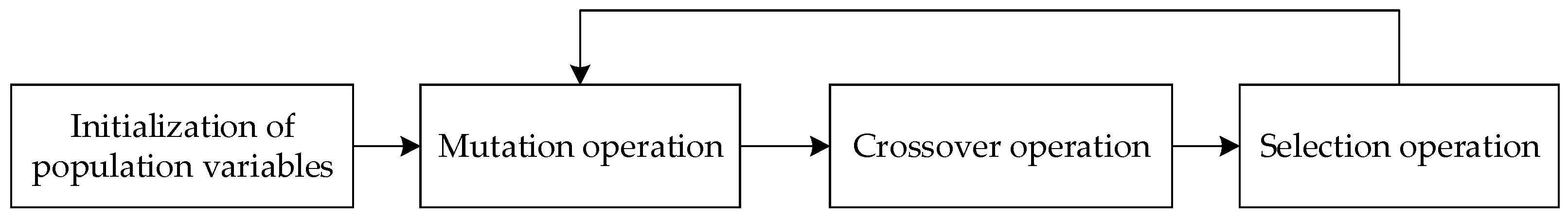
Figure 1 depicts the differential evolution algorithm’s iterative flow.
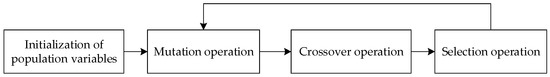
Figure 1.
The iterative flow of the differential evolution algorithm.
While images are preprocessed, the differential evolution algorithm is used to both detect the pixels that are vulnerable to attack and minimize the dimensionality of the query to increase its efficiency. Using the information of direction and distance between vectors or individuals in the population is the essence of DE, as can be seen above in the method of selecting the best option. The Adam optimization algorithm is applied to the search for perturbation points in images. The pixels in the image are the experimental individuals, and the image is used as the input vector. After the differential evolution algorithm’s mutation, crossover, and selection operations, the pixels that have the biggest effects on the deep learning model after being perturbated are searched, and then pixels within a small neighborhood are searched with these pixels as the center, reducing the query dimension of the optimization algorithm.
3.4. Improved Differential Evolution Algorithm
The population size NP, scaling factor F, and crossover probability CR play a crucial role in the execution of the differential evolution algorithm, which can affect the global search capability and local search accuracy of the algorithm. The population size NP determines the parallelism of the algorithm and the breadth of the search space, the scaling factor F determines the degree of individual variation and the depth of the search space, and the crossover probability CR determines the degree of individual crossover and the locality of the search space. Therefore, in the application of the differential evolution algorithm, it is necessary to set and adjust the parameters reasonably to obtain the optimal search performance. The optimal setting of control parameters has different requirements for time consumption and accuracy for different problems. In this paper, the improvement of the differential evolution algorithm mainly focuses on three aspects, namely, the parameter scaling factor F, crossover probability CR, and adjustment of the mutation strategy.
- Optimization of scaling factor F
In traditional differential evolution algorithms, the scaling factor F and crossover probability CR are usually set to fixed values, which often limits the global and local search capabilities of the algorithm [27]. The general range of values for F is between 0 and 1, and the upper limit of 1 is only based on experience and does not mean that there are no successful optimization cases when the value of F is greater than 1. The lower limit of 0 is only a reasonable value recognized by experience. Even in the range of 0 to 1, in some cases, values of the scaling factor F that are almost the same can have a significant impact on the results. The three individuals randomly selected in the mutation operation are sorted according to their fitness and identified, from best to worst, as Xb, Xm, and Xw, and their corresponding fitness values are fb, fm, and fw. The mutation operator is calculated according to the following formula:
In the search space, when the distance between the two individuals Xm and Xw that generate the differential vector is short, that is, when the value of the differential vector (Xm − Xw) is small, in order for the evolutionary algorithm to have a good global search ability in the early stages of evolution, a larger F value should be taken. On the contrary, a smaller F value should be taken to limit larger perturbations and ensure better local search capabilities [28,29,30]. Therefore, this paper adaptively adjusts the value of the scaling factor F based on the fitness of the two individuals generating the differential vector, in order to achieve a balance between global search capability and local search capability, as shown in Formula (14).
In this formula, Fmin = 0.1 and Fmax = 0.9 are set as the minimum and maximum values of the scaling factor [28,29,30,31].
- Optimization of crossover probability CR
In the differential evolution algorithm, the parameter CR controls the degree of the crossover operation. A larger CR value can improve the diversity and search speed of the algorithm, but it may also lead to the algorithm getting stuck in local optimal solutions; a smaller CR value can avoid the premature convergence of the algorithm, but it may also lead to limitations in the search space. According to the crossover formula, the crossover probability CR is used to control the proportion of mutated individuals in the population. A larger CR value is beneficial for increasing individual variability and maintaining population diversity, accelerating local convergence ability, but may lead to premature convergence [30]. In the later stages of the evolutionary process, smaller CR values should be set to drive poorer individuals to evolve toward the global optimum and escape from local optima. Therefore, the fitness function can be used to adaptively control the variation in the crossover probability CR, as shown in Formula (15).
In this formula, CRmax and CRmin are the upper and lower limits of two pre-set crossover probabilities, taken as 0.5 and 0.1, respectively [32]. When the CR value is adaptively adjusted, the range of CR values is limited to [CRmin, CRmax] to ensure that the CR value is not too large or too small; fi is the fitness value of individual Xi; fmax is the optimal fitness value for individuals in the population, while fmin is the worst fitness value for individuals in the population; and represents the average fitness of the current population.
- Improvement in mutation strategy
The mutation strategy is one of the core steps of the differential evolution algorithm, which determines the performance of the algorithm in global and local optimization, and different mutation strategies may also have a great impact on search results [33,34,35]. Therefore, the selection and design of mutation strategies are of great significance for enchancing the performance t and expanding the application of differential evolution algorithms. Formula (10) is also the most commonly used mutation strategy, which is a free-search evolutionary mode that is beneficial for maintaining population diversity. However, in the later stages of the search, it often falls into local optima, resulting in a significant decrease in convergence speed and a tendency for premature convergence [36,37]. Therefore, inspired by the above strategies, this paper adopts a new mutation strategy that can balance global search and local development capabilities, as shown in Formula (16).
In this formula, represents the value of offspring individual at this gene locus, G represents the current generation, (G + 1) represents the next generation, , , and represent the values of three parent individuals at this gene locus, and F is the scaling factor. Due to the linear decreasing trend of scaling factor F, (1 − F) shows a linear increasing trend. According to Equation (16), it can be seen that in the initial stage of optimization, the amplitude coefficient of the base vector is small, and the amplitude coefficients of the differential vectors () are large. However, in the later stage of optimization, the amplitude coefficient of the base vector is large, and the amplitude coefficients of the differential vectors () are small. This strategy can balance population diversity in the early stages of evolution, and in the later stages of the algorithm, it can jump out of local optima and turn to searching for global optima, thereby accelerating convergence speed while also balancing global search capability and local development capability.
3.5. A Generic Algorithm for Adversarial Example Generation Based on DE-C&W
Based on the above-mentioned ideas, this paper proposes a generic algorithm for adversarial example generation based on DE-C&W with the steps outlined below. The algorithm framework is shown in Figure 2.
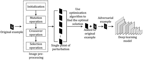
Figure 2.
Flow chart of algorithm framework.
Step 1. Preprocess the original example. Initialize the population and set the crossover control parameter CR, the scaling factor of the difference vector F, the iteration parameter t, and other relevant parameters. Randomly generate N individuals as perturbation vectors, with every perturbation vector being composed of the pixel values and the coordinates of the pixels in the image.
Step 2. Perform the mutation operation. The mutation process of the differential evolution algorithm is carried out in accordance with Formula (16), and the mutations result in new individuals, that is, new perturbation vectors. Each mutated new individual is generated by randomly selecting three individuals from the previous generation and combining them with each other to form the next generation of individuals.
Step 3. Perform the crossover operation. The crossover process of the differential evolution algorithm is performed according to Formula (11), the crossover formula, to obtain a new vector space solution. According to the fitness function value of the optimal individual in the population, dynamically adjust the crossover parameters according to Formula (15), and cross the mutated offspring individuals with the parent individuals to generate a certain number of new individuals.
Step 4. Perform the selection operation. The selection process of the differential evolution algorithm is executed according to Formula (12), and individuals that meet the requirements are selected according to greedy rules to enter the following generation.
Step 5. The iteration ends if the end condition is met; otherwise, steps 2, 3, and 4 are repeated. The end conditions include the number of algorithm iterations reaching a predetermined maximum, the fitness function value converging, or the fitness function value of individuals in the population reaching a predetermined target value.
Step 6. Obtain new input. The random perturbations found are added to the original examples, and the perturbated examples are used as the initial input.
Step 7. Calculate the redefined loss function. Perturbated examples are input into Formula (4), and changes in the output are observed. The loss function is calculated using Formula (5).
Step 8. Estimate the gradient of the loss function. According to Formula (6), the gradient of the loss function is estimated, and the estimated gradient is used as the initial search direction. The Adam optimization algorithm is used to find the optimal solution, which is the optimal perturbation vector.
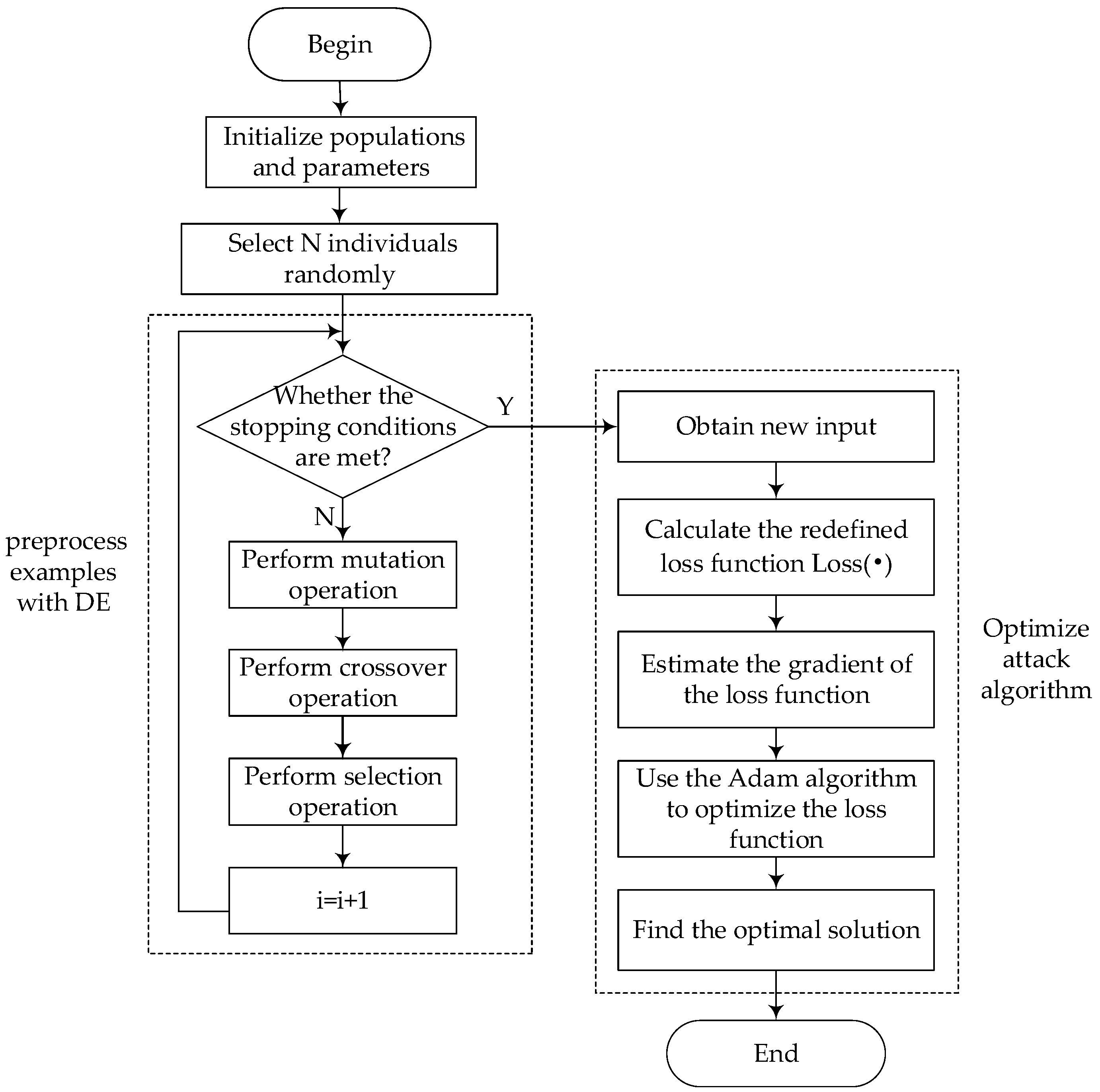
The flow of this adversarial example generation algorithm is shown in Figure 3. The algorithm improves the C&W attack algorithm by modifying the loss function, making it rely only on the output of and the classification label, thereby transforming the attack objective into solving the problem of minimizing the loss function. An improved Adam optimization algorithm is used to determine the optimal perturbation when the attacker is unable to grasp the loss function of the network to be attacked and its gradient, and the difference between the attack image and the original image is minimized when the deep learning model makes a recognition mistake.

Figure 3.
Flow chart of the generic adversarial example generation algorithm based on optimized DE-C&W.
4. Experiments and Analysis of Results
4.1. Experimental Environment
This experiment uses classic ZOO and One Pixel algorithms and the adversarial example generation algorithm proposed in this paper to attack three deep models—LeNet, ResNet, and a custom deep learning model, and compares the performance of the three algorithms in terms of the attack success rate, average attack time, and average number of queries. The experiment was conducted on a computer with 16GB of RAM, a GTX_1650 GPU, and an AMD R5 5600H 3.3 GHz CPU; the operation system is Windows 11, the programming language used is Python 3.10.1, and the equipped deep learning frameworks are Pytorch 1.8.1, Tensorflow 2.6.0, and Keras 2.6.0.
The deep learning model used in this paper is trained on the MNIST and Cifar-10 datasets. The dataset is split into two parts: a training set and a testing set. The CIFAR-10 dataset is a 32 × 32 × 3 color image dataset containing 10 categories, namely, airplane, automobile, bird, cat, deer, dog, frog, horse, ship, and truck. This dataset is a classic dataset used for image classification, where classifications are independent of each other and do not overlap. In the dataset, there are 50,000 training sets and 10,000 testing sets.
The MNIST dataset is a handwritten digit dataset containing 70,000 grayscale images of size 28 × 28, with 10 classifications ranging from 0 to 9. The training set consists of 60,000 images and labels, while the test set consists of 10,000 images and labels. The training set is used to train the network, while the test set is used to construct adversarial examples, but only correctly recognized images are used to generate adversarial examples.
4.2. Experimental Parameter Settings
Because the number of input channels in the two datasets is different, the structure of the deep learning model also needs to be adjusted accordingly. To solve this problem, the experiment draws on the idea of transfer learning. Firstly, a deep learning model is designed based on a dataset, and then the structure of the model is reused by adding a new input layer in front of it as a deep learning model for classifying another dataset. For example, the deep learning model for the CIFAR-10 dataset has an input layer size of 32 × 32 and 3 channels. So, for the deep learning model of MNIST, the same network structure can be used, but a new layer with a size of 28 × 28 and a channel count of 1 can be added before its input layer as the new input layer, and the output of this layer can be adjusted to a size of 32 × 32 and a channel count of 3 to adapt to the input layer size and channel count of the CIFAR-10 dataset. The structure of the LeNet deep learning model trained on the datasets CIFAR-10 and MNIST is shown in Table 2.
Table 2.
The network structure and parameters of the LeNet model.
For higher classification accuracy, the residual network model ResNet50 was chosen [38]. The model first performs feature extraction on the input image through a convolutional layer, followed by pooling operation to reduce the size of the feature images. Then, a series of residual structures is used so that the model can learn and extract the feature images. Finally, the model undergoes average pooling sampling operation and fully connected layer classification prediction to obtain the final output result. The specific parameters are shown in Table 3.
Table 3.
The network structure and parameters of the ResNet model.
In the two tables shown above, Conv represents the convolutional layer, Max pooling represents the max pooling layer, Average pooling represents the global average pooling layer, Bottleneck represents the residual block, Full connected represents the fully connected layer, and the softmax function refers to the normalization exponential function.
The custom deep learning model also follows the principle of a generally consistent structure except for different parameters, as shown in Figure 4 and Figure 5.
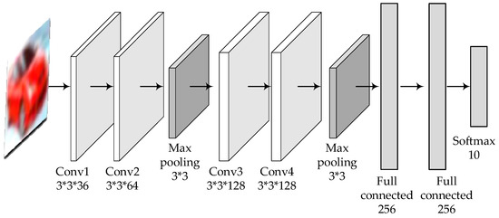
Figure 4.
The structure and parameters of the customized deep learning model for CIFAR-10.
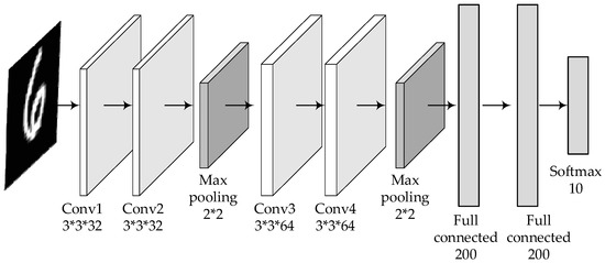
Figure 5.
The structure and parameters of the customized deep learning model for MNIST.
The LeNet, ResNet, and customized deep learning models were trained on the datasets Cifar10 and MNIST, and the image recognition accuracy for the Cifar-10 and MNIST datasets is shown in Table 4. These three models, with their good accuracy, will be used for the subsequent recognition of adversarial examples generated by different algorithms.
Table 4.
Comparison of the accuracy of image recognition classification by different models.
In this paper, when using the Adam optimization algorithm for optimization, the parameters recommended in Reference [23] were used to ensure the optimal performance and effectiveness of experiments, and the validity of the recommended parameter settings was demonstrated in Reference [39]. The initial learning rate is set to 0.001, the exponential decay rate for first-order moment estimation is set to 0.9, and the exponential decay rate for second-order moment estimation is set to 0.999. The constant c is used to prevent the deep learning model from over-fitting the training data. In general, the larger the value of the constant c, the lower the query cost. The experimental results in Reference [14] indicate that the attack time and query frequency are minimized when the value of constant c is set to 10. As a result, in this experiment, the initial value of the constant c is set to 10 after cross-validation.
4.3. Experimental Results and Analysis
This experiment uses the classic algorithms ZOO and One Pixel and the adversarial example generation algorithm proposed in this paper (abbreviated as DE-C&W) to attack three models: LeNet, ResNet, and a custom deep learning model. The performance of the three algorithms in terms of the attack success rate, average attack time, and average number of queries is compared. The results of the experiments on the Cifar-10 dataset and the MNIST dataset are shown in Table 5.
Table 5.
Comparison of experimental results.
Through an analysis of Table 5, it can be seen that the success rates of the proposed algorithm and ZOO algorithm on both the CIFAR-10 and MINIST sets are higher than those of the One Pixel algorithm. This is because the One Pixel algorithm modifies fewer pixels, resulting in relatively weaker attack effects. Although the success rate of the ZOO algorithm on the CIFAR-10 dataset is higher than that of the algorithm proposed in this paper, the ZOO algorithm requires multiple queries to the output of the neural network to obtain reliable results, resulting in a much higher number of queries than the average query times of the algorithm proposed in this paper. Due to the high number of queries in the ZOO algorithm, the attack requires a longer time, which makes it difficult for ZOO to quickly search for the best perturbation when processing high-dimensional images. At the same time, a large number of network query operations also increases the risk of detection. The algorithm proposed in this paper uses the differential evolution algorithm to preprocess images. This algorithm reduces the search dimension of the solution space to a certain extent and can better manage high-dimensional data, while requiring less time and a lower average number of queries than ZOO. In addition, it can be seen that the proposed algorithm can maintain a high success rate on different model architectures and different datasets, which indicates that the algorithm has better transferability. This transferability means that the adversarial examples generated by the algorithm can achieve good attack effects on different deep learning models. Overall, when adversarial attack experiments on three deep learning models on two datasets were conducted, the proposed algorithm not only maintained a high success rate of attacks, but also reduced the average number of queries to the model to varying degrees, reducing the likelihood of attacks being discovered.
In addition, we also calculated the standard deviation of the attack success rate to further validate the effectiveness of the model. The standard deviation of accuracy rates is a statistical measure of how much the accuracy of a model fluctuates over many experiments or different datasets, and it can give us an idea of the stability of the model’s performance. A smaller standard deviation means that the accuracy of the model is relatively stable and its performance fluctuation is small in multiple experiments, which indicates that the model has high stability. For a set of success rates (), the standard deviation of accuracy is calculated as shown in Formula (17).
In this formula, u is the average success rate of attacks on different models, is the standard deviation of accuracy.
In this paper, the standard deviation of each algorithm for different models or datasets is calculated, and the results are compared to analyze the stability of each algorithm, with the results shown in Table 6. The left column of Table 6 compares the standard deviation of attack success rates of the three algorithms on the two datasets, MNIST and Cifar-10, respectively. The right column compares the standard deviation of attack success rates on all datasets. As can be seen in Table 6, the DE-C&W algorithm proposed in this paper performs better in terms of the standard deviation of accuracy overall, indicating its superior stability.
Table 6.
Comparison of standard deviation of accuracy rates.
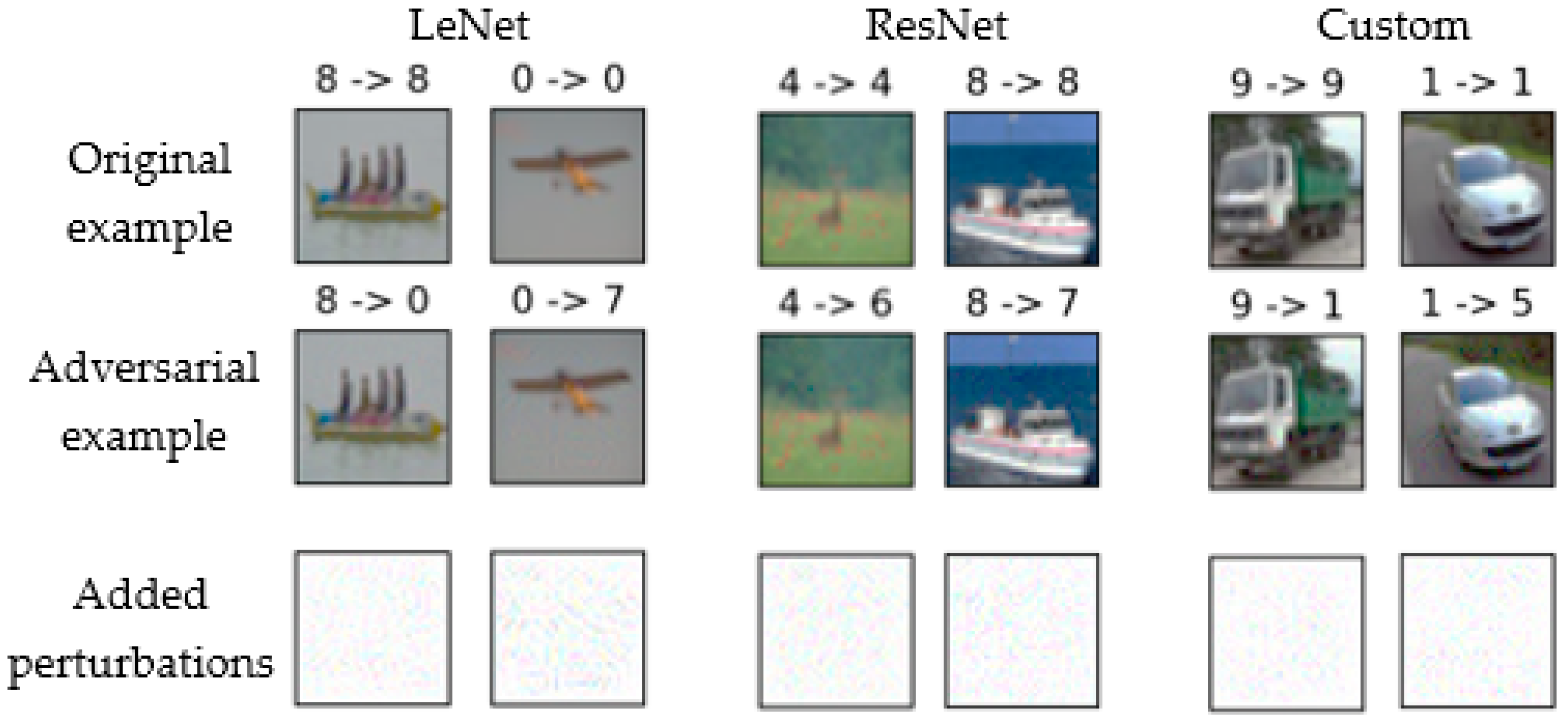
The algorithm proposed in this paper generates optimal perturbations on the MNIST and CIFAR-10 datasets, and conducts adversarial example attacks on LeNet, ResNet, and custom deep learning models. Figure 6 shows some examples of successful attacks on the CIFAR-10 dataset. For example, the correct category for the first image in the first row is 8, corresponding to ship. However, after perturbations were added to the image, it was mistakenly identified as category 0, i.e., airplane. In this figure, the numbers 0 to 9 correspond to airplane, automobile, bird, cat, deer, dog, frog, horse, ship, and truck. Figure 7 shows some examples of successful attacks in the MNIST dataset. For example, the correct category of the first image in the first row is 3, but it was incorrectly identified as 9 after perturbations were added to the image; the correct category of the second image in the first row is 5, but it was also incorrectly identified as 9 after perturbations were added to the image. In this figure, the categories represented by the numbers 0 to 9 correspond to the numbers on the image.

Figure 6.
Examples of successful attacks on the Cifar10 dataset.
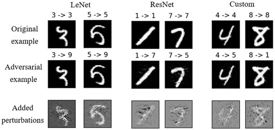
Figure 7.
Examples of successful attacks on the MNIST dataset.
5. Conclusions
In this paper, we investigated a generic algorithm for generating adversarial examples based on DE-C&W. The algorithm preprocesses input images using the differential evolution algorithm to identify sensitive pixels vulnerable to attack, reducing search dimensionality and query times to lower the attack cost. Through the utilization of backpropagation, the adversarial problem is transformed into an optimization problem, optimizing the loss function without requiring access to internal network information for generating universal adversarial perturbations. The Adam optimization algorithm ensures that parameter updates are unaffected by gradient scaling, accelerating convergence. The experimental results demonstrate that our proposed algorithm reduces implementation costs and simplifies the computation process for generating generic adversarial perturbations, thereby enabling efficient, convenient, and cost-effective generic attacks even in scenarios with unknown network structures.
In future work, we aim to further enhance the success rate of adversarial example attacks by incorporating additional optimization algorithms and attack strategies. We also plan to experiment with more complex deep learning models and larger datasets to identify more effective attacks for testing the security of deep learning systems.
Author Contributions
R.Z., Q.W., Y.W. contributed equally to this work. All authors have read and agreed to the published version of the manuscript.
Funding
This work was supported in part by Zhengzhou Collaborative Innovation Project No. 2021ZDPY0106 and Henan Province Science and Technology Research Project No. 252102210183.
Data Availability Statement
The data that support the research findings are provided in the article.
Conflicts of Interest
The authors declare no conflicts of interest.
References
- Jiang, W.; He, Z.; Zhan, J.; Pan, W.; Adhikari, D. Research progress and challenges on application-driven adversarial examples: A survey. ACM Trans. Cyber-Physical Syst. 2021, 5, 39. [Google Scholar]
- Serban, A.; Poll, E.; Visser, J. Adversarial examples on object recognition: A comprehensive survey. ACM Comput. Surv. 2020, 53, 1–38. [Google Scholar]
- Zhang, J.; Li, C. Adversarial examples: Opportunities and challenges. IEEE Trans. Neural Netw. Learn. Syst. 2019, 31, 2578–2593. [Google Scholar] [PubMed]
- Szegedy, C.; Zaremba, W.; Sutskever, I.; Bruna, J.; Erhan, D.; Goodfellow, I.; Fergus, R. Intriguing properties of neural networks. arXiv 2013, arXiv:1312.6199. [Google Scholar]
- Goodfellow, I.J.; Shlens, J.; Szegedy, C. Explaining and harnessing adversarial examples. arXiv 2014, arXiv:1412.6572. [Google Scholar]
- Mao, X.; Chen, Y.; Wang, S.; Su, H.; He, Y.; Xue, H. Composite adversarial attacks. In Proceedings of the AAAI Conference on Artificial Intelligence, Online, 2–9 February 2021; pp. 8884–8892. [Google Scholar]
- Cui, W.; Li, X.; Huang, J.; Wang, W.; Wang, S.; Chen, J. Substitute model generation for black-box adversarial attack based on knowledge distillation. In Proceedings of the 2020 IEEE International Conference on Image Processing, Online, 25–28 October 2020; IEEE: Piscataway, NJ, USA, 2020; pp. 648–652. [Google Scholar]
- Zhang, C.; Benz, P.; Karjauv, A.; Kweon, I.S. Data-free universal adversarial perturbation and black-box attack. In Proceedings of the IEEE/CVF International Conference on Computer Vision, Online, 11–17 October 2021; IEEE: Piscataway, NJ, USA, 2021; pp. 7868–7877. [Google Scholar]
- Kurakin, A.; Goodfellow, I.J.; Bengio, S. Adversarial examples in the physical world. In Artificial Intelligence Safety and Security; Chapman and Hall: London, UK; CRC: Boca Raton, FL, USA, 2018; pp. 99–112. [Google Scholar]
- Moosavi-Dezfooli, S.M.; Fawzi, A.; Frossard, P. Deepfool: A simple and accurate method to fool deep neural networks. In Proceedings of the IEEE Conference on Computer Vision and Pattern Recognition, Las Vegas, NA, USA, 27–30 June 2016; pp. 2574–2582. [Google Scholar]
- Xiao, C.; Li, B.; Zhu, J.Y.; He, W.; Liu, M.; Song, D. Generating adversarial examples with adversarial networks. arXiv 2018, arXiv:1801.02610. [Google Scholar]
- Brendel, W.; Rauber, J.; Bethge, M. Decision-based adversarial attacks: Reliable attacks against black-box machine learning models. arXiv 2017, arXiv:1712.04248. [Google Scholar]
- Chen, P.Y.; Zhang, H.; Sharma, Y.; Yi, J.; Hsieh, C.-J. ZOO: Zeroth Order Optimization Based Black-Box Attacks to Deep Neural Networks Without Training Substitute Models; ACM: New York, NY, USA, 2017; pp. 15–26. [Google Scholar]
- Carlini, N.; Wagner, D. Towards evaluating the robustness of neural networks. In Proceedings of the 2017 IEEE Symposium on Security and Privacy (sp), San Jose, CA, USA, 22–26 May 2017; IEEE: Piscataway, NJ, USA, 2017; pp. 39–57. [Google Scholar]
- Tu, C.C.; Ting, P.; Chen, P.Y.; Liu, S.; Zhang, H.; Yi, J.; Hsieh, C.-J.; Cheng, S.-M. Autozoom: Autoencoder-based zeroth order optimization method for attacking black-box neural networks. In Proceedings of the AAAI Conference on Artificial Intelligence, Honolulu, HA, USA, 27 January–1 February 2019; Volume 33, pp. 742–744. [Google Scholar]
- Su, J.; Vargas, D.V.; Sakurai, K. One pixel attack for fooling deep neural networks. IEEE Trans. Evol. Comput. 2019, 23, 828–841. [Google Scholar]
- Da, Q.; Zhang, G.Y.; Li, S.Z.; Liu, Z.C.; Wang, W.S. Gradient-free adversarial attack algorithm based on differential evolution. Int. J. Bio-Inspired Comput. 2023, 22, 217–226. [Google Scholar] [CrossRef]
- Xie, C.; Zhang, Z.; Zhou, Y.; Bai, S.; Wang, J.; Ren, Z.; Yuille, A. Improving transferability of adversarial examples with input diversity. In Proceedings of the IEEE/CVF Conference on Computer Vision and Pattern Recognition, Long Beach, CA, USA, 15–20 June 2019; pp. 2730–2739. [Google Scholar]
- Huang, L.F.; Zhuang, W.Z.; Liao, Y.X.; Liu, N. Black-box Adversarial Attack Method Based on Evolution Strategy and Attention Mechanism. J. Softw. 2021, 32, 3512–3529. [Google Scholar]
- Hu, W.; Tan, Y. Generating Adversarial Malware Examples for Black-Box Attacks Based on GAN. Data Min. Big Data 2022, 1745, 409–423. [Google Scholar]
- Yang, B.; Zhang, H.; Li, Z.; Zhang, Y.; Xu, K.; Wang, J. Adversarial example generation with AdaBelief optimizer and crop invariance. Appl. Intell. 2023, 53, 2332–2347. [Google Scholar] [CrossRef]
- Liu, Y.; Chen, X.; Liu, C.; Song, D. Delving into transferable adversarial examples and black-box attacks. arXiv 2016, arXiv:1611.02770. [Google Scholar]
- Kingma, D.P.; Ba, J. Adam: A method for stochastic optimization. arXiv 2014, arXiv:1412.6980. [Google Scholar]
- Jais, I.K.M.; Ismail, A.R.; Nisa, S.Q. Adam optimization algorithm for wide and deep neural network. Knowl. Eng. Data Sci. 2019, 2, 41–46. [Google Scholar] [CrossRef]
- Zhang, Z. Improved adam optimizer for deep neural networks. In Proceedings of the 2018 IEEE/ACM 26th international symposium on quality of service (IWQoS), Banff, AL, Canada, 4–6 June 2018; IEEE: Piscataway, NJ, USA, 2018; pp. 1–2. [Google Scholar]
- Storn, R.; Price, K. Differential evolution-a simple and efficient heuristic for global optimization over continuous spaces. J. Glob. Optim. 1997, 11, 341–359. [Google Scholar] [CrossRef]
- Das, S.; Suganthan, P.N. Differential evolution: A survey of the state-of-the-art. IEEE Trans. Evol. Comput. 2010, 15, 4–31. [Google Scholar] [CrossRef]
- Zaharie, D. Critical values for the control parameters of differential evolution algorithms. In Proceedings of the MENDEL 2002, 8th International Conference on Soft Computing, Brno, Czech Republic, 21 May 2002; pp. 62–67. [Google Scholar]
- Gamperle, R. A parameter study for differential evolution. In Advances in Intelligent Systems Fuzzy Systems Evolutionary Computation; Harvard University Press: Cambridge, MA, USA, 2002; pp. 293–298. [Google Scholar]
- Ali, M.M.; Törn, A. Optimization of carbon and silicon cluster geometry for tersoff potential using differential evolution. In Optimization in Computational Chemistry and Molecular Biology: Local and Global Approaches; Springer: Berlin/Heidelberg, Germany, 2000; pp. 287–300. [Google Scholar]
- Gao, X.; Jiang, B.; Zhang, S. On the information-adaptive variants of the ADMM: An iteration complexity perspective. J. Sci. Comput. 2018, 76, 327–363. [Google Scholar] [CrossRef]
- Sun, G.; Yang, B.; Yang, Z.; Xu, G. An adaptive differential evolution with combined strategy for global numerical optimization. Soft Comput. 2020, 24, 6277–6296. [Google Scholar] [CrossRef]
- Fan, Q.; Yan, X. Self-adaptive differential evolution algorithm with zoning evolution of control parameters and adaptive mutation strategies. IEEE Trans. Cybern. 2015, 46, 219–232. [Google Scholar] [CrossRef]
- Elsayed, S.M.; Sarker, R.A.; Essam, D.L. An improved self-adaptive differential evolution algorithm for optimization problems. IEEE Trans. Ind. Inform. 2012, 9, 89–99. [Google Scholar]
- Ghosh, A.; Das, S.; Chowdhury, A.; Giri, R. An improved differential evolution algorithm with fitness-based adaptation of the control parameters. Inf. Sci. 2011, 181, 3749–3765. [Google Scholar]
- Das, S.; Abraham, A.; Chakraborty, U.K.; Konar, A. Differential evolution using a neighborhood-based mutation operator. IEEE Trans. Evol. Comput. 2009, 13, 526–553. [Google Scholar]
- Fan, H.Y.; Lampinen, J. A trigonometric mutation operation to differential evolution. J. Glob. Optim. 2003, 27, 105–129. [Google Scholar]
- Shafiq, M.; Gu, Z. Deep residual learning for image recognition: A survey. Appl. Sci. 2022, 12, 8972. [Google Scholar] [CrossRef]
- Reyad, M.; Sarhan, A.; Arafa, M. A modified Adam algorithm for deep neural network optimization. Neural Comput. Appl. 2023, 35, 17095–17112. [Google Scholar]


Disclaimer/Publisher’s Note: The statements, opinions and data contained in all publications are solely those of the individual author(s) and contributor(s) and not of MDPI and/or the editor(s). MDPI and/or the editor(s) disclaim responsibility for any injury to people or property resulting from any ideas, methods, instructions or products referred to in the content. |
© 2025 by the authors. Licensee MDPI, Basel, Switzerland. This article is an open access article distributed under the terms and conditions of the Creative Commons Attribution (CC BY) license (https://creativecommons.org/licenses/by/4.0/).