Abstract
In this paper, an adaptive iterative Fourier technique (AIFT) algorithm is developed for the synthesis of multiple circular/elliptical beams with low sidelobe levels (SLLs) through phase-only optimization. The key innovation of the AIFT algorithm is the introduction of an elliptical beam model, which facilitates the adaptive determination of main beam regions and offers additional flexibility in controlling pencil beam shapes. Unlike conventional IFT-based algorithms, the AIFT algorithm eliminates the need for prior knowledge of main beam regions and avoids repetitive adjustments of sidelobe correction thresholds. This not only simplifies the configuration process but also prevents the generation of defective radiation patterns. Extensive synthesis experiments with different beam numbers, distributions, and ellipticities demonstrate that the elliptical beam model consistently outperforms its circular counterpart in multibeam scenarios, achieving lower SLL and higher directivity. These advantages are particularly pronounced in asymmetrical beam distributions, highlighting the elliptical beam’s superior potential for reducing SLLs of multi-spot-beam patterns and offering new insights for advancing the performance of point-to-multi-point communication systems.
1. Introduction
Compared with a single-wide-beam antenna, a multibeam array antenna (MBAA) with multiple beams directed toward different directions enables a higher input signal-to-noise ratio (SNR) of the received signal, increased channel capacity, and reduced spectrum congestion [1]. The MBAA is especially suitable for multi-user communication systems, multi-target tracking, imaging radar systems, and integrated sensing and communication systems [2]. The existing approaches developed to realize MBAAs have some limitations, e.g., multiple beams generated at multiple frequencies lead to a waste of spectrum resources [3,4], multiple beams created from different polarizations add significant complexity to element designs [5,6], and even the combination of these two techniques cannot produce more than four beams by one aperture [7,8]. To achieve a large number of simultaneous beams, reflectors or reflectarrays combined with feed arrays were reported in [9,10], but this scheme is too costly and bulky for small satellite applications. Similarly, lens-based multibeam architectures also face issues with bulkiness [11,12]. In recent years, the holographic technique has been utilized to design MBAAs without addressing the suppression of sidelobe levels (SLLs), which is crucial for improving the system’s SNR and spectral efficiency [13,14].
For a regular array composed of elements that have similar structures and low mutual coupling, multiple simultaneous beams of a low SLL can be obtained by simply weighting the amplitudes and phases of array elements, a process known as array synthesis. Phase-only synthesis is of great significance for designing reflectarray antennas, phased arrays, and reconfigurable intelligent surfaces [15,16]. Compared to amplitude-only or amplitude-phase synthesis, phase-only synthesis can obtain higher aperture efficiency and, thus, higher gain [17]. Several works have been done on the phase-only synthesis of MBAAs [18,19,20], but apparently none of them have reached the minimum SLL with relatively uniform sidelobe amplitudes as highlighted in [17].
As a specialized variant of the alternating projection method (APM), the iterative Fourier technique (IFT) enhances computational efficiency by leveraging the Fourier transform pair between the array excitation and array factor [21]. The IFT gained significant recognition in 2007 when Keizer delivered a thorough interpretation and applied it to low-sidelobe synthesis of uniformly spaced planar arrays [22], element failure correction [23], and later, array thinning [24,25,26]. Compared to stochastic or heuristic optimization methods based on evolutionary algorithms [27,28,29,30], IFT offers significant advantages in terms of convergence speed, robustness, and wide applicability to a variety of constraints. Quite a few studies have applied IFT to amplitude-phase synthesis and amplitude-only synthesis [31,32,33,34], whereas few have explored the phase-only synthesis capability of IFT [35], let alone the synthesis of multibeam patterns.
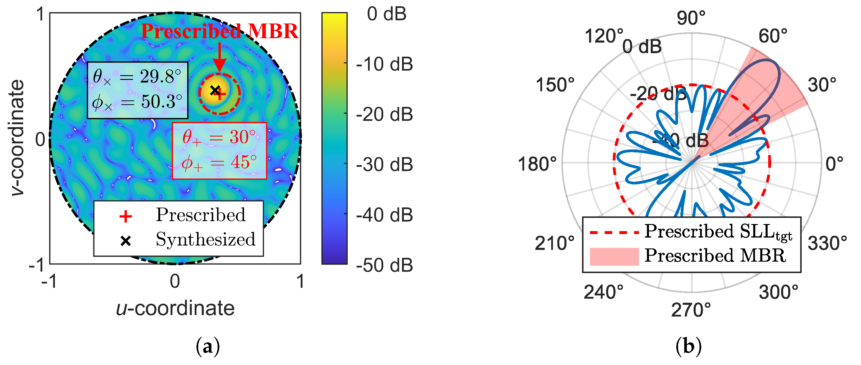
Most existing IFT-based algorithms, including but not limited to those in [35,36,37,38], prescribe a fixed main beam region (MBR) or a predefined mask for the radiation pattern. During synthesis, the sidelobe region (SLR) is depressed while the MBR remains unconstrained, allowing a beam to naturally form in the MBR with reduced SLL due to energy conservation. However, achieving the desired SLL requires multiple attempts with different MBR sizes. If the prescribed MBR is too small, the synthesis will fail to reach the target SLL (). Conversely, if the prescribed MBR is too large, the synthesized pattern may become defective or even invalid, as the lack of constraints within the MBR can result in unintended beam deformations. For example, as shown in Figure 1a, the synthesized beam deviates from the prescribed beam direction, and high sidelobes appear in the prescribed MBR, as shown in Figure 1b.

Figure 1.
A defective radiation pattern synthesized by the IFT due to an over-broad prescribed main beam region (MBR). (a) Pattern in the u-v plane. (b) Pattern at the section.
Moreover, the prescribed MBR over-constrains the solution space and conceivably blocks the possibility of obtaining an even lower SLL pattern that has a slightly different MBR from the prescribed one. Elliptical beams are the universally adopted beams for satellite antennas [39,40,41,42], while circular beams can be considered a special case of elliptical beams with an aspect ratio of one. However, existing low-sidelobe synthesis algorithms primarily focus on reducing the SLLs of strictly circular beams and pay little attention to the relationship between the SLL, beam shape, and beam distribution. As a result, the potential advantages of elliptical beams are often overlooked. This paper aims to fully exploit the degrees of freedom offered by elliptical beams for the low-sidelobe synthesis of multibeam patterns and to investigate the effects of beam distribution and ellipticity on SLL performance.
For multibeam self-adaptation, a challenge is that if there are no additional constraints on the MBRs, only one beam will be formed while the others will gradually collapse to a level close to the sidelobes when the SLR is depressed, regardless of the initial distribution. This indicates that the unconstrained adaptation of the MBR, as demonstrated in [22], is infeasible for multibeam synthesis. To address this issue and ensure the formation of multiple well-defined beams, it is crucial to introduce appropriate constraints on the MBRs. In this paper, we propose an elliptical beam model as the foundation for determining the MBRs, defining pattern constraints, and establishing correction principles, all of which are integrated into the IFT algorithm, resulting in an adaptive IFT (AIFT) algorithm. Unlike previous approaches, the proposed AIFT does not require prior knowledge of beamwidths or achievable SLLs. Instead, it adaptively adjusts the elliptical MBRs based on the results of each iteration and progressively refines the target SLL. Moreover, the AIFT maximally preserves the flexibility of beam shapes in multi-pencil-beam synthesis, opening new possibilities for achieving even lower SLLs.
2. AIFT Algorithm
For a planar array in the x-y plane, the array factor defined in the u-v space (, ) can be expressed as follows:
where represents the complex excitation coefficient of the i-th array element located at , with both coordinates expressed in wavelengths. In phase-only synthesis, the amplitudes of array excitation are predefined, leaving the phases as the only optimization variables.
If the array follows a rectangular lattice, the array factor in (1) can be efficiently computed using the 2D inverse fast Fourier transform (IFFT). The fast Fourier transform (FFT) technique serves as the core computational tool for performing the IFT, enabling rapid transformations between the array excitation and the array factor in pursuit of a low-sidelobe and realizable pattern. Compared to rectangular lattices, triangular lattices offer advantages such as improved cross-polarization isolation and a reduced number of elements required to avoid grating lobes [43]. However, the FFT is inherently designed for rectangular lattices and cannot be directly applied to triangular lattices. Fortunately, since triangular and rectangular lattices are related via affine transformations, and Fourier transforms adhere to specific mathematical rules under such transformations [44,45,46], the FFT can be adapted for triangular-latticed arrays [47]. This capability is integrated into our proposed AIFT algorithm, as detailed in Section 2.1.
The AIFT algorithm retains the fundamental iteration strategy of conventional IFT:
- (i)
- Apply the IFFT to to compute , and then derive the far-field pattern as the product of and the element pattern ;
- (ii)
- Correct according to pattern constraints and then derive the corrected ;
- (iii)
- Apply the FFT to to compute ;
- (iv)
- Correct according to excitation constraints.
The cycle of steps (i)–(iv) continues until both excitation and pattern constraints are satisfied without further correction. At each iteration, the amplitudes of the newly computed are corrected to prescribed array amplitudes at occupied positions and to zero at unoccupied positions, while the phases of remain unchanged for the next iteration.
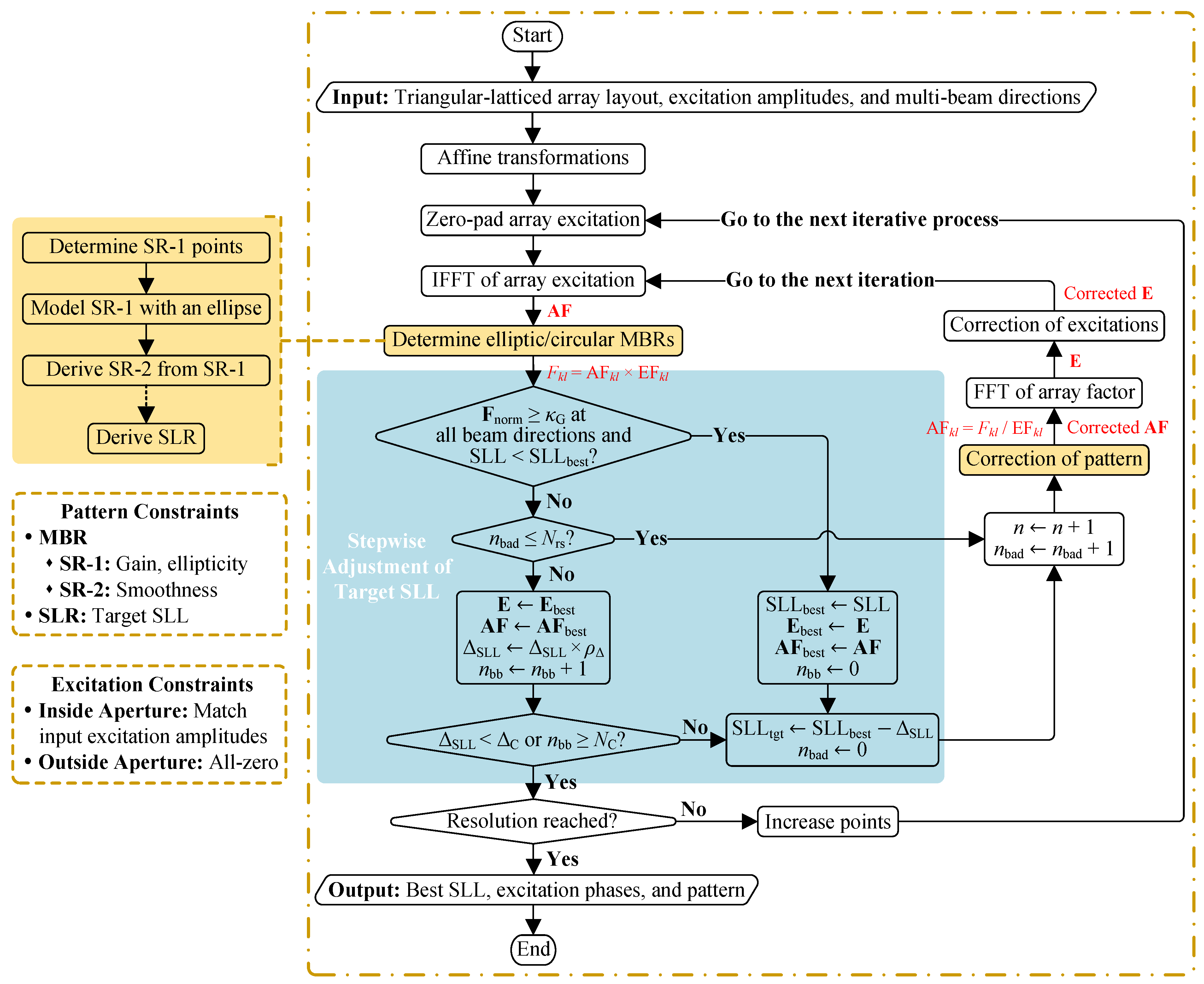
To address the adaptive synthesis of multiple elliptical beams into a pattern with the minimum SLL, two key enhancements are introduced in AIFT, as highlighted in the shaded steps of Figure 2:
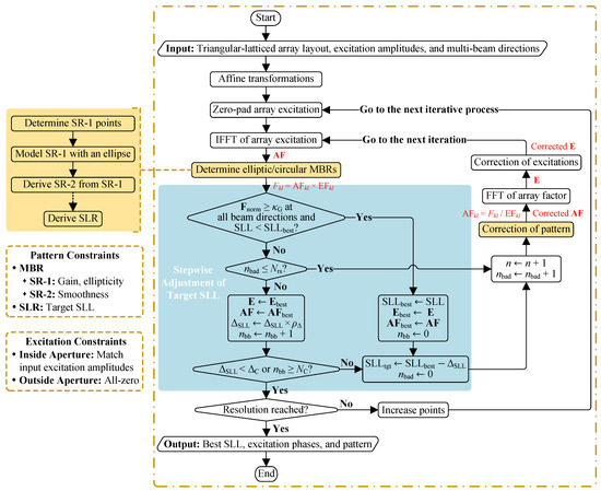
Figure 2.
Flowchart of the proposed AIFT algorithm.
- (i)
- The determination of elliptical MBRs along with the corresponding pattern constraints (shaded in yellow), which will be discussed in Section 2.2 and Section 2.4;
- (ii)
- The rule for updating along with the corresponding convergence conditions (shaded in blue), which will be discussed in Section 2.3.
2.1. Affine Transformations for Triangular Lattices
Consider the triangular lattice illustrated in Figure 3a, where element spacings along the two directions of angle are and , respectively. Affine transformation is imposed on the coordinates of every element to turn this skewed grid into a square grid [48]:
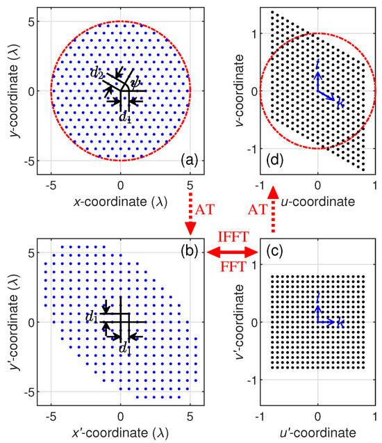
Figure 3.
Schematic diagram of affine transformation applied to the array lattice and its effect on the radiation pattern. (a) Triangular-latticed array, bounded by the red-dotted line. (b) Square lattice obtained after applying an affine transformation to the array. (c) The corresponding lattice of its Fourier pair. (d) Transformed lattice of the radiation pattern, with the visible region bounded by the red-dotted line.
As shown in Figure 3b, after affine transformations, the elements in the new - coordinates will conform to a square grid spaced by , enabling the array excitations to fill in a matrix of rows and columns along and directions, respectively. The corresponding - lattice, i.e., the reciprocal lattice of -, as shown in Figure 3c, is defined as follows:
Now that the array excitation, , expressed in - coordinates, and its array factor, , expressed in - coordinates, fall onto square lattices, we can transform back and forth between and swiftly via FFT:
According to the affine theorem [45], the Fourier pair between triangular lattices x-y and u-v is affine-equivalent to that between the square lattices - and -. Therefore, the array factor of the triangular-latticed array can be derived by simply assigning new coordinates to every matrix element of , i.e., replacing and with u and v, which are calculated as follows (Figure 3d):
To make things clearer, several points must be elucidated:
- To enable radix-2 FFT, M and N need to be raised to integer powers of 2 by zero-padding . For example, a grid should have at least .
- Since grows from , the defined grid does not cover the entire visible region . Acquisition of AF in the undefined u-v area should resort to the periodic nature of FFT.
- The resulting in the skewed u-v lattice, as shown in Figure 3d, can be interpolated into a regular grid if needed.
2.2. Adaptive Determination of Elliptical MBRs
Unlike most array synthesis algorithms, the elliptical MBRs in AIFT are not fixed but adaptively determined in each iteration using an elliptical beam model. The proposed elliptical beam model delineates the elliptical MBRs in the u-v plane, and each MBR is divided into two sub-regions (SRs) for the subsequent establishment of elaborate pattern constraints to form smooth beams.
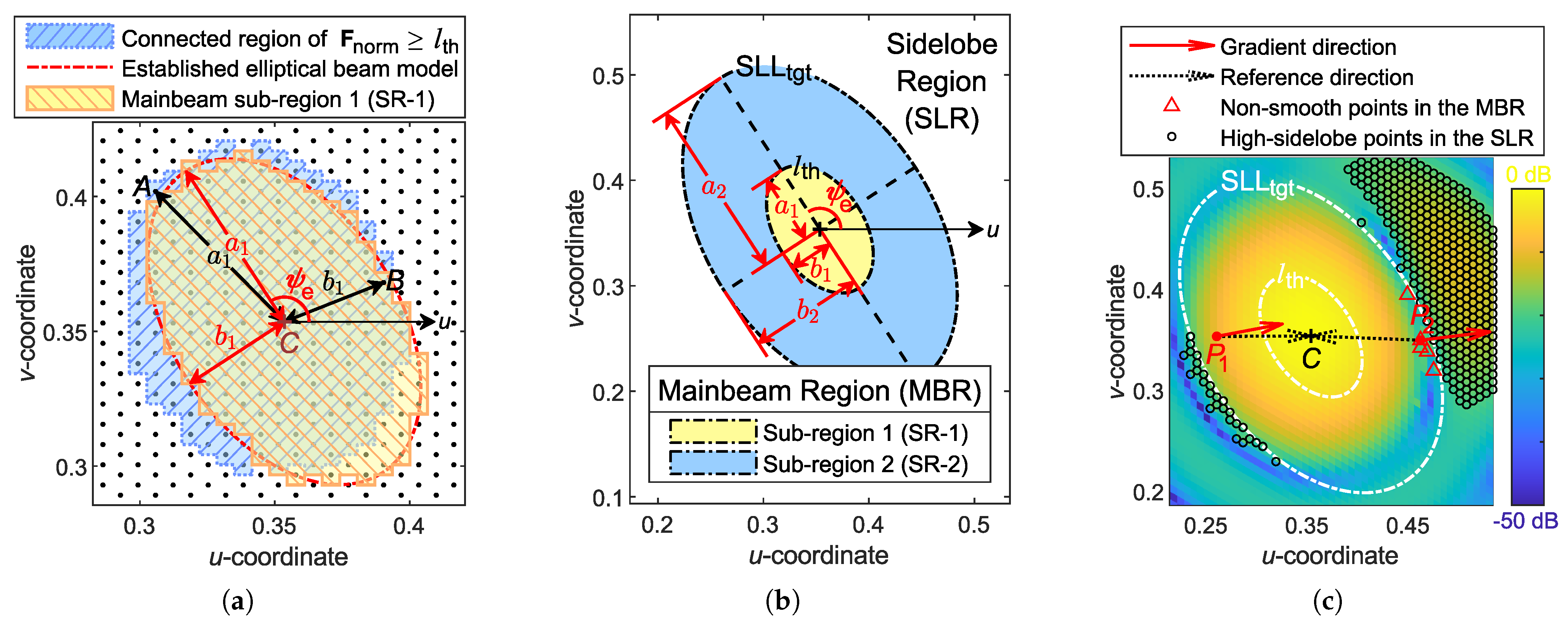
The determination of the MBR involves two major steps, namely, (i) to determine the range of main beam sub-region 1 (SR-1), and (ii) to derive the range of sub-region 2 (SR-2) from SR-1 via the elliptical beam model, as illustrated in Figure 4a and Figure 4b, respectively. The MBR is an elliptical area with the normalized far-field pattern dropping from 1 to , while SR-1 is a smaller area with dropping from 1 to . The remaining annular region inside the MBR and outside of the SR-1 is the SR-2. Due to the unpredictable tailing of the main beam, the model parameters of the elliptical beam are determined based on its inner SR-1. The threshold is dynamically adjusted to maintain a suitable number of points within the SR-1, typically 100–300 points per beam, thus balancing accuracy and computation time.
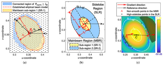
Figure 4.
Schematic illustration of three key steps in the implementation of MBR adaptation. (a) Determination of SR-1. (b) Determination of SR-2 based on SR-1. (c) Points to be corrected in both the MBR and the SLR.
The strategy for determining SR-1 is described below.
- (i)
- Label the points belonging to SR-1:
- Pick out points whose is no less than , i.e., , where the local minima are excluded.
- Find the connected domain without holes from the above-selected set of points centered at the desired beam direction using graph connectivity.
- (ii)
- Use an ellipse to model the SR-1 formed by these points and determine the geometric parameters of the ellipse, as sketched in Figure 4a:
- Among the boundary points of the selected set, find the farthest point A and the closest point B from point C to determine the lengths of the major axis and the minor axis .
- Denotes as the angle between and the u-axis, and as the angle between and the u-axis. The tilt angle of the SR-1 ellipse is determined as follows:where , , and sgn is the signum function.
- (iii)
- The aspect ratio of the elliptical SR-1 is constrained to be no larger than the specified , preventing the beam from becoming overly elongated like a fan beam. If exceeds , the following correction will be performed:
So far, the shape of SR-1 has been determined by , , and . We will show how to calculate the outer boundary of SR-2 (which is also the boundary of the MBR) according to SR-1 in the following.
- (i)
- Assume that the ratio of the major axis to the minor axis is a constant for all elliptic contours of an elliptical beam, i.e., , so that the normalized pattern of an elliptical beam can be modeled as (see Appendix A for derivation procedures):whereand
- (ii)
- The of the already determined SR-1 is used to fit the model (11) and deduce the unknown parameter , which describes the descent rate of the beam’s intensity along the major axis direction of the MBR ellipse.
- (iii)
- (iv)
- Considering that the elliptical model may not completely characterize the exact beam shape, especially for beams with tailing, the final determined MBR is slightly enlarged, as follows:where the variable t (initialized to 1 at the beginning of the synthesis) is adjusted adaptively following a simple strategy: if the proportion of incorrect points in the SR-2 far outweighs that in the SLR, t will be multiplied by a random number slightly smaller than 1, such as 0.95; conversely, if the proportion of incorrect points in the SLR far outweighs that in the SR-2, t will be multiplied by a random number slightly larger than 1, such as 1.05. A smaller t may slow down the search for minimum SLLs, while a larger t may lead to excessive beam broadening. Therefore, t is constrained within the range .
Now that the main beam SRs are determined by repeating the above procedures for all desired beam directions, the SLR is the remaining u-v area after assembling the SRs of all beams. Normally, the determination of MBRs in the AIFT does not need to be done in every iteration as in Figure 2. Instead, it can be done every few iterations—such as five iterations—since the range of main beams may not change significantly within fewer iterations.
Notably, if the elliptical model is simplified to a circular model, (11) will be reduced as follows:
where is the distance from the beam center C to any point in the MBR, describes the decreasing rate of the pattern intensity in all directions originating from C, and is the radius of the circular SR-1. The radius of the circular MBR can be deduced in a way similar to (16) as .
2.3. Stepwise Adjustment of Target SLL
The original IFT algorithm, proposed in 2007 [22], introduced a fundamental pattern correction mechanism where all SLR points with normalized pattern intensity exceeding the target peak sidelobe level were truncated to in each iteration. Subsequent research in 2008 [24] revealed that employing a correction threshold slightly below could achieve superior sidelobe suppression, leading to the concept of the sidelobe threshold (SLT) as formally defined in [33]. While [33] provided preliminary guidelines for SLT selection, the synthesis process still relied on empirical trial-and-error procedures. Additionally, a modified IFT (MIFT) algorithm forcefully lowered the points located at the edge of the MBR to reduce the time cost for linear array thinning [31]. Inspired by the work in [31,33], we find that using a stepwise decreasing can accelerate convergence compared to using a fixed , which also produces lower SLLs and obviates the need for manual adjustment of in search of the minimum SLL. The stepwise adjustment procedures are systematically illustrated in the flowchart highlighted in blue in Figure 2, a detailed explanation of which shall be provided below.
During the iterative process, the best results so far are saved in memory, including , corresponding array excitation , and array factor . A maximum of iterations is allowed for each value, and the number of non-contributing iterations is counted by the variable . Each time the acceptable gain difference is met for all the beams, except for the first iteration of each iterative process, AIFT checks whether to update . If the current SLL is not lower than and the maximum iteration number of a single is not reached, will remain the same in the next iteration. If the current , i.e., better results are obtained, the best results in memory will be updated with the current results, and will be lowered to . If reaches , the best results in memory will be reloaded into the iterative process. In this case, will be multiplied by a reduction factor , and will be updated to . The variable counts consecutive rounds of reaching , with a maximum of . If consecutive updates to do not produce a better result, or , the iterative process terminates, where is the specified convergence criterion.
Due to the nature of FFT, the number of points in both the x-y plane and the corresponding u-v plane is the same, like . For accurate pattern corrections, K should be large enough to produce a far-field pattern with sufficient resolution. But starting with a large K is not ideal, as it leads to longer computation times in finding a reasonable distribution and increases the risk of becoming trapped in local minima. We prefer to start with a smaller K, which will be increased once the iterative process converges at the current resolution. The larger-K iterative process then takes the from the smaller-K process as its initial array excitation, and the process continues until the convergence condition is met with the pattern resolution specified by .
The overall synthesis consists of several rounds of iterative processes, with K progressively increased round by round. At the beginning of each iterative process, the counter for a single and the iteration number n will be set/reset to 1. In practice, we found that initialized to 2– would be a good choice for the most part. The reduction factor , which determines the decreasing speed of , is set larger (e.g., 0.7) for the initial smaller-K iterative process to allow for more iterations in search of better results. For subsequent larger-K iterative processes, is set smaller (e.g., 0.5) to reduce iterations and save time. The variables , , and are initialized in the first iteration of each iterative process as , , and , respectively. They will approach better results through the iterative process and will be updated with higher resolution as K increases. The suggested values for some constant parameters are as follows: , , , and . Decreasing , , or , or increasing will reduce the number of iterations required for convergence; however, this may also decrease the likelihood of achieving lower SLLs.
2.4. Radiation Pattern Correction
Until the convergence condition is met, radiation pattern correction is conducted in each iteration for all the MBRs and the SLR to achieve smooth pencil beams with a lower SLL. For multibeam synthesis, the beams may become non-smooth during synthesis, while the non-smooth points on the beams contribute to the SLL. Therefore, pattern constraints should be applied to each MBR, as listed below, to achieve two goals: (i) to ensure that the beams will not collapse during the adaptive iterations, and (ii) to maintain the smoothness of the beams during the iterations.
- (i)
- .
- (ii)
- ,
As explained before, multiple beams cannot be formed spontaneously via adaptive iterations when suppressing the SLR. To solve the beam collapse problem, i.e., multiple beams degenerate into a single beam during iterations, the maximum gain difference between beams is restricted to a given , which guarantees that multiple beams have a similar gain, and therefore the problem of beam collapse can be avoided. Specifically, for multibeam synthesis, the normalized pattern intensity in any given beam direction should not be lower than ; otherwise, all points within SR-1 of this beam will be corrected to 1 in this iteration.
The parameter is introduced as a constraint to ensure beam smoothness. Since the final determined MBR is slightly larger than the actual one (to accommodate unpredictable beam tailing), sidelobes may appear in SR-2. Therefore, only points within SR-2 with are evaluated for smoothness, ensuring that the beam remains smooth and that any potential sidelobes in SR-2 do not exceed . For an idealized pencil beam, decreases in all directions from the beam center to the boundary of the MBR. That is, the gradient direction at every point on the beam (except the beam center) should point toward the beam center with a declination smaller than . A small , e.g., , can keep the beams smooth but limits the beam shape, resulting in an effect equivalent to using the circular beam model (20) and reducing the possibility of obtaining even lower SLLs. Therefore, is recommended to be between and to ensure smooth beams while preserving the maximum freedom for beam shapes. Take the pattern of Figure 4c as an example: and are two points in SR-2. The reference direction goes from (or ) to the beam center C. While the gradient direction of basically matches its reference direction, the gradient direction of deviates from its reference direction by more than , which means is not smooth at and needs to be corrected. For each non-smooth point, its correction value is determined by the elliptical beam model defined by (11). We can rewrite it here as follows:
where and are figured out in (12)–(15).
The constraint for the SLR is straightforward: ,
As shown in Figure 4c, points in the SLR with are marked as “high-sidelobe points in the SLR” and are required to be corrected to , a random value between and . Although minor variations in have negligible impact on the final SLL, this controlled randomization enhances solution diversity and facilitates escape from local optima.
It is worth emphasizing that the sidelobe level is the maximum value of for all the points in the SLR and the non-smooth points in the MBR. The above three pattern constraints can guarantee multiple smooth pencil beams while maximally preserving the freedom of adaptive MBRs. With all pattern constraints applied, the beam centers of the synthesized pattern will lie exactly in specified directions, and the deviation will not exceed the grid size of the u-v plane in which it is being synthesized.
3. Results and Analysis
In this section, several single-beam and multibeam synthesis examples using the elliptical beam model with different aspect ratios will be presented and the results will be analyzed. For comparison, all examples are based on the following premises.
- Phase-only synthesis for arrays with equal excitation amplitudes, initialized with uniform amplitude and phase distributions.
- Omnidirectional array elements are arranged in an equilateral triangular lattice with element spacing , as shown in Figure 3a.
- A single iterative process is restricted to no more than iterations.
- The aspect ratios of the beams are limited to a maximum of . For multibeam synthesis, the maximum gain difference between beams is constrained to .
- Beam directions are listed below, which will be combined to form different beam sets:
- –
- Beam ⓪: ;
- –
- Beam ①: , ;
- –
- Beam ②: , ;
- –
- Beam ③: , ;
- –
- Beam ④: , .
3.1. Single-Beam Synthesis
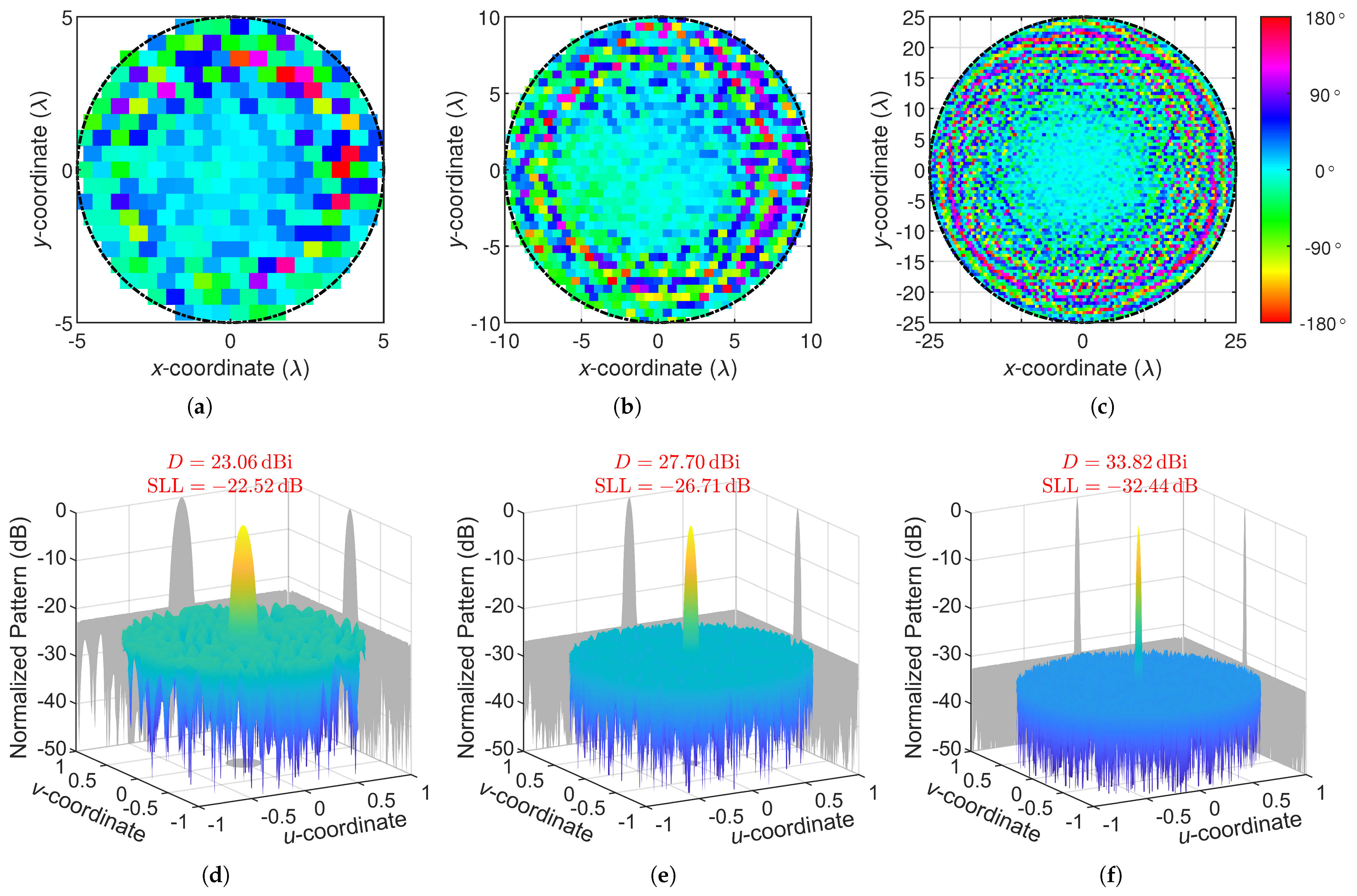
To demonstrate that the beam-adaptation characteristic does not hinder the search ability of the algorithm, single-beam patterns with different aperture diameters were synthesized using both our proposed AIFT and the MIFT [33], while the MIFT can be considered as a version of AIFT without self-adaptation functionality. The single-pencil-beam patterns synthesized by AIFT and their corresponding phase distributions are presented in Figure 5. The -diameter circular array contains 253 elements, the array has 1015 elements, and the array has 6307 elements. In all three cases, roughly uniform energy distributions are achieved in the SLRs, indicating that the minimum SLLs obtained by AIFT are either local optima or at least very close to local optima [17].

Figure 5.
Phase distributions (a–c) correspond to the synthesized single-beam patterns (d–f) of , , and aperture diameters, respectively.
Detailed metrics are listed in Table 1, where the beamwidths are calculated in two principal planes [49] with respect to each beam, and the aspect ratios of the synthesized beams are also listed for comparison. The aspect ratio of the elliptical main beam footprint for AIFT synthesis is constrained to , which is the maximum allowable aspect ratio for self-adaptation. However, despite the freedom given to the aspect ratio, all beams synthesized by AIFT have aspect ratios smaller than 1.1, i.e., they are very close to circular beams, which means that the advantage of the elliptical beam model is not shown in single-beam synthesis. That is to say, a circular beam is better than an elliptical beam for achieving low SLL in single-beam synthesis. For all three aperture sizes, the proposed AIFT realizes basically the same SLLs and beamwidths as the MIFT, showing that the AIFT has a comparable search ability to MIFT in single-beam synthesis and the beam-adaptation characteristics do not affect the search ability of AIFT.

Table 1.
Synthesis results for beam #0 obtained by MIFT and AIFT.
3.2. Multibeam Synthesis
To verify the superiority of adaptive elliptical beams over circular beams in multibeam synthesis, different beam sets are synthesized on a -diameter array. The maximum gain difference between beams is set to . For all synthesized beams, the aspect ratio of each beam can be any value between 1 and . Figure 6 shows three typical multibeam patterns and the corresponding phase distributions synthesized by AIFT with . Due to the adaptivity provided by AIFT, the synthesized beams within a pattern can differ in aspect ratio, tilt angle, and beamwidth—precisely the tunable parameters essential for achieving lower SLLs. These critical degrees of freedom, however, remain largely untapped in previous IFT implementations constrained by prescribed MBRs.
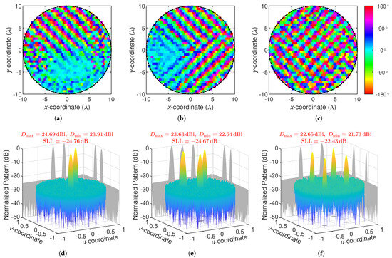
Figure 6.
Phase distributions (a–c) corresponding to the synthesized multibeam pattern of beams (d) ⓪①, (e) ⓪①②, and (f) ①②③④, respectively.
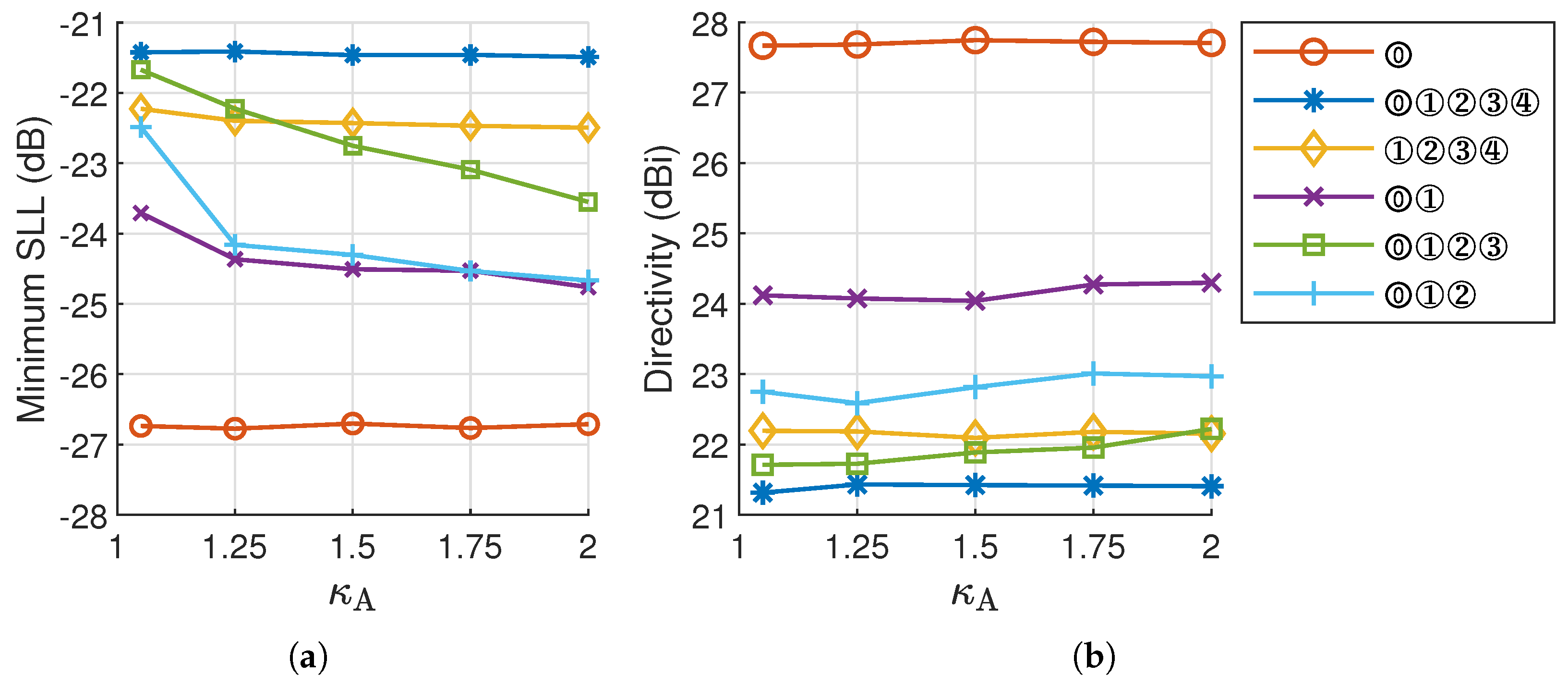
In the following, experiments are conducted separately on five beam sets with the beam number ranging from 2 to 5, viz., beam sets ⓪①, ⓪①②, ⓪①②③, ①②③④, and ⓪①②③④. For each beam set, five values ranging from 1.05 (i.e., nearly circular beam) to 2 are tested, and 50 trials are carried out for each value. Figure 7 presents the minimum SLL obtained from 50 trials, along with the corresponding mean directivity of the beam set.
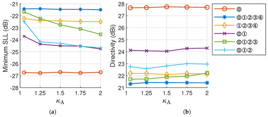
Figure 7.
Synthesis results of a -diameter array for different beam sets and values: (a) minimum SLL and (b) corresponding directivity.
The MBRs gain greater flexibility in aspect ratios by increasing . As shown in Figure 7, for the beam sets ⓪①② and ⓪①②③, an SLL reduction of approximately 2 dB is achieved as increases from 1.05 to 2, accompanied by a slight improvement in directivity. The experiment results confirm the potential of reducing SLL by using elliptical MBRs instead of circular ones. For beam set ⓪①, an SLL reduction of approximately 1 dB is achieved. However, for beam sets ①②③④ and ⓪①②③④, little improvement is observed as increases. All the experiment results indicate that while elliptical beams are advantageous in lowering the SLL of multibeam patterns, their effectiveness in reducing the SLL varies with different beam configurations.
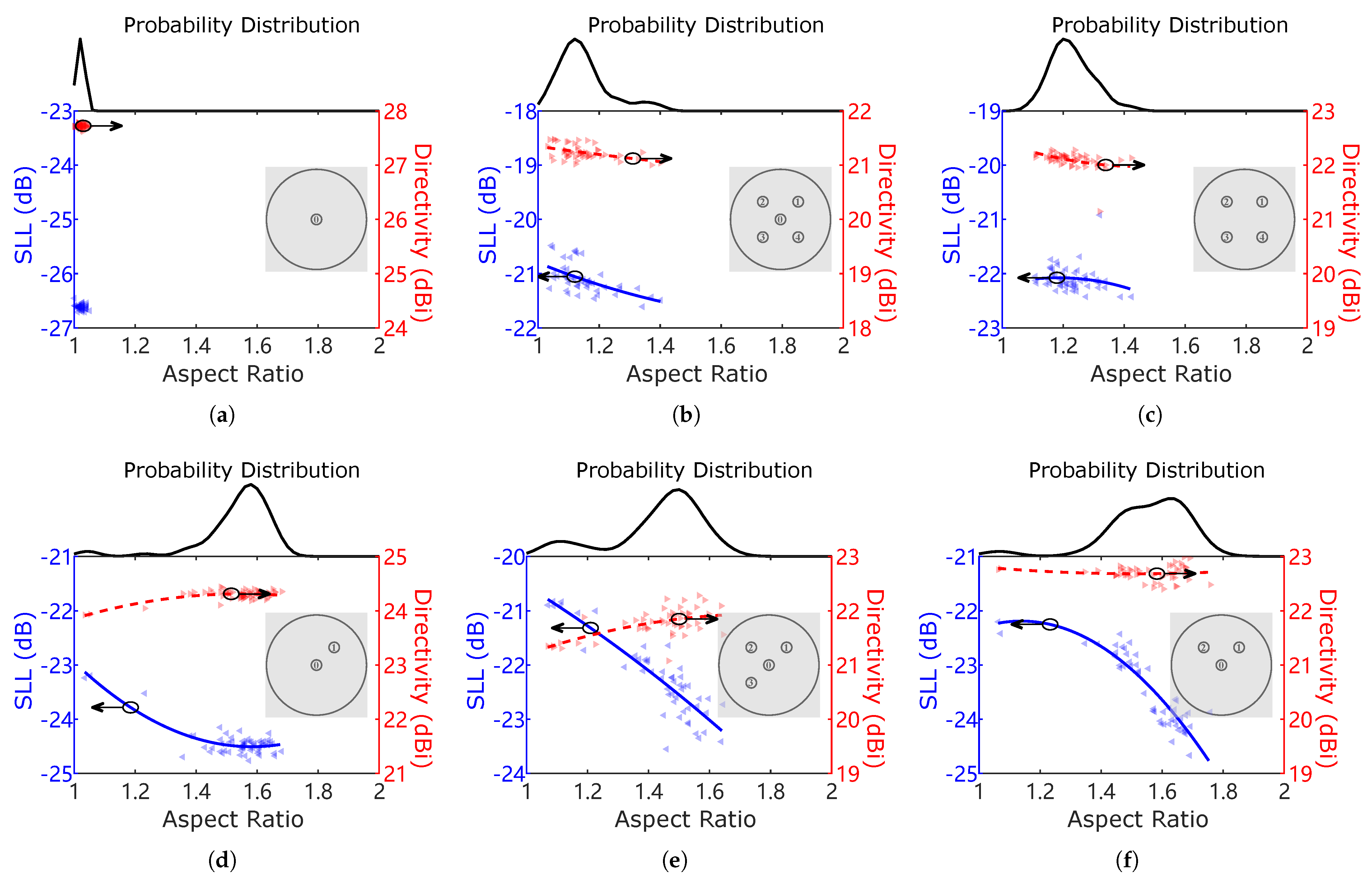
Figure 8 presents the results of 50 runs for each beam set synthesized by AIFT under the aspect ratio constraint , with an inset showing the corresponding beam distribution in the u-v plane. For each run, scatter plots illustrate the relationship between the mean aspect ratio of the synthesized beam set, SLL, and mean directivity, with fitting curves included for enhanced clarity. Additionally, the upper portion of each diagram displays the probability density distribution of the aspect ratios derived from the 50 runs.
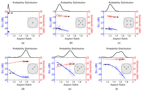
Figure 8.
SLL, mean directivity, and mean aspect ratio of patterns synthesized on a -diameter array for beam sets (a) ⓪, (b) ⓪①②③④, (c) ①②③④, (d) ⓪①, (e) ⓪①②③, and (f) ⓪①②. For each beam set, results for 50 runs of the AIFT algorithm with are shown as scatter points along with fitting curves. The top of each diagram plots the probability density distribution of the aspect ratios across all 50 runs.
In the single-beam synthesis cases, a near-circular beam is consistently formed in every trial despite the use of adaptive elliptical shaping, as represented by the patterns in Figure 5. Consequently, all aspect ratios from the 50 runs are close to 1, leading to a sharp peak at 1 in the probability plot of Figure 8a. In the multibeam synthesis cases illustrated in Figure 8b–f, there is a negative correlation between SLLs and the mean aspect ratios of multiple beams. By comparing the probability density distributions with the beam distributions, it is evident that more asymmetrical beam distributions, as in Figure 8d–f, tend to produce higher aspect ratios (above 1.5) in the adaptive synthesis. Such patterns, as exemplified in Figure 6d,e, exhibit highly elliptical beams. The increase in aspect ratio is accompanied by a significant SLL reduction, indicating that the degrees of freedom provided by adaptive elliptical beams in AIFT have been effectively utilized. In contrast, more symmetrical beam sets, as illustrated in Figure 8b,c, exhibit smaller SLL reductions and aspect ratios concentrated below 1.2. This suggests that the degree of freedom in beam ellipticity is underutilized and the benefit of elliptical beams is less pronounced in synthesizing symmetric beam sets. As exemplified in Figure 6f, such patterns are less elliptical.
In the following analysis, we will examine the detailed results. Comparing the four-beam sets ⓪①②③ and ①②③④, it is evident that the more asymmetric set ⓪①②③ can achieve a further reduction in SLL by using elliptical MBRs, while the more symmetric set ①②③④ shows less distinctive results as varies. When all MBRs are restricted to be close to circular (i.e., ), the more symmetric beam set ①②③④ achieves an SLL that is 1 dB lower than set ⓪①②③. However, when greater shape flexibility is allowed for MBRs (i.e., ), the more asymmetric beam set ⓪①②③ achieves an SLL that is 2 dB lower than set ①②③④. Overall, for low-sidelobe multibeam synthesis with the same number of beams, the performance hierarchy is as follows: asymmetric beam distributions with elliptical beams outperform symmetric beam distributions with elliptical beams, which in turn surpass symmetric beam distributions with circular beams, followed by asymmetric beam distributions with circular beams.
It is well-established that patterns with minimum SLLs typically exhibit a uniform energy distribution across the SLR [17]. Different beam sets primarily differ in their energy distributions, and the shape of individual beams further influences the energy distributions. To assess the uniformity of energy distribution across beam sets, the number of symmetry axes serves as an effective metric—a beam set with more symmetry axes corresponds to a more uniform energy distribution in the azimuthal direction. Notably, the absolute position of a beam set in the u-v plane does not affect energy uniformity; rather, symmetry is determined solely by the relative positions of the beams, as the u-v plane can be periodically extended infinitely in any direction.
A single-beam configuration possesses an infinite number of symmetry axes, achieving the highest possible symmetry—surpassing that of any multibeam set. Likewise, a circular beam exhibits the highest symmetry among all beam shapes, best preserving the uniformity of a single-beam pattern and, thus, yielding the lowest SLLs. In contrast, multibeam configurations, characterized by dispersed MBRs across the u-v plane, inherently disrupt SLR symmetry and create uneven energy distributions. In such cases, elliptical beams provide additional degrees of freedom, including beam ellipticity and tilt angle, which are lacking in circular beams. These extra degrees of freedom enable more adaptable beam arrangements, helping to improve the uniformity of energy distribution. Consequently, beam sets with fewer symmetry axes—indicating greater inherent asymmetry—achieve more significant SLL reductions when elliptical beams are used instead of circular ones, as demonstrated in Figure 7, Figure 8 and Figure 9.
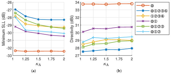
Figure 9.
Synthesis results of a -diameter array for different beam sets and values: (a) minimum SLL and (b) corresponding directivity.
The symmetry axes associated with the synthesized beam sets mentioned above can be summarized as follows:
- A single beam has countless symmetry axes.
- A beam set of two beams has two symmetry axes.
- A beam set of three beams may have 1 to 3 symmetry axes based on its beam distribution, e.g., the beam set ⓪①② in Figure 8f has 1 symmetry axis.
- A beam set of five beams may have 1 to 5 symmetry axes, e.g., the beam set ⓪①②③④ in Figure 8b has 4 symmetry axes.
Therefore, the symmetry of the above beam sets can be ranked as follows: ⓪ > ⓪①②③④ ≈ ①②③④ > ⓪① > ⓪①②③ ≈ ⓪①②. We can conclude that beam sets with fewer symmetry axes benefit more from elliptical MBRs, achieving greater SLL reduction by exploiting beam ellipticity, as clearly demonstrated in Figure 7 and Figure 9. It should be noted that while the number of symmetry axes serves as a general measure of symmetry, beam sets with the same number of symmetry axes (e.g., ⓪①② and ⓪①②③) may still exhibit slight differences in symmetry due to their different distributions.
We extend the experiments to a -diameter array, with the results summarized in Figure 9. The synthesized patterns for the larger array exhibit trends similar to those observed in the -diameter case. Similar trends are also observed in the -diameter array synthesis; however, these results are omitted for brevity.
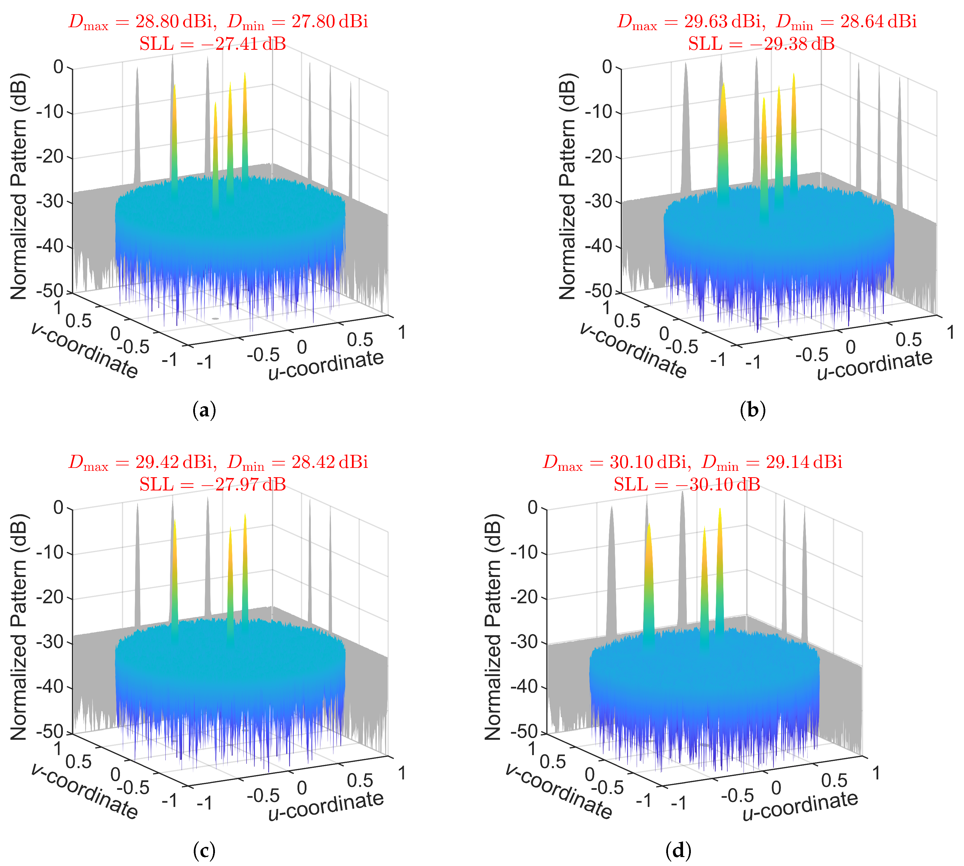
The -diameter array achieves more pronounced SLL reductions and enhanced directivity across all tested beam sets as increases from 1.05 to 2. Specifically, for beam sets ⓪①②③ and ⓪①②, as shown in Figure 10, the SLL is further reduced by 1.97 dB and 2.13 dB, respectively, while simultaneously achieving mean directivity improvements of 0.8 dB and 0.7 dB. These enhancements indicate that more energy is effectively concentrated in the desired beam directions.

Figure 10.
Minimum SLL patterns for beam set ⓪①②③ under the constraint of (a) and (b) , and for beam set ⓪①② under the constraint of (c) and (d) , synthesized on a -diameter array.
We now examine the convergence performance of the proposed algorithm through two representative cases: single-beam synthesis for beam ⓪ and multibeam synthesis for beam set ⓪①②. Figure 11 compares the convergence behavior of AIFT using two strategies: stepwise-adjusted (stepwise target) and fixed (fixed target). During the iterative process, denotes the best found up to that iteration, while the target is either stepwise reduced (stepwise target) or fixed at a minimum value throughout (i.e., fixed target). Achieving an SLL close to the lowest value is relatively easy, but obtaining the final 0.5 dB reduction requires thousands of iterations. As shown in Figure 11a, for single-beam synthesis, the fixed-target strategy leads to a faster decrease in during the early iterations, making it suitable when an acceptable SLL is sufficient and faster convergence is desired. In contrast, Figure 11b shows that for multibeam synthesis, the stepwise-target strategy not only accelerates the early-stage reduction of but also ultimately achieves a lower final than the fixed-target strategy, demonstrating its superior search capability. Overall, for single-beam synthesis, the number of iterations can be minimized if is empirically set close to the minimum SLL from the outset. However, in multibeam synthesis, a fixed fails to reach the lowest SLL, whereas a stepwise-adjusted offers better performance in terms of both iteration efficiency and final SLL reduction.
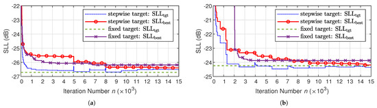
Figure 11.
Comparison of the convergence speed of AIFT with and without a stepwise adjustment in through iterations of (a) single-beam synthesis and (b) multibeam synthesis on a -diameter array.
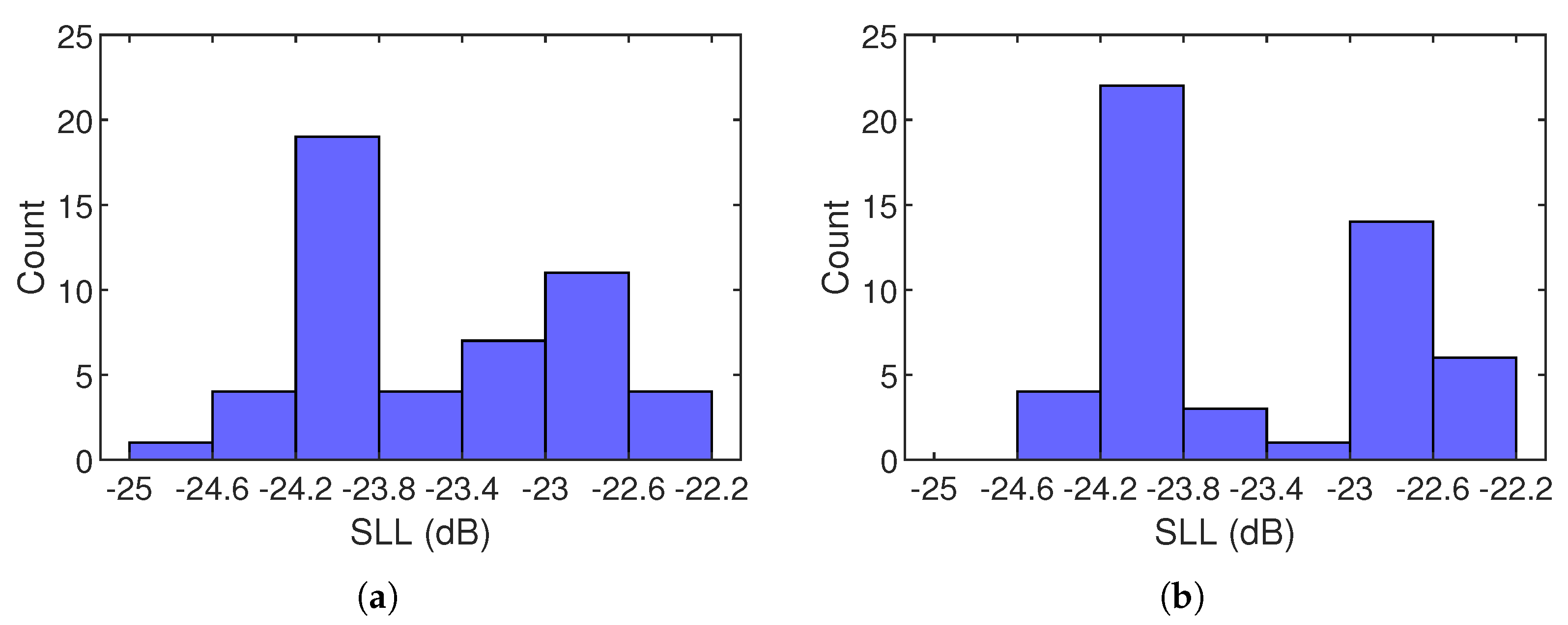
To evaluate the algorithm’s robustness against local optima, we conducted comparative experiments on beam set ⓪①②, which has the largest variation in synthesized SLLs among all tested beam sets, as shown in Figure 8f. A total of 50 runs are performed using a uniform random initial phase distribution, and the results are compared to those obtained from the uniform initial phase distribution presented earlier in Figure 8f, as illustrated by the comparative histograms in Figure 12. In both cases, the most frequently observed SLL is approximately , very close to the global optimum of . This suggests that the algorithm is largely insensitive to the choice of initial values and can effectively escape from narrow and shallow local optima. However, the observed fluctuation of approximately between the best and worst SLLs indicates that the algorithm occasionally becomes trapped in certain local optima. Nonetheless, this variation is acceptable given the algorithm’s inherent adaptivity and controlled randomness.

Figure 12.
Histograms of synthesized SLLs for beam set ⓪①② on a -diameter array over 50 runs with (a) a uniform initial phase distribution and (b) a random initial phase distribution.
Notably, a secondary peak emerges around in both cases, corresponding to smaller aspect ratios, as illustrated in Figure 8f. This suggests that the algorithm sometimes stagnates at lower ellipticities, forming broad and deep local optima. To address this, a simple yet effective solution is to impose a lower bound on the beam aspect ratio, ensuring AIFT consistently generates highly elliptical beams with minimized SLLs. Specifically, for highly asymmetrical configurations with fewer than three symmetry axes, we recommend constraining the aspect ratio to a higher range (e.g., ), which enhances robustness and prevents convergence to local optima associated with near-circular beams. For more symmetric configurations with more than three symmetry axes, limiting the aspect ratios to a lower range (e.g., ) can promote faster convergence while maintaining optimal performance.
4. Conclusions
We propose using the elliptical beam model to characterize the shape of pencil beams, capitalizing on the superior flexibility of elliptical beams over circular ones to reduce SLLs. This model forms the foundation for sophisticated pattern constraints and correction mechanisms that ensure beam smoothness and stability during adaptive iterations, facilitating MBR adaptation for synthesizing multiple circular or elliptical beams. By incorporating a stepwise-adjusted target SLL, the proposed AIFT algorithm achieves a fully adaptive synthesis of multiple pencil beams with minimized SLLs. Given the desired beam directions, the AIFT algorithm can automatically determine the pattern with the lowest SLL without the need to prescribe MBRs or attempt different sidelobe correction thresholds.
For single-beam synthesis, AIFT consistently generates circular beams, even when employing an adaptive elliptical MBR, indicating that a circular beam shape is optimal for minimizing SLLs of single-beam patterns. In contrast, for multibeam synthesis, elliptical beams significantly outperform circular ones, especially in asymmetrical beam arrangements. As the aspect ratios of the MBR ellipses increase, SLLs are further reduced, directivity improves slightly, and more asymmetrical beam distributions benefit increasingly from the ellipticity. This improvement stems from the ability of adaptive elliptical beams to adjust their tilt angles and aspect ratios to better counteract asymmetry. Based on these insights, we propose constraining the aspect ratios of adaptive elliptical beams to higher values for low-sidelobe synthesis of highly asymmetric multibeam configurations, while adopting lower aspect ratios for more symmetric configurations. This strategy ensures faster convergence while reducing the risk of local optima.
Future research should explore integrating heuristic algorithms to further unlock the potential of elliptical beams for SLL reduction in multibeam patterns [34,50], while machine learning-based pre-trained models offer a promising path toward real-time synthesis and improved computational efficiency [51,52]. Additionally, the demonstrated effectiveness of elliptical beams in low-sidelobe phase-only synthesis suggests their application in amplitude-phase synthesis warrants further investigation. To enhance real-world performance, practical factors such as mutual coupling, edge effects, array position variations, and excitation errors should also be carefully addressed, either proactively or as part of the synthesis process [53,54].
Author Contributions
Conceptualization, Y.D. and X.Z.; data curation, Y.D.; formal analysis, Y.D., Y.Z. and X.Z.; funding acquisition, Y.Z. and X.Z.; investigation, Y.D. and X.Z.; methodology, Y.D., Y.Z. and X.Z.; project administration, Y.Z. and X.Z.; resources, Y.D., Y.Z. and X.Z.; software, Y.D.; supervision, Y.Z. and X.Z.; validation, Y.D.; visualization, Y.D.; writing—original draft, Y.D.; writing—review and editing, Y.D., Y.Z. and X.Z. All authors have read and agreed to the published version of the manuscript.
Funding
This research was funded in part by the National Natural Science Foundation of China (grant no. 61901451) and the Youth Innovation Promotion Association of the Chinese Academy of Sciences (grant No. 2022148).
Institutional Review Board Statement
Not applicable.
Informed Consent Statement
Not applicable.
Data Availability Statement
The original contributions presented in this study are included in the article. Further inquiries can be directed to the first author.
Conflicts of Interest
The authors declare no conflicts of interest.
Abbreviations
The following abbreviations are used in this manuscript:
| SLL | sidelobe level |
| IFT | iterative Fourier technique |
| AIFT | adaptive iterative Fourier technique |
| FFT | fast Fourier transform |
| IFFT | inverse fast Fourier transform |
| MBAA | multibeam antenna array |
| MBR | main beam region |
| SR-1 | sub-region 1 |
| SR-2 | sub-region 2 |
| SLR | sidelobe region |
Appendix A. Derivation of the Elliptical Beam Model
The model is commonly used for shape descriptions of pencil beams [55]. For a circular beam, a model is sufficient to describe its shape, as the beam is rotationally symmetric and has the same pattern profile for all cuts. However, for an elliptical beam, due to the differing rate of the beam intensity falling from the center to the edge in different directions, even if two models are used to describe the pattern profiles of the major axis direction and minor axis direction, the pattern profiles in directions other than these two are still undefined. To this end, we propose an elliptical beam model to determine the beam intensity at any point in the u-v plane. By converting the of each point into an equivalent major axis or an equivalent minor axis , all points in the u-v plane are classified into elliptic contours with varying intensities.
As sketched in Figure 4b, SR-1 is modeled as an ellipse with major axis , minor axis , and tilt angle in the u-v plane. Let us define a new coordinate system - with as the origin, and and along the major and minor axis directions of the ellipse, respectively. The new coordinates are thus obtained by translating and rotating :
Suppose that the elliptical beam fades with along the major axis direction and along the minor axis direction, where and can be deduced from the already determined SR-1:
The contours of the elliptical beam are ellipses that gradually spread outward from and never join. Each point in the - plane should lie on an elliptic contour, distinguished by its major axis or minor axis , which can be obtained by solving the following equation set:
Considering that (A5) has no analytical solution, of an elliptical beam is regarded as a constant value for simplicity, thus (A5) can be simplified as
The model representing the normalized pattern of the elliptical beam within the MBR is thereby established as
or
Either (A9) or (A10) can be used to delineate an elliptical beam, as exemplified in Figure A1, where is determined at the SR-1 boundary. However, it is important to note that, strictly speaking, the aspect ratio of the elliptic contour varies slightly with changes in . Consequently, the patterns defined by (A9) and (A10) may exhibit slight differences due to the approximation of as a constant.
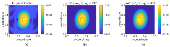
Figure A1.
Modeling an elliptical beam using the proposed elliptical beam model, with the red-dotted line indicating the boundary of SR-1 for deriving model parameters. (a) Original pattern with the elliptical beam. (b) Elliptical beam model derived from (A9). (c) Elliptical beam model derived from (A10).

References
- International Telecommunication Union. The Last-Mile Internet Connectivity Solutions Guide: Sustainable Connectivity Options for Unconnected Sites; ITU: Geneva, Switzerland, 2020. [Google Scholar]
- Zhuo, Y.; Mao, T.; Li, H.; Sun, C.; Wang, Z.; Han, Z.; Chen, S. Multi-Beam Integrated Sensing and Communication: State-of-the-Art, Challenges and Opportunities. arXiv 2024. [Google Scholar] [CrossRef]
- Smith, T.; Gothelf, U.; Kim, O.S.; Breinbjerg, O. An FSS-backed 20/30 GHz Circularly Polarized Reflectarray for a Shared Aperture L- and Ka-band Satellite Communication Antenna. IEEE Trans. Antennas Propag. 2014, 62, 661–668. [Google Scholar] [CrossRef]
- Deng, R.; Mao, Y.; Xu, S.; Yang, F. A Single-Layer Dual-Band Circularly Polarized Reflectarray with High Aperture Efficiency. IEEE Trans. Antennas Propag. 2015, 63, 3317–3320. [Google Scholar] [CrossRef]
- Florencio, R.; Encinar, J.A.; Boix, R.R.; Barba, M.; Toso, G. Flat Reflectarray That Generates Adjacent Beams by Discriminating in Dual Circular Polarization. IEEE Trans. Antennas Propag. 2019, 67, 3733–3742. [Google Scholar] [CrossRef]
- Zhang, X.; Yang, F.; Xu, S.; Li, M. Single-Layer Reflectarray Antenna with Independent Dual-CP Beam Control. IEEE Antennas Wirel. Propag. Lett. 2020, 19, 532–536. [Google Scholar] [CrossRef]
- Naseri, P.; Riel, M.; Demers, Y.; Hum, S.V. A Dual-Band Dual-Circularly Polarized Reflectarray for K/Ka-band Space Applications. IEEE Trans. Antennas Propag. 2020, 68, 4627–4637. [Google Scholar] [CrossRef]
- Zhou, M.; Sørensen, S.B.; Brand, Y.; Toso, G. Doubly Curved Reflectarray for Dual-Band Multiple Spot Beam Communication Satellites. IEEE Trans. Antennas Propag. 2020, 68, 2087–2096. [Google Scholar] [CrossRef]
- Zhou, M.; Sørensen, S.B. Multi-Spot Beam Reflectarrays for Satellite Telecommunication Applications in Ka-band. In Proceedings of the 2016 10th European Conference on Antennas and Propagation (EuCAP), Davos, Switzerland, 10–15 April 2016; pp. 1–5. [Google Scholar] [CrossRef]
- Martinez-de-Rioja, D.; Martinez-de-Rioja, E.; Encinar, J.A. Multibeam Reflectarray for Transmit Satellite Antennas in Ka Band Using Beam-Squint. In Proceedings of the 2016 IEEE International Symposium on Antennas and Propagation (APSURSI), Fajardo, PR, USA, 26 June–1 July 2016; pp. 1421–1422. [Google Scholar] [CrossRef]
- Garcia-Marin, E.; Filipovic, D.S.; Masa-Campos, J.L.; Sanchez-Olivares, P. Low-cost Lens Antenna for 5G Multi-beam Communication. Microw. Opt. Technol. Lett. 2020, 62, 3611–3622. [Google Scholar] [CrossRef]
- Trzebiatowski, K.; Kalista, W.; Rzymowski, M.; Kulas, Ł.; Nyka, K. Multibeam Antenna for Ka-Band CubeSat Connectivity Using 3-D Printed Lens and Antenna Array. IEEE Antennas Wirel. Propag. Lett. 2022, 21, 2244–2248. [Google Scholar] [CrossRef]
- Karimipour, M.; Komjani, N. Realization of Multiple Concurrent Beams with Independent Circular Polarizations by Holographic Reflectarray. IEEE Trans. Antennas Propag. 2018, 66, 4627–4640. [Google Scholar] [CrossRef]
- Liang, J.; Ning, T.; Fan, J.; Wu, Z.; Zhang, M.; Su, H.; Zeng, Y.J.; Liang, H. Metallic Waveguide Transmitarray Antennas for Generating Multibeams with High Gain and Optional Polarized States in the F-band. J. Light. Technol. 2021, 39, 7210–7216. [Google Scholar] [CrossRef]
- Shan, T.; Li, M.; Xu, S.; Yang, F. Phase Synthesis of Beam-Scanning Reflectarray Antenna Based on Deep Learning Technique. Prog. Electromagn. Res. 2021, 172, 41–49. [Google Scholar] [CrossRef]
- Cheng, H.V.; Yu, W. Degree-of-Freedom of Modulating Information in the Phases of Reconfigurable Intelligent Surface. IEEE Trans. Inf. Theory 2024, 70, 170–188. [Google Scholar] [CrossRef]
- DeFord, J.; Gandhi, O. Phase-Only Synthesis of Minimum Peak Sidelobe Patterns for Linear and Planar Arrays. IEEE Trans. Antennas Propag. 1988, 36, 191–201. [Google Scholar] [CrossRef]
- Nayeri, P.; Yang, F.; Elsherbeni, A.Z. Design and Experiment of a Single-Feed Quad-Beam Reflectarray Antenna. IEEE Trans. Antennas Propag. 2012, 60, 1166–1171. [Google Scholar] [CrossRef]
- Wang, H.; Li, Y.; Chen, H.; Han, Y.; Sui, S.; Fan, Y.; Yang, Z.; Wang, J.; Zhang, J.; Qu, S.; et al. Multi-Beam Metasurface Antenna by Combining Phase Gradients and Coding Sequences. IEEE Access 2019, 7, 62087–62094. [Google Scholar] [CrossRef]
- Comisso, M.; Palese, G.; Babich, F.; Vatta, F.; Buttazzoni, G. 3D Multi-Beam and Null Synthesis by Phase-Only Control for 5G Antenna Arrays. Electronics 2019, 8, 656. [Google Scholar] [CrossRef]
- Bucci, O.; D’Elia, G.; Mazzarella, G.; Panariello, G. Antenna Pattern Synthesis: A New General Approach. Proc. IEEE 1994, 82, 358–371. [Google Scholar] [CrossRef]
- Keizer, W.P. Fast Low-Sidelobe Synthesis for Large Planar Array Antennas Utilizing Successive Fast Fourier Transforms of the Array Factor. IEEE Trans. Antennas Propag. 2007, 55, 715–722. [Google Scholar] [CrossRef]
- Keizer, W.P. Element Failure Correction for a Large Monopulse Phased Array Antenna with Active Amplitude Weighting. IEEE Trans. Antennas Propag. 2007, 55, 2211–2218. [Google Scholar] [CrossRef]
- Keizer, W.P. Linear Array Thinning Using Iterative FFT Techniques. IEEE Trans. Antennas Propag. 2008, 56, 2757–2760. [Google Scholar] [CrossRef]
- Keizer, W.P. Amplitude-Only Low Sidelobe Synthesis for Large Thinned Circular Array Antennas. IEEE Trans. Antennas Propag. 2012, 60, 1157–1161. [Google Scholar] [CrossRef]
- Keizer, W.P. Synthesis of Thinned Planar Circular and Square Arrays Using Density Tapering. IEEE Trans. Antennas Propag. 2014, 62, 1555–1563. [Google Scholar] [CrossRef]
- Trastoy; Ares; Moreno. Phase-Only Synthesis of Non-ϕ-Symmetric Patterns for Reflectarray Antennas with Circular Boundary. IEEE Antennas Wirel. Propag. Lett. 2004, 3, 246–248. [Google Scholar] [CrossRef]
- Mao, Y.; Xu, S.; Yang, F.; Elsherbeni, A.Z. A Novel Phase Synthesis Approach for Wideband Reflectarray Design. IEEE Trans. Antennas Propag. 2015, 63, 4189–4193. [Google Scholar] [CrossRef]
- Zhao, X.; Yang, Q.; Zhang, Y. Application of Machine Learning to Synthesis of Maximally Sparse Linear Arrays. In Proceedings of the 2019 PhotonIcs Electromagnetics Research Symposium, Rome, Italy, 17–20 June 2019; pp. 2917–2921. [Google Scholar] [CrossRef]
- Yu, H.; Li, P.; Su, J.; Li, Z.; Xu, S.; Yang, F. Reconfigurable Bidirectional Beam-Steering Aperture with Transmitarray, Reflectarray, and Transmit-Reflect-Array Modes Switching. IEEE Trans. Antennas Propag. 2023, 71, 581–595. [Google Scholar] [CrossRef]
- Wang, X.K.; Jiao, Y.C.; Tan, Y.Y. Gradual Thinning Synthesis for Linear Array Based on Iterative Fourier Techniques. Prog. Electromagn. Res. 2012, 123, 299–320. [Google Scholar] [CrossRef]
- Yang, K.; Zhao, Z.; Liu, Q.H. Fast Pencil Beam Pattern Synthesis of Large Unequally Spaced Antenna Arrays. IEEE Trans. Antennas Propag. 2013, 61, 627–634. [Google Scholar] [CrossRef]
- Wang, X.K.; Jiao, Y.C.; Tan, Y.Y. Synthesis of Large Thinned Planar Arrays Using a Modified Iterative Fourier Technique. IEEE Trans. Antennas Propag. 2014, 62, 1564–1571. [Google Scholar] [CrossRef]
- Cui, C.; Li, W.T.; Ye, X.T.; Shi, X.W. Hybrid Genetic Algorithm and Modified Iterative Fourier Transform Algorithm for Large Thinned Array Synthesis. IEEE Antennas Wirel. Propag. Lett. 2017, 16, 2150–2154. [Google Scholar] [CrossRef]
- Huang, X.; Liu, Y.; You, P.; Zhang, M.; Liu, Q.H. Fast Linear Array Synthesis Including Coupling Effects Utilizing Iterative FFT via Least-Squares Active Element Pattern Expansion. IEEE Antennas Wirel. Propag. Lett. 2017, 16, 804–807. [Google Scholar] [CrossRef]
- Gu, L.; Zhao, Y.W.; Zhang, Z.P.; Wu, L.F.; Cai, Q.M.; Hu, J. Linear Array Thinning Using Probability Density Tapering Approach. IEEE Antennas Wirel. Propag. Lett. 2019, 18, 1936–1940. [Google Scholar] [CrossRef]
- Liu, Y.; Zheng, J.; Li, M.; Luo, Q.; Rui, Y.; Guo, Y.J. Synthesizing Beam-Scannable Thinned Massive Antenna Array Utilizing Modified Iterative FFT for Millimeter-Wave Communication. IEEE Antennas Wirel. Propag. Lett. 2020, 19, 1983–1987. [Google Scholar] [CrossRef]
- Gu, L.; Zhao, Y.W.; Zhang, Z.P.; Wu, L.F.; Cai, Q.M.; Zhang, R.R.; Hu, J. Adaptive Learning of Probability Density Taper for Large Planar Array Thinning. IEEE Trans. Antennas Propag. 2021, 69, 155–163. [Google Scholar] [CrossRef]
- Pelaca, E. Ku-Band Elliptical Steerable and Rotatable Beam Antennas. In Proceedings of the IEEE Antennas and Propagation Society International Symposium, Montreal, QC, Canada, 13–18 July 1997; Volume 1, pp. 456–459. [Google Scholar] [CrossRef]
- Law, P.; Kresco, D.; Ramanujam, P. Shaped Reflector Antenna Configurations for Generating a Rotatable Elliptical Spot Beam. In Proceedings of the IEEE Antennas and Propagation Society International Symposium, Montreal, QC, Canada, 13–18 July 1997; Volume 2, pp. 1390–1393. [Google Scholar] [CrossRef]
- Vaughan, R. Pattern Translation and Rotation in Uncorrelated Source Distributions for Multiple Beam Antenna Design. IEEE Trans. Antennas Propag. 1998, 46, 982–990. [Google Scholar] [CrossRef]
- Wei, Z.; Feng, X.; Xue, L.; Jun-mo, W.; Chao-yi, L. Design of Shaped Elliptical Beam Antenna Based on NURBS. In Proceedings of the 2015 IEEE 6th International Symposium on Microwave, Antenna, Propagation, and EMC Technologies (MAPE), Shanghai, China,, 28–30 October 2015; pp. 171–173. [Google Scholar] [CrossRef]
- Bhattacharyya, A.K. Phased Array Antennas: Floquet Analysis, Synthesis, BFNs, and Active Array Systems; John Wiley & Sons, Inc.: Hoboken, NJ, USA, 2005. [Google Scholar] [CrossRef]
- Lo, Y.; Lee, S. Affine Transformation and Its Application to Antenna Arrays. IEEE Trans. Antennas Propag. 1965, 13, 890–896. [Google Scholar] [CrossRef]
- Bracewell, R.N.; Chang, K.Y.; Jha, A.K.; Wang, Y.H. Affine Theorem for Two-Dimensional Fourier Transform. Electron. Lett. 1993, 29, 304. [Google Scholar] [CrossRef]
- McGuyer, B.H.; Tang, Q. Connection between Antennas, Beam Steering, and the Moiré Effect. Phys. Rev. Appl. 2022, 17, 034008. [Google Scholar] [CrossRef]
- Keizer, W.P. Affine Transformation for Synthesis of Low Sidelobe Patterns in Planar Array Antennas with a Triangular Element Grid Using the IFT Method. IET Micro. Antennas Propag. 2020, 14, 830–834. [Google Scholar] [CrossRef]
- Bracewell, R. The Image Plane. In Fourier Analysis and Imaging; Bracewell, R., Ed.; Springer: Boston, MA, USA, 2003; pp. 20–110. [Google Scholar] [CrossRef]
- Nayeri, P.; Yang, F.; Elsherbeni, A.Z. Radiation Analysis Techniques. In Reflectarray Antennas: Theory, Designs, and Applications; IEEE: Piscataway, NJ, USA, 2018; pp. 79–111. [Google Scholar] [CrossRef]
- Wang, X.K.; Wang, G.B. A Hybrid Method Based on the Iterative Fourier Transform and the Differential Evolution for Pattern Synthesis of Sparse Linear Arrays. Int. J. Antennas Propag. 2018, 2018, 1–7. [Google Scholar] [CrossRef]
- Yang, X.; Yang, F.; Chen, Y.; Hu, J.; Yang, S. Real-Time Pattern Synthesis for Large-Scale Conformal Arrays Based on Interpolation and Artificial Neural Network Method. IEEE Trans. Antennas Propag. 2023, 71, 9559–9570. [Google Scholar] [CrossRef]
- Zhang, J.; Qu, C.; Zhang, X.; Li, H. Real-Time Pattern Synthesis for Large-Scale Phased Arrays Based on Autoencoder Network and Knowledge Distillation. IEEE Trans. Antennas Propag. 2024, 73, 1471–1481. [Google Scholar] [CrossRef]
- Ding, Y.; Zhang, Y.; Zhao, X. A Method to Reduce Cross-Polarization Level of Reflectarray Antennas. In Proceedings of the 2024 IEEE 12th Asia-Pacific Conference on Antennas and Propagation (APCAP), Nanjing, China, 22–25 September 2024; pp. 1–2. [Google Scholar] [CrossRef]
- Tian, J.; Lei, S.; Lin, Z.; Gao, Y.; Hu, H.; Chen, B. Robust Pencil Beam Pattern Synthesis With Array Position Uncertainty. IEEE Antennas Wirel. Propag. Lett. 2021, 20, 1483–1487. [Google Scholar] [CrossRef]
- Rahmat-Samii, Y. Reflector Antennas. In Antenna Handbook; Lo, Y.T., Lee, S.W., Eds.; Springer: Boston, MA, USA, 1988; pp. 949–1072. [Google Scholar] [CrossRef]


Disclaimer/Publisher’s Note: The statements, opinions and data contained in all publications are solely those of the individual author(s) and contributor(s) and not of MDPI and/or the editor(s). MDPI and/or the editor(s) disclaim responsibility for any injury to people or property resulting from any ideas, methods, instructions or products referred to in the content. |
© 2025 by the authors. Licensee MDPI, Basel, Switzerland. This article is an open access article distributed under the terms and conditions of the Creative Commons Attribution (CC BY) license (https://creativecommons.org/licenses/by/4.0/).