Info-CELS: Informative Saliency Map-Guided Counterfactual Explanation for Time Series Classification ^†

Abstract

As the demand for interpretable machine learning approaches continues to grow, there is an increasing necessity for human involvement in providing informative explanations for model decisions. This is necessary for building trust and transparency in AI-based systems, leading to the emergence of the Explainable Artificial Intelligence (XAI) field. Recently, a novel counterfactual explanation model, CELS, has been introduced. CELS learns a saliency map for the interests of an instance and generates a counterfactual explanation guided by the learned saliency map. While CELS represents the first attempt to exploit learned saliency maps not only to provide intuitive explanations for the reason behind the decision made by the time series classifier but also to explore post hoc counterfactual explanations, it exhibits limitations in terms of its high validity for the sake of ensuring high proximity and sparsity. In this paper, we present an enhanced approach that builds upon CELS. While the original model achieved promising results in terms of sparsity and proximity, it faced limitations in terms of validity. Our proposed method addresses this limitation by removing mask normalization to provide more informative and valid counterfactual explanations. Through extensive experimentation on datasets from various domains, we demonstrate that our approach outperforms the CELS model, achieving higher validity and producing more informative explanations.

1. Introduction

Recent advancements in time series classification have driven progress across various real-world applications [1,2,3,4,5,6,7,8]. However, as these models grow in complexity, their lack of interpretability remains a significant challenge. Many deep learning-based approaches [9,10,11,12,13] prioritize accuracy over transparency, making it difficult for domain experts to trust machine-driven decisions without understanding their rationale [14]. To bridge this gap, interpretable explanations—developed either during training or through post-hoc methods—are essential for fostering trust and enabling human-centered decision-making.

This need for transparency has led to the rise of eXplainable Artificial Intelligence (XAI) [15,16,17], which seeks to improve human understanding of AI models and facilitate their adoption in critical domains. While substantial progress has been made in developing XAI techniques for tabular and image data [18,19,20,21,22], relatively fewer methods have been tailored specifically for time series data [23,24]. Addressing this gap is crucial to ensure that AI-driven time series models can be effectively applied in high-stakes scenarios.

A common post-hoc strategy for interpretability is feature attribution, where methods such as LIME [25] and SHAP [26] analyze input perturbations to assign importance scores to individual features. Other approaches use visualization techniques, such as class activation maps (CAM) [27], to highlight influential input regions. While these methods provide insight into why a model makes a certain decision, they do not offer guidance on how to change a decision, limiting their utility in decision-making processes.

In contrast, counterfactual explanations (CFEs) provide a more actionable form of interpretability by answering what-if questions, e.g., what minimal changes to an input instance would alter the model’s prediction? CFEs align closely with human reasoning and have attracted significant attention in XAI research [28,29,30].

The first counterfactual explanation model, wCF [31], was originally designed for tabular data. It optimizes a loss function comprising two terms: (1) a prediction loss that encourages the generated counterfactual changes to the model’s decision to ensure validity and (2) a distance loss, typically measured using the Manhattan distance, to maintain proximity to the original input. This method has since been adapted as a baseline for time series data in several studies [7,32,33]. However, a key limitation is its tendency to produce counterfactuals with low sparsity, as the entire time series is modified after perturbation.

Several optimization-based methods have extended wCF to time series data. SG [33] and TeRCE [34] use shapelets and temporal rules to guide counterfactual generation. However, these approaches suffer from high computational costs due to shapelet extraction and rule mining. TimeX [35] attempts to address this by introducing a dynamic barycenter average loss to encourage contiguous perturbations, but this is restricted to modifying a single continuous subsequence. This limitation can lead to unnecessarily long subsequence perturbations, reducing interpretability and feasibility. Glacier [36] generates counterfactual explanations by perturbing input time series through gradient descent, operating either in the original feature space or a latent feature space learned via an auto-encoder. It incorporates example-specific or global temporal constraints to guide perturbations, ensuring that changes are focused on meaningful time intervals. However, while Glacier provides a flexible framework for counterfactual generation, its effectiveness depends on the quality of the temporal constraints derived from local time series explainers [37] and temporal interval importance measures, which may not always guarantee the validity of the generated counterfactuals.

Genetic and evolutionary-based methods have recently been explored for counterfactual generation in time series classification, leveraging heuristic search strategies to optimize multiple objectives simultaneously. TX-Gen [38] uses a multi-objective evolutionary algorithm to balance sparsity, proximity, and validity. Sub-SpaCE [39] improves interpretability by modifying only essential subsequences, while Multi-SpaCE [40] extends this to multivariate time series, handling feature dependencies. TSEvo [41] refines counterfactuals iteratively to enhance validity and actionability. However, these methods come with key drawbacks. There is no guarantee of their validity, as heuristic fitness functions may not consistently find valid counterfactuals. Additionally, the limited control over perturbations can lead to unnatural modifications, which reduce the interpretability of the results.

Other heuristic methods, such as Native Guide (NG) [42] and motif-based counterfactuals (MG-CF) [32], generate counterfactuals by leveraging class activation mappings or pre-mined shapelets. However, NG’s effectiveness is limited by the availability of reliable explanation weight vectors, while MG-CF relies on a single shapelet replacement, making it heavily dependent on the quality of the extracted shapelet. As a result, MG-CF may fail to consistently generate valid counterfactual explanations.

To overcome these limitations, CELS [43] was introduced as a saliency-guided optimization framework for counterfactual explanation in time series classification. Unlike prior methods that rely on shapelet extraction, rule mining, or predefined assumptions, CELS dynamically learns a saliency map that highlights the most critical time steps for perturbation. This adaptive approach offers several key advantages:

• Avoids unnecessary perturbations: Unlike TimeX, which is restricted to a single continuous subsequence, CELS allows for more flexible, targeted modifications that do not require altering an entire contiguous region of the input.
• Enhances computational efficiency: By directly identifying important time steps, CELS reduces the overhead of shapelet extraction and complex rule mining, making it more suitable for real-time and large-scale applications.
• Improves interpretability and sparsity: The learned saliency map provides an intuitive visualization of the most influential time steps, ensuring that only the most relevant portions of the time series are modified. This leads to more compact, meaningful counterfactual explanations.

However, while CELS significantly advances the field by addressing sparsity and proximity, they do not fully guarantee the validity of counterfactual explanations. In certain cases, the generated counterfactuals may fail to achieve the desired class change, limiting their reliability in high-stakes decision-making scenarios. Ensuring both interpretability and robustness remains an open challenge, highlighting the need for further refinements in counterfactual explanation methods for time series data.

To address these limitations, we propose Info-CELS, a counterfactual explanation framework that improves upon CELS by explicitly ensuring both validity and informativeness in the generated counterfactuals. Our approach aims to guarantee counterfactual validity by removing saliency map normalization for more informative and valid counterfactual explanations. Through extensive experimentation on benchmark datasets, we demonstrate that our approach outperforms CELS, achieving perfect 100% validity and producing more informative explanations.

The rest of this paper is organized as follows: Section 2 introduces the preliminaries. Section 3 describes the details of the background work CELS. Section 4 describes our proposed method Info-CELS in detail. We present the experimental study in Section 5. In Section 6, we analyze the computational costs of our proposed Info-CELS with other baseline models. We conduct a case study on multivariate time series data to evaluate the impact of eliminating the normalization step in Info-CELS on multivariate data. Finally, we conclude our work in Section 8.

2. Preliminaries

2.1. Problem Statement

Given an input time series $\mathbf{x}$ and a classifier f with a prediction $z=f\left(\mathbf{x}\right)$, a counterfactual explanation seeks to generate a counterfactual instance ${\mathbf{x}}^{\prime }$ that minimally modifies $\mathbf{x}$ so that the predicted class changes to a desired label $z^{\prime }$, where $z^{\prime }\ne z$. The goal is to find a perturbation $\delta$ such that the following holds:

$$f\left(\mathbf{x}\right)=z,{\mathbf{x}}^{\prime }=\mathbf{x}+\delta \mathrm{such}\mathrm{that}f\left({\mathbf{x}}^{\prime }\right)=z^{\prime }.$$

(1)

Here, $\delta$ represents the minimal modification applied to $\mathbf{x}$ to change the model’s prediction from z to $z^{\prime }$.

We refer to $\mathbf{x}$ as the original query instance and ${\mathbf{x}}^{\prime }$ as the counterfactual instance (or counterfactual). In binary classification, $z^{\prime }$ is the class different from z, while in multi-class classification, $z^{\prime }$ is typically chosen as the class with the second-highest probability.

2.2. Optimal Properties for a Good Counterfactual Explanation

Given an input instance $\mathbf{x}$ with a model prediction z, a counterfactual instance ${\mathbf{x}}^{\prime }$ represents the minimal modification required to change the predicted class to a target label $z^{\prime }$. This counterfactual instance serves as the counterfactual explanation for the given input. According to recent studies on counterfactual explanations across different data modalities [35,42,44], the following are the most commonly used properties that a counterfactual explanation should satisfy for time series data:

• Validity: The counterfactual instance ${\mathbf{x}}^{\prime }$ must yield a different prediction from the original instance $\mathbf{x}$ when evaluated by the model f. That is, if $f\left(\mathbf{x}\right)=z$ and $f\left({\mathbf{x}}^{\prime }\right)=z^{\prime }$, then $z\ne z^{\prime }$.
• Proximity: The counterfactual instance ${\mathbf{x}}^{\prime }$ should be as close as possible to the original instance $\mathbf{x}$, ensuring minimal modifications. This closeness is typically measured using distance metrics, such as L1 distance.
• Sparsity: The counterfactual explanation should involve changes to as few features as possible, making the transformation more feasible. For time series data, sparsity implies that the perturbation $\delta$ applied to $\mathbf{x}$ to obtain ${\mathbf{x}}^{\prime }$ should affect a minimal number of data points.
• Contiguity: The modifications in ${\mathbf{x}}^{\prime }$ should occur in a small number of contiguous segments rather than being scattered, ensuring the changes remain semantically meaningful.
• Interpretability (also referred to as plausibility (e.g., [42])): The counterfactual instance ${\mathbf{x}}^{\prime }$ should remain within the distribution of real data. Specifically, ${\mathbf{x}}^{\prime }$ should be an inlier with respect to both the training dataset and the counterfactual class, ensuring that it represents a realistic and meaningful alternative.

3. Background Works: CELS

Recently, the CELS model [43] introduced a novel approach to generating counterfactual explanations for time series classification by leveraging learned saliency maps. This method identifies and modifies only the most salient time steps, offering an intuitive explanation of which time steps are crucial for the model’s prediction. Additionally, it provides targeted perturbations to alter the prediction outcome to a desired class. However, while CELS effectively identifies important time steps for modification, there is still room for improvement in ensuring the validity and informativeness of the generated counterfactuals. Building on this foundation, we describe the methodology used in this paper, which expands upon CELS to achieve 100% validity and produce more informative counterfactual explanations.

3.1. Problem Formulation and Counterfactual Generation Pipeline

A time series dataset $\mathcal{D}=$$\left\{{\mathbf{x}}_1,\dots ,{\mathbf{x}}_N\right\}$ that includes N univariate time series data, and a time series classification model $f:\mathbb{X}\to \mathcal{Y}$, where $\mathbb{X}\in {\mathbb{R}}^T$ is the T-dimensional feature space and $\mathcal{Y}=\{1,2,\dots ,C\}$ is the label space with C classes, are used. Assume there is an instance-of-interest $\mathbf{x}\in \mathcal{D}$, a time series with T time steps along with a predicted probability distribution $\widehat{\mathbf{y}}=f\left(\mathbf{x}\right)$ over C classes, where $\widehat{\mathbf{y}}\in {[0,1]}^C$ and ${\sum }_{i=1}^C{\widehat{\mathbf{y}}}_i=1$. For the top predicted class z where $z=argmax\widehat{\mathbf{y}}$ is the original class, the counterfactual explanation aims to create perturbations on the instance-of-interest $\mathbf{x}$ to alter the prediction result to a target class $z^{\prime }$, where $z^{\prime }\ne z$.

To achieve this goal, CELS was proposed to learn a saliency map $\mathit{\theta }\in$${[0,1]}^T$ for the class of interest z. $\mathit{\theta }\in$${[0,1]}^T$ is a vector that has the same length as the instance of interest $\mathbb{X}$, where each element $\mathit{\theta }$ represents the importance of a corresponding time step for the previous prediction. Values in $\mathit{\theta }$ that are close to 1 indicate there is strong evidence for predicting $\mathbb{X}$ as class z, while values in $\mathit{\theta }$ that are close to 0 indicate minimal relevance. The importance of each time step t is defined based on how much the predicted probability of class changes when $\mathbf{x}$ is perturbed: $\left|P\left({\widehat{\mathbf{y}}}_z\mid \mathbf{x}\right)-P\left({\widehat{\mathbf{y}}}_z\mid {\mathbf{x}}^{\prime }\right)\right|$, where ${\mathbf{x}}^{\prime }$ is a perturbed version of $\mathbf{x}$. CELS designed a perturbation function combined with an objective function based on the learned saliency map to generate a counterfactual explanation that leads to a different classification outcome. Ideally, a successfully learned saliency map $\mathit{\theta }$ should highlight the most influential time steps, ensuring that minimal but meaningful perturbations shift the model’s prediction away from z to $z^{\prime }$. Here, the original instance of interest $\mathbf{x}$ is defined as the original query instance, while the perturbed version ${\mathbf{x}}^{\prime }$ is defined as the counterfactual instance or counterfactual.

CELS [43] consists of three main components that work together to learn a saliency map for the input and generate counterfactuals: (1) the Nearest Unlike Neighbor Replacement strategy, which identifies the reference time series sample from the training dataset for replacement-based perturbation; (2) the Saliency Map Learning, which aims to learn a saliency map $\mathit{\theta }$ for the instance of interest by emphasizing the key time steps that provide crucial evidence for the model’s prediction; (3) the Perturbation Function, which perturbs the instance of interest $\mathbf{x}$ to intentionally shift the model’s prediction away from the target class z to $z^{\prime }$. The details of each component are discussed in the following subsections.

Figure 1 shows the pipeline used to generate a counterfactual explanation for a given instance of interest $\mathbf{x}$ using CELS. Algorithm 1 provides a detailed step-by-step procedure of how CELS learns a saliency map $\mathit{\theta }$ and constructs a counterfactual explanation ${\mathbf{x}}^{\prime }$. CELS generates counterfactual explanations through an optimization-driven process that identifies and perturbs the most influential time steps of the input instance of interest $\mathbf{x}$. First, a one-dimensional vector $\mathit{\theta }$ is initialized with values randomly sampled from a uniform distribution between 0 and 1, where each value corresponds to a time step in the input time series (Algorithm 1: line 1). This vector serves as a saliency map, determining which time steps should be modified to generate a counterfactual explanation. Next, the nearest unlike neighbor (nun) and the desired label $z^{\prime }$ are identified using the training dataset and the prediction of the pretrained classifier on the input instance of interest $\mathbf{x}$ (Algorithm 1: line 2). This reference instance nun and the desired label guide the perturbation of the input instance to generate interpretable and valid counterfactuals. The optimization process (Algorithm 1: lines 3–11) then iteratively refines $\mathit{\theta }$ by guiding the saliency map learning and counterfactual generation. Specifically, $\mathit{\theta }$ controls which parts of the time series should be altered, ensuring minimal but effective modifications via a perturbation function (Algorithm 1: line 4) and an objective function (Algorithm 1: line 8) that enforces sparsity, smoothness, and classification change. The optimization process updates $\mathit{\theta }$ and uses gradient descent to minimize the objective function (Algorithm 1: line 9). After optimization, $\mathit{\theta }$ is thresholded to create a binary saliency map (Algorithm 1: line 12), isolating the most influential time steps. Finally, the counterfactual explanation is recomputed using the normalized $\mathit{\theta }$ (Algorithm 1: line 13), highlighting the key regions responsible for the classification change. Then, the normalized saliency map $\mathit{\theta }$ and the counterfactual explanation are returned by the CELS algorithm.

Algorithm 1 CELS Algorithm

Inputs: Instance of interest $\mathbf{x}$, pretrained time series classification model f, background dataset $\mathcal{D}$, the total number of time steps T of the instance, a threshold k to normalize $\mathit{\theta }$ at the end of learning. Output: Saliency map $\mathit{\theta }$ for instance of interest $\mathbf{x}$, counterfactual explanation ${\mathbf{x}}^{\prime }.$  1: $\mathit{\theta }$← random_uniform(low = 0; high = 1)  2: $nun,z^{\prime }$← Nearest Unlike Neighbor($\mathbf{x}$, $\mathcal{D}$, f)  3: for epoch ← 1 to epochs do  4:     ${\mathbf{x}}^{\prime }=\mathbf{x}\odot \left(1-\mathit{\theta }\right)+nun\odot \mathit{\theta }$  5:     ${\mathcal{L}}_{Max}=1-{\left[f\left({\mathbf{x}}^{\prime }\right)\right]}_{z^{\prime }}$  6:     ${\mathcal{L}}_{\mathrm{Budget}}={\displaystyle \frac{1}{T}}{\sum }_{t=1}^T{\mathit{\theta }}_t$  7:     ${\mathcal{L}}_{\mathrm{TReg}}={\displaystyle \frac{1}{T}}{\sum }_{t=1}^{T-1}{\left({\mathit{\theta }}_t-{\mathit{\theta }}_{t+1}\right)}^2$  8:     $\mathcal{L}(P(\widehat{\mathbf{y}}\mid \mathbf{x});\mathit{\theta })=\lambda \ast {\mathcal{L}}_{\mathrm{Max}}+{\mathcal{L}}_{\mathrm{Budget}}+{\mathcal{L}}_{\mathrm{TReg}}$  9:     $\mathit{\theta }\leftarrow \mathit{\theta }-\eta \nabla J\left(\mathit{\theta }\right)$ 10:     clamp($\mathit{\theta }$, low = 0, high = 1)     ▹ clamp ensures that $\theta$ is within the (0,1) range 11: end for 12: $\mathit{\theta }\left[i\right]\leftarrow \left(\mathit{\theta }\right[i]>k)?1:0$  ▹ normalize the saliency map to get the final counterfactual explanation 13: ${\mathbf{x}}^{\prime }=\mathbf{x}\odot \left(1-\mathit{\theta }\right)+nun\odot \mathit{\theta }$  ▹ recompute the counterfactual explanation ${\mathbf{x}}^{\prime }$ using the normalized saliency map 14: return $\mathit{\theta }$, ${\mathbf{x}}^{\prime }$

3.2. Replacement Strategy: Nearest Unlike Neighbor (NUN)

Perturbing the values of the instance-of-interest $\mathbf{x}$ leads to changes that generate a synthetic time series ${\mathbf{x}}^{\prime }$ that results in a different prediction result, which serves as a counterfactual explanation for $\mathbf{x}$. However, selecting which time steps to alter and to what degree can have significant consequences. Large changes to $\mathbf{x}$ result in perturbations that are far away from the original instance and might lie outside the data’s distribution. To mitigate this, NG [42] proposes generating in-distribution perturbations by replacing time steps with those from the nearest unlike neighbor instances in a background dataset $\mathcal{D}$. Inspired by NG, CELS employs a similar strategy, selecting the nearest unlike neighbor (nun) time series from the training dataset to guide the perturbation of $\mathbf{x}$. The nearest unlike neighbor is identified as an instance $nun$ from a different class $z^{\prime }$, with the smallest distance to $\mathbf{x}$, determined using a specific distance metric. In binary classification, $z^{\prime }$ corresponds to the class opposite to z. In multi-class settings, $z^{\prime }$ is the class with the second-highest predicted probability. This strategy enhances the interpretability of the model’s predictions by providing counterfactual explanations that reveal the minimal changes required to alter the prediction outcome [42].

3.3. Saliency Map Learning

To learn a saliency map $\mathit{\theta }\in {\mathbb{R}}^{1\times T}$ for each of the instances of interest $\mathbf{x}$, CELS introduces a novel objective function (Equation (5)). This objective function comprises three distinct loss terms, each designed to ensure that the counterfactual explanation satisfies the necessary properties for effectiveness and interpretability.

The first loss term, ${\mathcal{L}}_{Max}$, is designed to ensure the validity of the counterfactual explanations. Specifically, ${\mathcal{L}}_{Max}$ aims to maximize the predicted class probability for the target class $z^{\prime }$ using the classification model f for the perturbed counterfactual instance. It is defined as follows:

$${\mathcal{L}}_{Max}=1-{\left[f\left({\mathbf{x}}^{\prime }\right)\right]}_{z^{\prime }},$$

(2)

where ${\left[f\left({\mathbf{x}}^{\prime }\right)\right]}_{z^{\prime }}$ represents the probability assigned to the target class $z^{\prime }$ by the model f for the counterfactual instance ${\mathbf{x}}^{\prime }$. The closer this value is to 1, the higher the confidence that the counterfactual achieves in classifying to the target class.

The second loss term is ${\mathcal{L}}_{\mathrm{Budget}}$, which aims to encourage simple explanations with minimal perturbation via salient time steps. This component encourages the values of $\mathit{\theta }$ to be as small as possible. Intuitively, the saliency values that correspond to those unimportant time steps should be close to 0. Lower values in $\mathit{\theta }$ imply less perturbation, leading to more proximate counterfactual generations.

$${\mathcal{L}}_{\mathrm{Budget}}={\displaystyle \frac{1}{T}}\sum _{t=1}^T{\mathit{\theta }}_t$$

(3)

The third loss term is aimed at ensuring temporal coherence in the counterfactual generation, where adjacent time steps should have similar importance. To achieve this coherence, a time series regularizer ${\mathcal{L}}_{\mathrm{TReg}}$ is introduced, which minimizes the squared difference between neighboring saliency values, promoting smooth perturbations. Ideally, smoother perturbations lead to more plausible counterfactual generations.

$${\mathcal{L}}_{\mathrm{TReg}}={\displaystyle \frac{1}{T}}\sum _{t=1}^{T-1}{\left({\mathit{\theta }}_t-{\mathit{\theta }}_{t+1}\right)}^2$$

(4)

Finally, the loss terms are combined, with ${\mathcal{L}}_{Max}$ scaled by a coefficient $\lambda$ to balance the trade-off between validity and joint proximity and plausibility. Minimizing the total loss in Equation (5) leads to simple saliency maps and minimum change in the counterfactual explanation.

$$\mathcal{L}(P(\widehat{\mathbf{y}}\mid \mathbf{x});\mathit{\theta })=\lambda \ast {\mathcal{L}}_{\mathrm{Max}}+{\mathcal{L}}_{\mathrm{Budget}}+{\mathcal{L}}_{\mathrm{TReg}}$$

(5)

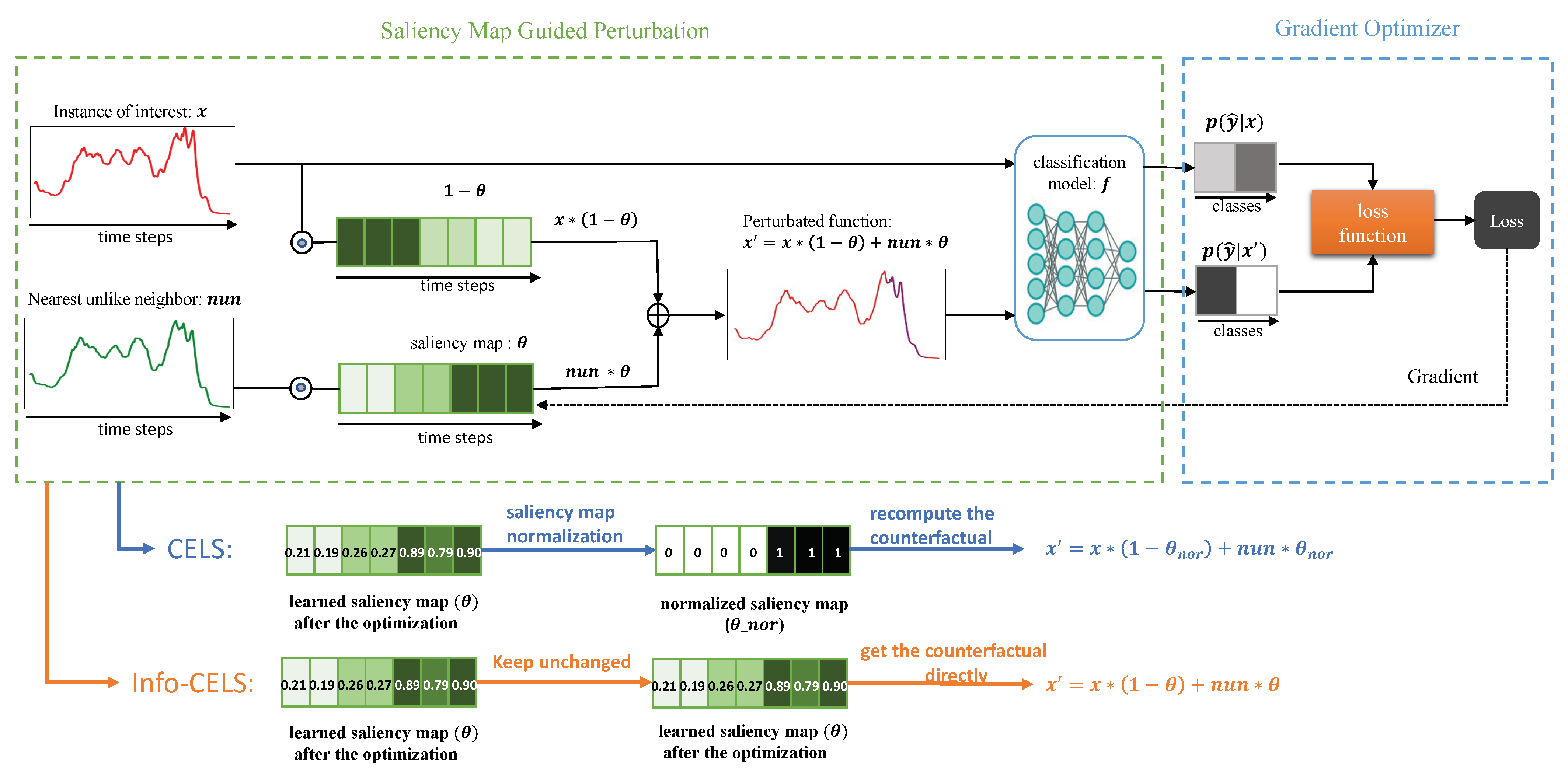
3.4. Counterfactual Perturbation

To learn an efficient saliency map, CELS proposes a perturbation function guided by the nearest unlike neighbor to assist in the saliency map-learning process. Equation (6) shows the perturbation function, where $nun$ is the reference sample used to guide the perturbation.

An element ${\mathit{\theta }}_t$ in $\mathit{\theta }$ represents the importance value of time steps t. Values of $\mathit{\theta }$ close to 1 indicate strong evidence supporting the prediction of class z, while values near 0 suggest that the corresponding time step is not important for the prediction of class z. Ideally, if ${\mathit{\theta }}_t=0$, it means that the time step t has no significant impact on the prediction, and the original value ${\mathbf{x}}_t$ at time step t remains unchanged. Conversely, if ${\mathit{\theta }}_t=1$, the time step ${\mathbf{x}}_t$ plays a crucial role in the prediction, and ${\mathbf{x}}_t$ is replaced by the corresponding time step from the nearest unlike neighbor $nun$. For values of ${\mathit{\theta }}_t$ between 0 and 1, the perturbation represents an interpolation between $\mathbf{x}$ and $nun$, with higher values indicating a greater influence of $nun$, and lower values retaining more of $\mathbf{x}$.

$${\mathbf{x}}^{\prime }=\mathbf{x}\odot \left(1-\mathit{\theta }\right)+nun\odot \mathit{\theta }$$

(6)

4. Informative CELS (Info-CELS)

In the original CELS algorithm, a threshold-based normalization step is applied to the learned saliency map $\mathit{\theta }$ before generating the final counterfactual explanation ${\mathbf{x}}^{\prime }$ (see Algorithm 1, line 11). Specifically, after several optimization epochs, each element for each $\mathit{\theta }\left[i\right]$ is set to 1 if it exceeds the threshold k, and 0 otherwise. This binary saliency map then determines which time steps are perturbed (see Algorithm 1, line 12). The primary motivation behind this normalization was to reduce the amount of perturbation applied to the original query instance, thereby yielding counterfactual explanations with higher sparsity.

However, this threshold-based normalization can inadvertently introduce noise into the final counterfactual explanation. Because the learned saliency map is abruptly converted into a binary saliency map, certain time steps may experience disproportionately large or sudden changes (i.e., “jumps”) in their values. These jumps can mask the true model-driven rationale by introducing artificial discontinuities, reducing interpretability and potentially obscuring the local decision boundary of the classifier. Figure 2a,c illustrate these abrupt changes for instances from the GunPoint and ECG datasets, respectively, where the normalization process yields noisy, step-like patterns.

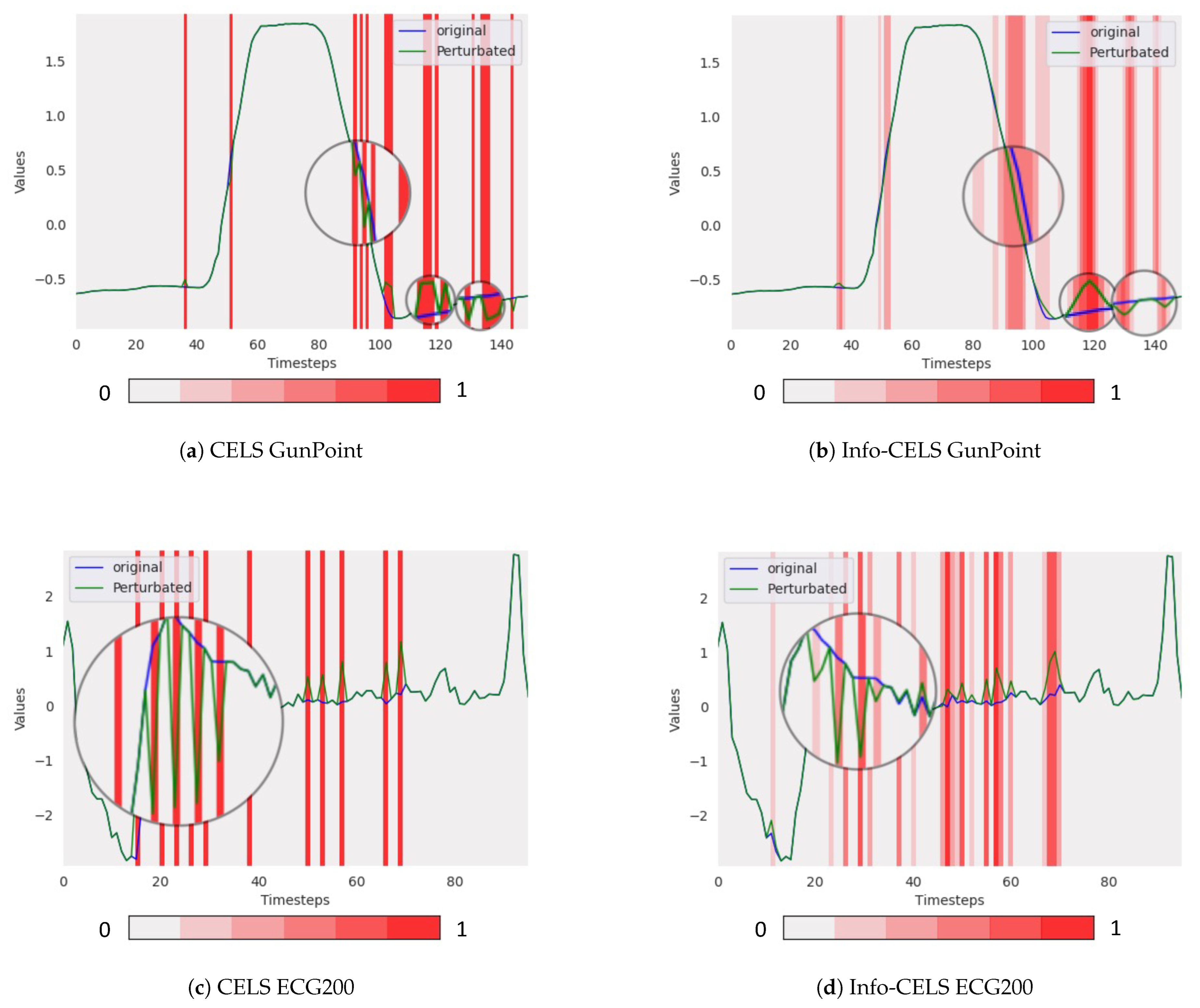
4.1. Detailed Analysis of Noise and Its Impact

To understand the nature of the noise introduced by normalization, it is helpful to examine how small variations in $\mathit{\theta }$ around the threshold k can lead to disproportionately large perturbations in the counterfactual instance ${\mathbf{x}}^{\prime }$. Some notable examples are as follows:

• Binary jumps: When $\mathit{\theta }\left[i\right]$ is near k, slight fluctuations during optimization can toggle the corresponding time step from 0 to 1 (or vice versa). This leads to sudden on/off behavior, creating sharp transitions in ${\mathbf{x}}^{\prime }$.
• Loss of Gradient Information: By converting $\mathit{\theta }\left[i\right]$ into a binary saliency map, the finer-grained information about how “important” a time step is (e.g., 0.2 vs. 0.8) is lost. The explanation can become less interpretable because partial saliency information is discarded.
• Reduced Smoothness: Counterfactuals often need to maintain temporal coherence—especially in time series—to be interpretable. The normalization step disrupts this coherence by enforcing large, piecewise-constant segments in ${\mathbf{x}}^{\prime }$.

As a result, the quality of the counterfactual explanation may reduce. The abrupt changes make it harder for domain experts to see meaningful patterns or transitions, and these sudden jumps can reduce confidence in the explanation’s trustworthiness.

4.2. Info-CELS: Noise Mitigation and Formal Rationale

To mitigate these issues, we introduce Info-CELS, which omits the threshold-based normalization (lines 12–13 in Algorithm 1). Instead, Info-CELS uses the learned saliency map $\mathit{\theta }$ directly to guide perturbations, allowing each time step to be perturbed proportionally to its importance rather than using a binary approach. Keeping the fractional saliency helps produce smoother changes in the perturbed instances and lowers the chance of sudden shifts.

• Noise Mitigation Strategy:
  • Smooth Perturbation: Because Info-CELS does not force $\mathit{\theta }\left[i\right]$ into binary values, time steps with moderate importance can be partially perturbed rather than entirely flipped on/off. This yields gradual transitions rather than sudden jumps.
  • Preservation of Fine-Grained Importance: The model’s local gradient information is preserved, as each time step’s saliency directly scales the magnitude of perturbation. This more closely aligns the counterfactual instance with the true local decision boundary.
• Formal Explanation of Improved Validity:
  • Faithfulness to the Learned Saliency: By using the continuous values of $\mathit{\theta }$, Info-CELS ensures that the counterfactual generation process remains consistent with the original optimization objective (i.e., finding the minimal perturbation needed to change the classification). This consistency avoids the abrupt, post-hoc distortion caused by thresholding.
  • Reduced Over-Correction: Threshold-based normalization can “over-correct” certain time steps, leading to out-of-bound or exaggerated perturbations. Eliminating the threshold reduces these extreme adjustments, increasing the likelihood that ${\mathbf{x}}^{\prime }$ will actually shift to the desired class (i.e., higher validity).
  • Smoother Decision Boundary Transitions: Many classifiers, especially those based on neural networks, respond more predictably to small, smooth perturbations than to abrupt, binary changes. Thus, Info-CELS produces counterfactuals that are more naturally positioned on the boundary between classes, improving the probability of valid classification.

4.3. Empirical Findings

In Figure 2, we compare the real examples of counterfactual explanations generated by CELS and Info-CELS. The results reveal that Info-CELS yields significantly smoother perturbations with fewer abrupt changes, thereby reducing noise and enhancing interpretability. Moreover, our experiments (Section 5.4) confirm that Info-CELS achieves 100% validity, maintaining comparable levels of sparsity and proximity to CELS. This indicates that removing the normalization step not only mitigates unnecessary noise but also improves the reliability of the counterfactual explanations by preserving the essential saliency information. Further details on the experimental evaluation are provided in Section 5.4.

In summary, Info-CELS directly addresses the drawbacks of threshold-based saliency map normalization in the following ways:

• Mitigating noise through smooth perturbations;
• Maintaining finer-grained saliency for interpretability;
• Ensuring high validity by avoiding abrupt, post-hoc changes that can distort the explanation’s fidelity.

5. Experiments

In this section, we provide a detailed description of our experimental design and discuss our findings. Our experiments were conducted using publicly available univariate time series datasets from the University of California, Riverside (UCR) Time Series Classification Archive [45]. Specifically, we selected seven widely-used real-world datasets from various domains, including Spectro, ECG, Motion, Simulated, Image, and Sensor. These datasets are known to demonstrate a high classification performance on state-of-the-art classifiers, as reported in [9], ensuring the quality of the counterfactual instances generated in our study. Additionally, these datasets are commonly used as benchmark datasets in recent research on counterfactual explanations for time series data [33,42,43]. The time series classes are evenly distributed across the training and testing partitions.

Table 1. UCR Datasets Metadata.

ID	Dataset Name	$\mathcal{C}$	$\mathcal{L}$	DS Train Size	DS Test Size	Type
0	Coffee	2	286	28	28	SPECTRO
1	GunPoint	2	150	50	150	MOTION
2	ECG200	2	96	100	100	ECG
3	TwoLeadECG	2	82	23	100	ECG
4	CBF	3	128	30	100	SIMULATED
5	BirdChicken	2	512	20	20	IMAGE
6	Plane	7	144	105	105	SENSOR

$\mathcal{C}$: number of classes; $\mathcal{L}$: time series length; DS: dataset.

provides the details of the datasets used. For the TwoLeadECG and CBF datasets, with original test set sizes of 1139 and 900, respectively, we randomly selected 100 samples from each test set to reduce computation time while still ensuring the counterfactual explanations were effectively learned.

5.1. Baseline Methods

We evaluated Info-CELS alongside CELS and four additional baselines—NG, Alibi, SG, and TimeX. These baselines were selected because they share a similar strategy of replacing key time steps or subsequences, either through heuristic methods or optimization-based approaches.

• Native guide counterfactual (NG): NG [42] is an instance-based counterfactual method that utilizes feature weight vectors and in-sample counterfactuals to generate counterfactuals. It extracts feature weight vectors using Class Activation Mapping (CAM) [46], which helps NG identify the most distinguishable contiguous subsequences. The nearest unlike neighbor is then used to replace these subsequences. To generate CAM, specific types of networks are typically required, particularly those that include convolutional layers or other feature extraction mechanisms capable of producing feature maps.
• Alibi Counterfactual (ALIBI): ALIBI follows the work of Wachter et al. [31], which generates counterfactual explanations by optimizing an objective function:

  $$\mathcal{L}={\mathcal{L}}_{pred}+{\mathcal{L}}_{L1},$$

  (7)

  where ${\mathcal{L}}_{pred}$ encourages the search of counterfactual instance to change the model prediction to the target class, and ${\mathcal{L}}_{L1}$ ensures that ${\mathbf{x}}^{\prime }$ is close to original instance $\mathbf{x}$. This method generates counterfactuals with only proximity and validity constraints on the perturbation, which could result in modifications across the entire time series to achieve the counterfactuals.
• Shapelet-guied counterfactual (SG): SG [33] is the extension based on wCF, which introduces a new shapelet loss term (see Equation (8)) to enforce the counterfactual instance ${\mathbf{x}}^{\prime }$ to be close to the promined shapelet ${\mathbf{x}}_{\mathbf{shapelet}}$ extracted from the training set. This method encourages one segment perturbation based on pre-mined shapelets. Using a brute force approach that compares all possible subsequences of various lengths in the time series could find the most discriminative shapelets, but it is computationally expensive. As a result, SG relies on the availability of high-quality extracted shapelets to guide counterfactual generation effectively. However, obtaining such high-quality shapelets is computationally costly, making the efficiency of SG heavily dependent on the extraction method used.

  $${\mathcal{L}}_{shapelet}=d({\mathbf{x}}^{\prime },{shapelet}_{z^{\prime }})$$

  (8)

  $$\mathcal{L}={\mathcal{L}}_{pred}+{\mathcal{L}}_{L1}+{\mathcal{L}}_{shapelet}$$

  (9)
• Time Series Counterfactual Explanations using Barycenters (TimeX): TimeX [35] builds upon Wachter’s counterfactual generation framework by introducing a new loss term that enhances interpretability and contiguity. It incorporates Dynamic Barycenter Averaging (DBA) [47] to ensure that the generated counterfactual is close to the average time series of the target class, thereby improving representativeness. Additionally, TimeX enforces contiguity by modifying only the most important contiguous segment, identified through saliency maps or perturbation-based evaluation. To ensure a valid counterfactual, the contiguous segment length is gradually increased until the perturbation is sufficient to change the classification, sometimes requiring a long subsequence modification.

  $${\mathcal{L}}_{dba}=d({\mathbf{x}}^{\prime }-db{a}_{z^{\prime }})$$

  (10)

  $$\mathcal{L}={\mathcal{L}}_{pred}+{\mathcal{L}}_{L1}+{\mathcal{L}}_{dba}$$

  (11)
• CELS [43]: An optimization-based model that generates counterfactual explanations by learning saliency maps to guide the perturbation. CELS is designed to identify and highlight the key time steps that provide crucial evidence for the model’s prediction. It achieves this by learning a saliency map for each input and using the nearest unlike neighbor as a reference to replace the important time steps identified by the saliency map.

5.2. Implementation Details

Each dataset from the UCR archive comes with a predefined training and testing set. We trained a Fully Convolutional Network (FCN) model on the training data to serve as a black-box classifier f, and generated counterfactuals for each sample in the test set. All baselines utilized the same model and test set to ensure fairness in the evaluation. We optimized Info-CELS using the ADAM optimizer [48] with an initial learning rate of 0.1 and trained for up to 1000 epochs. The optimization process includes early stopping based on convergence to prevent overfitting. Specifically, we monitored the loss function, and if the loss improvement fell below a defined threshold (imp_threshold = 0.001) for a specified number of iterations (max_iterations_without_improvement = 30), early stopping was triggered. We also applied exponential learning rate decay to improve convergence, with a decay factor defined by ‘gamma‘. The perturbation process involves optimizing the saliency map, a learnable variable that controls the modifications to the input. The saliency map was iteratively adjusted based on the gradients computed during backpropagation. The optimization continued until the target probability surpassed a threshold of 0.5 and early stopping conditions were met. The $\lambda$ we used in our experiments to balance the trade-off between validity and joint proximity and plausibility was set to 1 to ensure a high confidence level to obtain valid counterfactual explanations. To facilitate reproducibility and further exploration, we made our source code publicly available at (https://github.com/Luckilyeee/Info-CELS, accessed on 23 March 2025).

The source code for each baseline is publicly available: NG (https://github.com/e-delaney/Instance-Based_CFE_TSC, accessed on 23 March 2025), ALIBI (https://github.com/SeldonIO/alibi, accessed on 23 March 2025), TimeX (https://sites.google.com/view/timex-cf, accessed on 23 March 2025), SG-CF (https://github.com/Luckilyeee/SG-CF, accessed on 23 March 2025), and CELS (https://github.com/Luckilyeee/CELS, accessed on 23 March 2025). While generating counterfactuals for these baseline models, we use their original source code without modifying any parameters.

5.3. Evaluation Metrics

To evaluate our proposed method, we first compared Info-CELS with the other four baselines in terms of validity by evaluating the label flip rate for the prediction of the counterfactual explanation result and the target probability. We computed the flip rate following the formula of Equation (12).

$$flip\_rate={\displaystyle \frac{num\_flipped}{num\_testsample}},$$

(12)

where we denote the num_flipped as the number of generated counterfactual explanation samples that result in a different prediction label compared to the original input, and the num_test_samples is the total number of samples in the test dataset used to generate these counterfactual explanations. According to the validity property mentioned in Section 2.2, a counterfactual instance should result in a prediction that is different from the prediction of the original instance. Therefore, the flip rate directly aligns with this validity property by quantifying how often the generated counterfactual instances meet this criterion. A high flip rate 1 indicates that all the generated counterfactual instances are valid.

The target class probability measures the confidence level of the prediction for the counterfactual explanation. Specifically, it assesses how likely the model is to predict the counterfactual instance as belonging to the target class. The closer this probability is to 1, the more confident and desirable the prediction. This metric provides an additional layer of evaluation by not only ensuring that the counterfactual instances are valid (as measured by the flip rate) but also that they are predicted with high confidence. The results of these evaluations are presented in

Table 2. A comparison of the performances among different counterfactual explanation models in terms of flip rate and target probability (the winner is bolded).

	Flip Rate						Target Probability
Dataset	NG	ALIBI	SG	TimeX	CELS	Info-CELS	NG	ALIBI	SG	TimeX	CELS	Info-CELS
Coffee	1.0	0.79	0.61	1.0	0.786	1.0	0.67	0.74	0.60	0.96	0.62	0.9
GunPoint	1.0	0.95	0.92	1.0	0.680	1.0	0.63	0.87	0.86	0.96	0.59	0.97
ECG200	1.0	0.88	0.93	0.98	0.820	1.0	0.79	0.82	0.93	0.97	0.68	0.86
TwoLeadECG	1.0	0.87	1.0	1.0	0.6	1.0	0.80	0.83	0.99	0.98	0.57	0.84
CBF	0.56	0.89	0.81	0.97	0.71	1.0	0.41	0.83	0.78	0.93	0.56	0.86
BirdChicken	1.0	1.0	0.85	0.7	0.5	1.0	0.63	0.81	0.80	0.69	0.53	0.96
Plane	0.14	0.69	0.87	1.0	0.57	1.0	0.16	0.67	0.85	0.97	0.4	0.81

.

Next, we compared the L1 distance and sparsity level to evaluate the proximity and sparsity. L1 distance is defined in Equation (13). It measures the closeness between the generated counterfactual ${\mathbf{x}}^{\prime }$ and the original instance of interest $\mathbf{x}$. A smaller L1 distance is preferred.

$$L1distance=\sum _{t=1}^T\left(\right|{\mathbf{x}}_{\mathbf{t}}-{\mathbf{x}}_t^{\prime }\left|\right),$$

(13)

For the sparsity level, the highest sparsity is an indicator that the number of time series data points perturbations made in $\mathbf{x}$ to achieve ${\mathbf{x}}^{\prime }$ is minimal. Therefore, a higher sparsity level is desirable. The equations designed by [35] are shown in Equations (14) and (15), where T represents the total number of time steps (length) of the time series data.

$$Sparsity=1-{\displaystyle \frac{{\sum }_{t=1}^{T}g({\mathbf{x}}_t^{\prime },{\mathbf{x}}_t)}{T}}$$

(14)

$$g(x,y)=\left\{\begin{array}{cc}1,\hfill & \mathrm{if}x\ne y\hfill \\ 0,\hfill & \mathrm{otherwise}\hfill \end{array}\right.$$

(15)

5.4. Evaluation Results

In this section, we present the experimental results of different models across various datasets. Each test sample serves as a query instance to generate a corresponding counterfactual. Validity is measured by the flip rate, which represents the percentage of test samples that achieve the desired outcome. For target probability, sparsity level, L1 distance, and OOD, we report the average values across all samples. These metrics are computed based on the final perturbation results to evaluate their validity, proximity, sparsity, and plausibility.

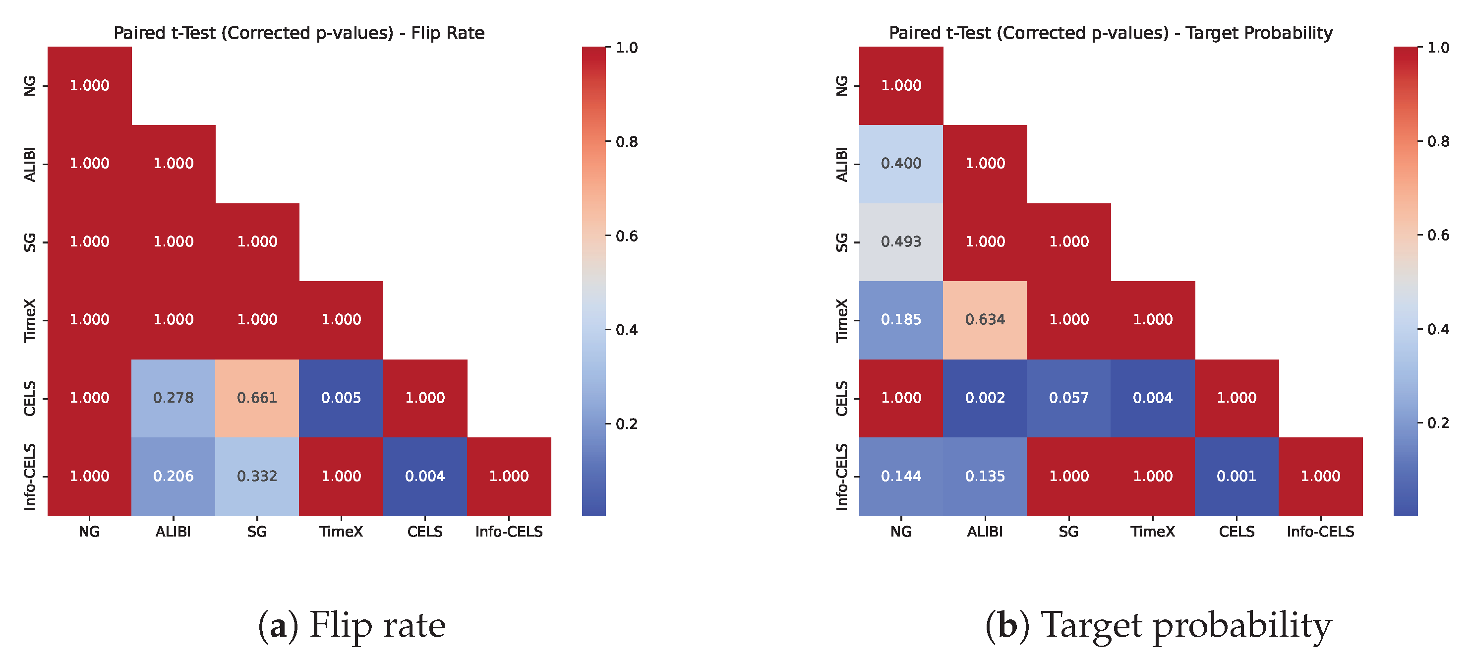
5.4.1. Validity Evaluation:

Table 2 shows the performance comparison of different counterfactual explanation models in terms of flip label rate and target probability. Based on the results in Table 2, Info-CELS consistently demonstrates a strong performance, achieving a stable 100% flip label rate with competitive target probability across various datasets. The lower flip rate of CELS is likely due to noise from saliency map normalization, as discussed in Section 4. While TimeX achieves a competitive target probability compared to other methods, it does not always guarantee 100% validity. This limitation may stem from its reliance on single subsequence replacement, which may not always provide a fully valid counterfactual. SG’s instability in validity may stem from the varying quality of selected shapelets. ALIBI’s global loss minimization can make finding optimal perturbations challenging. NG performs well in binary classification but struggles with multi-class cases, likely due to the quality of the class activation maps. To quantify the statistical significance of the pairwise differences in validity, Figure 3 presents heatmaps visualizing the corrected p-values from paired t-tests [49,50], comparing these methods. Notably, the paired t-tests confirmed the statistically significant improvement in both flip rate (p = 0.004) and target probability (p = 0.001) when comparing Info-CELS to CELS. While the t-tests did not indicate a statistically significant improvement over other baselines, Table 2 clearly shows that Info-CELS is the only method achieving 100% validity across all datasets. It is important to note that a p-value greater than 0.05 does not necessarily imply the absence of improvement; rather, it indicates that the observed difference may not be strong enough to rule out random variation with high confidence. In practical applications, achieving consistently 100% validity across diverse datasets is crucial, and the fact that Info-CELS outperforms all baselines in this regard suggests a meaningful advantage, even if the statistical test does not reach conventional significance thresholds.

The stable 100% flip label rate across various datasets achieved by Info-CELS indicates its effectiveness in generating counterfactual explanations that lead to changes in the predicted labels, thereby providing valuable insights into model behavior and decision-making processes. The stability of achieving a 100% validity rate across all datasets further underscores the reliability and consistency of our method in producing meaningful explanations.

Moreover, the consistently high target probability obtained by Info-CELS across all datasets, coupled with the significant t-test results when compared to CELS, highlights its ability to generate counterfactual explanations that are not only valid but also align closely with the desired outcomes. This implies that Info-CELS can offer valuable insights with a high confidence level into the decision-making process of complex machine learning models across diverse datasets, ultimately facilitating better understanding and trust in AI systems.

5.4.2. Sparsity and Proximity Evaluation:

Figure 4 shows our experimental results in terms of sparsity and proximity across different explanation models.

In Figure 4a, we show the comparison of sparsity property among the generated counterfactuals across various explanation models. The sparsity metric represents the percentage of data points that remain unchanged after perturbation. Our proposed Info-CELS model demonstrates significantly higher sparsity levels compared to ALIBI and achieves sparsity levels comparable to SG. Although Info-CELS demonstrates lower sparsity compared to CELS, TimeX, and NG, it is noteworthy that CELS, TimeX, and NG were unable to achieve 100% validity consistently across all datasets, indicating that some counterfactuals may not be valid due to insufficient perturbation. This suggests that while Info-CELS may compromise slightly on sparsity, it compensates for this by ensuring the validity of the generated counterfactual explanations, which is crucial for their usefulness and reliability in real-world applications.

Figure 4b evaluates the proximity property using the L1 distance metric. From this figure, we observe that Info-CELS achieves comparable proximity to the other baselines. Notably, Info-CELS stands out as the only model capable of generating counterfactuals with 100% validity. This is a significant advantage, as other baselines may generate counterfactual instances with lower L1 distances but fail to ensure their validity.

Overall, the results suggest that Info-CELS strikes a balance between validity and proximity, achieving a competitive performance while ensuring the validity of the generated counterfactual explanations. This highlights the effectiveness and reliability of Info-CELS in providing meaningful and trustworthy explanations for time series classification.

5.5. Exploring Interpretability (Also Referred to as Plausibility (e.g., [42]))

In Figure 2, we compare the perturbations obtained when applying CELS and Info-CELS. As mentioned, Info-CELS produces counterfactuals with smoother transitions and fewer abrupt changes, indicating reduced noise and enhanced interpretability. Building on this observation, we further explore the plausibility of the generated counterfactual explanations in time series data by employing novelty detection algorithms to detect out-of-distribution (OOD) explanations. Expanding on the concept of interpretability, as referenced in Section 2.2, we consider a counterfactual instance ${\mathbf{x}}^{\prime }$ interpretable if it closely resembles the distribution of the model’s training data. Specifically, ${\mathbf{x}}^{\prime }$ should be classified as an inlier with respect to the training dataset. By leveraging novelty detection algorithms to assess the plausibility of counterfactual explanations, we aim to ensure that the generated explanations are not only valid but are also realistic and trustworthy representations of potential alternative scenarios. Therefore, in this section, we implement the Isolation Forest (IF) [51], Local Outlier Factor Method (LOF) [52], and One-Class Support Vector Machine (OC-SVM) [53] to compare the plausibility of counterfactual explanations generated by CELS and Info-CELS.

• IF is an algorithm used for anomaly detection, which works on the principle of isolating observations. Unlike many other techniques that rely on a distance or density measure, Isolation Forest is based on the idea that anomalies are ‘few and different.’
• LOF is an algorithm used to identify density-based local outliers in a dataset. It works by comparing a point’s local density with its neighbors’ local densities to determine how isolated the point is.
• OC-SVM is a variant of the Support Vector Machine (SVM) used for anomaly detection. It is an unsupervised learning algorithm designed to identify data points that are significantly different from the majority of the data.

More experimental results for the other three baselines are shown on our project website (https://sites.google.com/view/infocelsts/home, accessed on 23 March 2025).

Table 3. Comparing the CELS and info-CELS models on plausibility using three OOD metrics (IF, LOF, OC-SVM). The results indicate the percentage of generated counterfactuals that are out-of-distribution (lower scores are better and the best are highlighted in bold).

	IF		LOF		OC-SVM
Dataset	CELS	Info-CELS	CELS	Info-CELS	CELS	Info-CELS
Coffee	0.34	0.318	0.036	0.036	0.143	0.107
GunPoint	0.214	0.175	0.267	0.22	0.073	0.047
ECG200	0.282	0.220	0.02	0.02	0.18	0.13
TwoLeadECG	0.381	0.362	0.02	0	0.22	0.22
CBF	0.159	0.074	0	0	0.75	0.38
BirdChicken	0.5	0.5	0.05	0.05	0.5	0.3
Plane	0.33	0.17	0.4	0.31	0.35	0.02

presents the percentage of generated counterfactuals that were identified as out-of-distribution instances. The results indicate that the percentage of out-of-distribution counterfactuals from Info-CELS is consistently lower than that from the CELS model. This finding suggests that the counterfactual explanations produced by Info-CELS are more plausible and align better with the underlying data distribution compared to those generated by CELS.

5.6. Parameter Analysis

Note that we used $\lambda =1$ in the previous experimental study section to ensure a high confidence level to obtain valid counterfactual explanations. In this section, we adopt the Coffee dataset to analyze the sensitivity of different $\lambda$ on the performance of validity, sparsity, proximity, and plausibility. Specifically, we apply $\lambda =\{0.1,0.2,0.3,0.4,0.5,0.6,0.7,0.8,0.9,1.0\}$ to Info-CELS to obtain the different counterfactuals on different $\lambda$ value settings. We then calculate the flip label rate, target probability, sparsity, L1 distance, and three OOD metrics(IF, LOF, OC-SVM) under the corresponding $\lambda$ value. Figure 5 shows the results of applying different $\lambda$ to Info-CELs.

From Figure 5a, we can see that when $\lambda =0.3$, we can already achieve 100% validity with a decent target probability of about 0.8. When we increase the $\lambda$ value, the target probability tends to increase continuously. Referring to Equation (2), ${\mathcal{L}}_{\mathrm{Max}}$ is directly proportional to $\lambda$, meaning that as $\lambda$ increases, the impact of ${\mathcal{L}}_{\mathrm{Max}}$ on the overall loss becomes more pronounced. Since ${\mathcal{L}}_{\mathrm{Max}}$ is designed to maximize the class probability of the predicted counterfactual class, a higher weight assigned to this loss component results in a stronger emphasis on achieving a higher target probability. Therefore, as $\lambda$ increases, the model prioritizes maximizing the class probability, leading to a steady increase in the target probability. However, the L1 distance also keeps increasing when $\lambda$ is increasing, which results in lower proximity. This trend occurs because the ${\mathcal{L}}_{\mathrm{Budget}}$ loss component in the total loss function Equation (5) becomes less influential with higher $\lambda$ values. As $\lambda$ increases, the weight assigned to ${\mathcal{L}}_{\mathrm{Budget}}$ becomes smaller relative to the ${\mathcal{L}}_{\mathrm{Max}}$ loss component. Consequently, the optimization process becomes less focused on minimizing the absolute values of $\mathit{\theta }$ to reduce the overall magnitude of saliency changes, which leads to a larger L1 distance. Thus, as $\lambda$ increases, the L1 distance tends to increase accordingly. Similarly, the decrease in sparsity can also be attributed to the same reason.

From Figure 5b, we can see that LOF is stable even when the $\lambda$ is changing and the OC-SVM also remains stable when $\lambda >0.3$. The overall trend of IF is decreasing while the $\lambda$ is increasing, IF achieves the lowest value when $\lambda =0.7$, and remains stable, with a slight increase, after $\lambda >0.7$.

Overall, these results illustrate the trade-offs inherent in adjusting $\lambda$. While a higher $\lambda$ improves the target probability, it may also lead to reduced proximity and sparsity. We selected $\lambda =1$ for the main experiments because it provides a more robust target probability even though it results in a slightly higher L1 distance. This choice reflects our emphasis on ensuring valid and reliable counterfactual explanations, where achieving a high target probability is critical.

6. Computational Impact

In this section, we compare the computational costs of our proposed Info-CELS method with those of other state-of-the-art approaches (CELS, Alibi, NG, SG, and TimeX). The evaluation considers two main aspects: (i) preparation time and (ii) counterfactual generation time.

6.1. Preparation Time

• NG: NG requires extracting feature vectors to locate the most distinguishable subsequences. This is typically achieved by computing Class Activation Maps (CAM) from the intermediate layers of a convolutional neural network. Consequently, a neural network must be trained to obtain these feature maps. If the black-box model is not based on convolutional architectures, alternative methods or modifications are needed to extract analogous features, potentially increasing both the computational cost and the complexity of the counterfactual generation process.
• SG: SG involves an extra step of extracting pre-mined shapelets from the training set, which can be computationally expensive. In this process, the shapelet transform algorithm is applied, as described in [33], where both the number of candidate shapelets and their lengths are defined by a set of window sizes. Specifically, for a time series of length T and k different window sizes, roughly $kT$ candidate shapelets are generated per series. For each candidate shapelet, the algorithm computes distances to all possible subsequences in the dataset using a sliding window with a step size of 1. This distance computation takes about $O(N·T)$ per candidate for N time series. Consequently, for a single time series, the cost for all candidate shapelets is approximately $O(kT·(N·T))=O(k·N·T^2)$, and for the entire dataset of N time series, the overall worst-case time complexity becomes $O(k·N^2·T^2)$. Additionally, the removal of similar shapelets involves sorting and pairwise comparisons of the candidate set, which further increases the computational cost.
• TimeX: TimeX uses dynamic barycenter averaging to ensure that the generated counterfactual is close to the target class average. The dynamic barycenter extraction adds extra overhead, similarly to the cost observed in shapelet extraction, albeit with a different algorithmic complexity. The dynamic barycenter averaging method extracts a representative time series (barycenter) by aligning each time series to the current barycenter using DTW and then updating the barycenter as the weighted average of the aligned points. The main computational cost is derived through computing the DTW paths for each time series, which takes about $O(T\times B)$ per series, where T is the time series length and B is the barycenter length. With N time series and a maximum of max_iter iterations, the overall cost is roughly $O(\text{max\_iter}\times N\times T\times B)$.
• Alibi and CELS: Both methods (Alibi and CELS) do not require additional preparatory steps. In CELS, a saliency map is learned via optimization and is directly integrated into the counterfactual generation process. This eliminates the need for separate feature extraction or subsequence selection procedures, resulting in lower preparation times compared to methods like NG, SG, and TimeX.

6.2. Counterfactual Generation Time

• NG: NG does not involve an optimization process; instead, it extends the subsequence until a valid counterfactual is found; therefore, its generation time is typically very fast if the feature weights vectors are available.
• Alibi, SG, and TimeX: These methods perturb the original time series and optimize a loss function. SG and TimeX incorporate predefined or dynamically determined subsequence positions (via pre-mined shapelets or dynamic barycenter averaging, respectively) to guide the perturbations. Such constraints can accelerate convergence relative to pure optimization, although the overall generation time may still be impacted by the extra preparatory overhead.
• CELS and Info-CELS: Both approaches learn a saliency map from scratch during the optimization process, which generally requires more time to converge compared to methods that use predefined locations to guide the perturbation. However, Info-CELS eliminates the threshold-based normalization step used in CELS. This reduction in processing overhead makes Info-CELS computationally more efficient than CELS, although both are optimization-based.

While NG offers the fastest counterfactual generation due to its non-optimization approach, its preparatory feature extraction can add some overhead. In contrast, SG and TimeX incur additional computational costs during preparation due to shapelet and barycenter extraction, respectively. Although Alibi, CELS, and Info-CELS are more efficient in preparation, the optimization process in CELS and Info-CELS is inherently more time-consuming due to the saliency map-learning. The elimination of the normalization step in Info-CELS provides a computational advantage over CELS, making it a more efficient option among the saliency-based methods. This balanced analysis highlights the trade-offs between preparation and generation times across different counterfactual explanation methods.

7. Case Study: Multivariate Time Series Data

To evaluate the impact of eliminating the normalization step in Info-CELS on multivariate data and tasks beyond univariate time series classification, we conducted a case study on two multivariate datasets (BasicMotions and Cricket) from the Human Activity Recognition (HAR) domain. HAR is the problem of predicting an activity (the class value) based on accelerometer and/or gyroscope data. These two datasets are publicly available multivariate time series datasets sourced from the University of East Anglia (UEA) MTS archive [54]. Each sample in these two datasets consists of time series with multiple dimensions, providing a more challenging scenario for generating counterfactual explanations.

7.1. Datasets

BasicMotion Dataset: The dataset was created during a student project in 2016, in which four students wore a smartwatch while performing four distinct activities. The smartwatch recorded both 3D accelerometer and 3D gyroscope data. The dataset is categorized into four classes: standing, walking, running, and playing badminton. Each participant performed each activity five times, with data sampled at 10 Hz over a ten-second interval.

Cricket Dataset: Cricket relies on umpires to communicate different game events to a remote scorer through specific hand signals. For example, a No-Ball is indicated by touching each shoulder with the opposite hand, while a TVReplay—a request for a video review—is signaled by miming the outline of a TV screen. The dataset introduced in Ko et al. [55] comprises four umpires performing twelve distinct signals, each repeated ten times. Data were recorded at 184 Hz using accelerometers attached to the umpires’ wrists, with each device capturing synchronous measurements along three axes (x, y, and z).

7.2. Experimental Results

In this section, we present a concise discussion of our findings on multivariate time series data using the BasicMotions and Cricket datasets. We adapted Info-CELS to learn a 2D saliency map for each multi-variate time series data and compared its performance (without normalization) with CELS (with normalization). Our goal was to see if removing the normalization step—which showed benefits in univariate cases—would similarly help in multivariate settings.

• BasicMotions: Both Info-CELS and CELS achieved a 100% flip rate on the BasicMotions dataset. Info-CELS attained a slightly higher average target probability (0.8935 vs. 0.8807), suggesting marginal gains in confidence. Figure 6a,b display the counterfactual explanations from CELS and Info-CELS on one randomly selected sample from the BasicMotions testing dataset—this sample was chosen at random since all samples successfully flipped the label. Figure 6a,b show that the time series dimensions for BasicMotions are relatively simple, and normalization does not appear to introduce significant noise or abrupt changes. Consequently, eliminating the normalization step offers only a small improvement in performance.
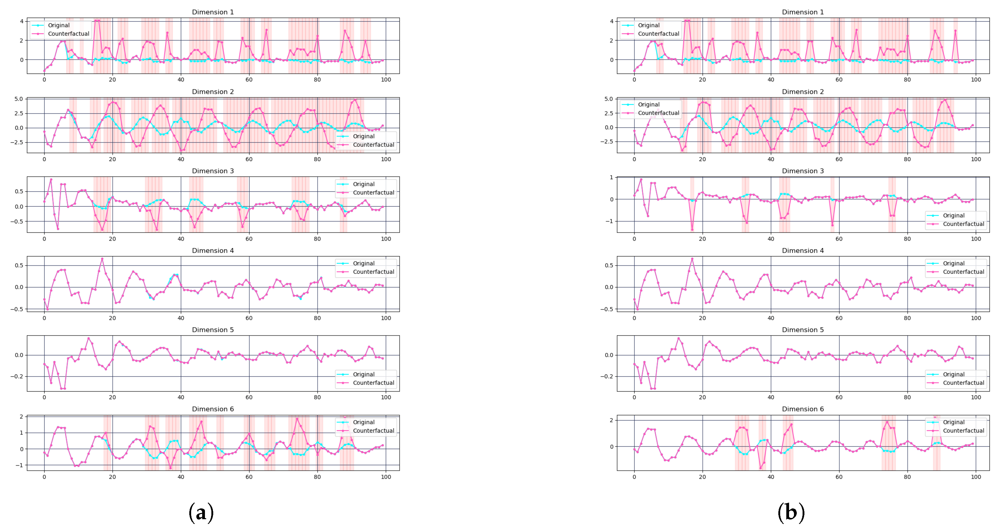
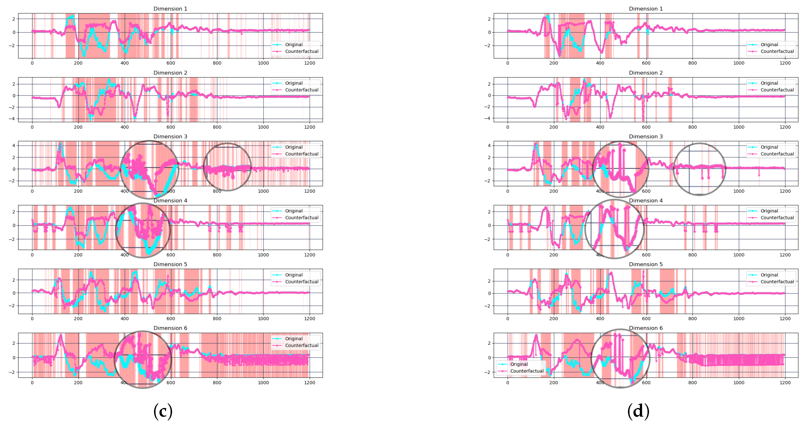
• Cricket: In contrast, Cricket benefits more noticeably from removing normalization. Info-CELS achieves a 100% flip rate, surpassing CELS (94.44%), and also exhibits a higher average target probability (0.8178 vs. 0.7597). Figure 6c,d focus on a Cricket instance that CELS failed to flip. We compared the original CELS explanation with Info-CELS on the same instance. As illustrated in Figure 6c,d, the signals in Cricket were more complex with higher variability across dimensions. Here, threshold-based normalization can cause abrupt, piecewise-constant segments in some channels, potentially undermining their validity. By maintaining continuous saliency values, Info-CELS avoids these artificial jumps, resulting in smoother perturbations and better classification flips.

Overall, these results show that while BasicMotions experiences only small improvements from removing normalization, datasets with more complex, multi-dimensional signals—such as Cricket—benefit significantly. This suggests that the effectiveness of omitting the normalization step is especially pronounced in multivariate settings with richer variability. Future work will extend this analysis to additional datasets and diverse application domains to further validate and refine the approach.

8. Conclusions

In this work, we introduced Info-CELS, a counterfactual explanation framework for time series classification that builds on and improves the original CELS model. The key innovation in Info-CELS is the removal of the threshold-based normalization of the learned saliency map. By preserving continuous saliency values, Info-CELS generates smoother and more informative perturbations, which in turn leads to a significant improvement in counterfactual validity. Our extensive experiments across multiple datasets demonstrate that Info-CELS consistently achieves 100% validity while maintaining competitive sparsity and proximity.

Overall, our contributions are threefold:

• We propose a novel modification to the CELS framework by eliminating the normalization step, thereby mitigating noise and enhancing the interpretability of counterfactuals.
• We provide a comprehensive empirical evaluation, demonstrating that Info-CELS achieves perfect validity and improved target probabilities across diverse datasets.
• We extend our investigation to multivariate time series data, highlighting their broader applicability in complex real-world scenarios.

These contributions not only advance the state-of-the-art in counterfactual explanations for time series data but also pave the way for future research on developing explainable AI systems that can operate reliably across varied data modalities.

References

1. Kaushik, S.; Choudhury, A.; Sheron, P.K.; Dasgupta, N.; Natarajan, S.; Pickett, L.A.; Dutt, V. AI in healthcare: Time-series forecasting using statistical, neural, and ensemble architectures. Front. Big Data 2020, 3, 4. [Google Scholar] [CrossRef] [PubMed]
2. Wang, W.K.; Chen, I.; Hershkovich, L.; Yang, J.; Shetty, A.; Singh, G.; Jiang, Y.; Kotla, A.; Shang, J.Z.; Yerrabelli, R.; et al. A systematic review of time series classification techniques used in biomedical applications. Sensors 2022, 22, 8016. [Google Scholar] [CrossRef]
3. Chaovalitwongse, W.A.; Prokopyev, O.A.; Pardalos, P.M. Electroencephalogram (EEG) time series classification: Applications in epilepsy. Ann. Oper. Res. 2006, 148, 227–250. [Google Scholar]
4. Mehdiyev, N.; Lahann, J.; Emrich, A.; Enke, D.; Fettke, P.; Loos, P. Time series classification using deep learning for process planning: A case from the process industry. Procedia Comput. Sci. 2017, 114, 242–249. [Google Scholar]
5. Susto, G.A.; Cenedese, A.; Terzi, M. Time-series classification methods: Review and applications to power systems data. Big Data Appl. Power Syst. 2018, 179–220. [Google Scholar] [CrossRef]
6. Hosseinzadeh, P.; Boubrahimi, S.F.; Hamdi, S.M. An End-to-end Ensemble Machine Learning Approach for Predicting High-impact Solar Energetic Particle Events Using Multimodal Data. Astrophys. J. Suppl. Ser. 2025, 277, 34. [Google Scholar]
7. Bahri, O.; Boubrahimi, S.F.; Hamdi, S.M. Shapelet-Based Counterfactual Explanations for Multivariate Time Series. arXiv 2022, arXiv:2208.10462. [Google Scholar]
8. Li, P.; Bahri, O.; Boubrahimi, S.F.; Hamdi, S.M. Fast Counterfactual Explanation for Solar Flare Prediction. In Proceedings of the 2022 21st IEEE International Conference on Machine Learning and Applications (ICMLA), Nassau, Bahamas, 12–14 December 2022; IEEE: Piscataway, NJ, USA, 2022; pp. 1238–1243. [Google Scholar]
9. Ismail Fawaz, H.; Forestier, G.; Weber, J.; Idoumghar, L.; Muller, P.A. Deep learning for time series classification: A review. Data Min. Knowl. Discov. 2019, 33, 917–963. [Google Scholar]
10. Liu, C.L.; Hsaio, W.H.; Tu, Y.C. Time series classification with multivariate convolutional neural network. IEEE Trans. Ind. Electron. 2018, 66, 4788–4797. [Google Scholar]
11. Fawaz, H.I.; Forestier, G.; Weber, J.; Idoumghar, L.; Muller, P.A. Deep neural network ensembles for time series classification. In Proceedings of the 2019 International Joint Conference on Neural Networks (IJCNN), Budapest, Hungary, 14–19 July 2019; IEEE: Piscataway, NJ, USA, 2019; pp. 1–6. [Google Scholar]
12. Zheng, Y.; Liu, Q.; Chen, E.; Ge, Y.; Zhao, J.L. Time series classification using multi-channels deep convolutional neural networks. In Proceedings of the International Conference on Web-Age Information Management, Macau, China, 16–18 June 2014; Springer: Berlin/Heidelberg, Germany, 2014; pp. 298–310. [Google Scholar]
13. Gamboa, J.C.B. Deep learning for time-series analysis. arXiv 2017, arXiv:1701.01887. [Google Scholar]
14. Adadi, A.; Berrada, M. Peeking inside the black-box: A survey on explainable artificial intelligence (XAI). IEEE Access 2018, 6, 52138–52160. [Google Scholar] [CrossRef]
15. Tjoa, E.; Guan, C. A survey on explainable artificial intelligence (xai): Toward medical xai. IEEE Trans. Neural Netw. Learn. Syst. 2020, 32, 4793–4813. [Google Scholar] [CrossRef] [PubMed]
16. Dwivedi, R.; Dave, D.; Naik, H.; Singhal, S.; Omer, R.; Patel, P.; Qian, B.; Wen, Z.; Shah, T.; Morgan, G.; et al. Explainable AI (XAI): Core ideas, techniques, and solutions. ACM Comput. Surv. 2023, 55, 1–33. [Google Scholar]
17. Arrieta, A.B.; Díaz-Rodríguez, N.; Del Ser, J.; Bennetot, A.; Tabik, S.; Barbado, A.; García, S.; Gil-López, S.; Molina, D.; Benjamins, R.; et al. Explainable Artificial Intelligence (XAI): Concepts, taxonomies, opportunities and challenges toward responsible AI. Inf. Fusion 2020, 58, 82–115. [Google Scholar] [CrossRef]
18. Van der Velden, B.H.; Kuijf, H.J.; Gilhuijs, K.G.; Viergever, M.A. Explainable artificial intelligence (XAI) in deep learning-based medical image analysis. Med Image Anal. 2022, 79, 102470. [Google Scholar] [CrossRef] [PubMed]
19. Saeed, W.; Omlin, C. Explainable AI (XAI): A systematic meta-survey of current challenges and future opportunities. Knowl.-Based Syst. 2023, 263, 110273. [Google Scholar] [CrossRef]
20. Nemirovsky, D.; Thiebaut, N.; Xu, Y.; Gupta, A. Countergan: Generating counterfactuals for real-time recourse and interpretability using residual gans. In Proceedings of the Uncertainty in Artificial Intelligence, Eindhoven, The Netherlands, 1–5 August 2022; PMLR: Birmingham, UK, 2022; pp. 1488–1497. [Google Scholar]
21. Brughmans, D.; Leyman, P.; Martens, D. Nice: An algorithm for nearest instance counterfactual explanations. Data Min. Knowl. Discov. 2024, 38, 2665–2703. [Google Scholar]
22. Dandl, S.; Molnar, C.; Binder, M.; Bischl, B. Multi-objective counterfactual explanations. In Proceedings of the International Conference on Parallel Problem Solving from Nature, Leiden, The Netherlands, 5–9 September 2020; Springer: Berlin/Heidelberg, Germany, 2020; pp. 448–469. [Google Scholar]
23. Rojat, T.; Puget, R.; Filliat, D.; Del Ser, J.; Gelin, R.; Díaz-Rodríguez, N. Explainable artificial intelligence (xai) on timeseries data: A survey. arXiv 2021, arXiv:2104.00950. [Google Scholar]
24. Bodria, F.; Giannotti, F.; Guidotti, R.; Naretto, F.; Pedreschi, D.; Rinzivillo, S. Benchmarking and survey of explanation methods for black box models. Data Min. Knowl. Discov. 2023, 37, 1719–1778. [Google Scholar] [CrossRef]
25. Ribeiro, M.T.; Singh, S.; Guestrin, C. “Why should i trust you?” Explaining the predictions of any classifier. In Proceedings of the 22nd ACM SIGKDD International Conference on Knowledge Discovery and Data Mining, San Francisco, CA, USA, 13–17 August 2016; pp. 1135–1144. [Google Scholar]
26. Lundberg, S.M.; Lee, S.I. A unified approach to interpreting model predictions. Adv. Neural Inf. Process. Syst. 2017, 30, 4768–4777. [Google Scholar]
27. Mahendran, A.; Vedaldi, A. Understanding deep image representations by inverting them. In Proceedings of the IEEE Conference on Computer Vision and Pattern Recognition, Boston, MA, USA, 7–12 June 2015; pp. 5188–5196. [Google Scholar]
28. Miller, T. Explanation in artificial intelligence: Insights from the social sciences. Artif. Intell. 2019, 267, 1–38. [Google Scholar]
29. Verma, S.; Boonsanong, V.; Hoang, M.; Hines, K.; Dickerson, J.; Shah, C. Counterfactual explanations and algorithmic recourses for machine learning: A review. ACM Comput. Surv. 2024, 56, 1–42. [Google Scholar]
30. Lee, M.H.; Chew, C.J. Understanding the effect of counterfactual explanations on trust and reliance on ai for human-ai collaborative clinical decision making. Proc. ACM Human-Comput. Interact. 2023, 7, 1–22. [Google Scholar]
31. Wachter, S.; Mittelstadt, B.; Russell, C. Counterfactual explanations without opening the black box: Automated decisions and the GDPR. Harv. JL Tech. 2017, 31, 841. [Google Scholar]
32. Li, P.; Boubrahimi, S.F.; Hamd, S.M. Motif-guided Time Series Counterfactual Explanations. arXiv 2022, arXiv:2211.04411. [Google Scholar]
33. Li, P.; Bahri, O.; Boubrahimi, S.F.; Hamdi, S.M. SG-CF: Shapelet-Guided Counterfactual Explanation for Time Series Classification. In Proceedings of the 2022 IEEE International Conference on Big Data (Big Data), Osaka, Japan, 17–20 December 2022; IEEE: Piscataway, NJ, USA, 2022; pp. 1564–1569. [Google Scholar]
34. Bahri, O.; Li, P.; Boubrahimi, S.F.; Hamdi, S.M. Temporal Rule-Based Counterfactual Explanations for Multivariate Time Series. In Proceedings of the 2022 21st IEEE International Conference on Machine Learning and Applications (ICMLA), Nassau, Bahamas, 12–14 December 2022; IEEE: Piscataway, NJ, USA, 2022; pp. 1244–1249. [Google Scholar]
35. Filali Boubrahimi, S.; Hamdi, S.M. On the Mining of Time Series Data Counterfactual Explanations using Barycenters. In Proceedings of the 31st ACM International Conference on Information & Knowledge Management, Atlanta, GA, USA, 17–21 October 2022; pp. 3943–3947. [Google Scholar]
36. Wang, Z.; Samsten, I.; Miliou, I.; Mochaourab, R.; Papapetrou, P. Glacier: Guided locally constrained counterfactual explanations for time series classification. Mach. Learn. 2024, 113, 4639–4669. [Google Scholar]
37. Sivill, T.; Flach, P. Limesegment: Meaningful, realistic time series explanations. In Proceedings of the International Conference on Artificial Intelligence and Statistics, Virtual, 28–30 March 2022; PMLR: Birmingham, UK, 2022; pp. 3418–3433. [Google Scholar]
38. Huang, Q.; Kitharidis, S.; Bäck, T.; van Stein, N. TX-Gen: Multi-Objective Optimization for Sparse Counterfactual Explanations for Time-Series Classification. arXiv 2024, arXiv:2409.09461. [Google Scholar]
39. Refoyo, M.; Luengo, D. Sub-SpaCE: Subsequence-Based Sparse Counterfactual Explanations for Time Series Classification Problems. 2023. Available online: https://www.researchsquare.com/article/rs-3706710/v1 (accessed on 23 March 2025).
40. Refoyo, M.; Luengo, D. Multi-SpaCE: Multi-Objective Subsequence-based Sparse Counterfactual Explanations for Multivariate Time Series Classification. arXiv 2024, arXiv:2501.04009. [Google Scholar]
41. Höllig, J.; Kulbach, C.; Thoma, S. TSEvo: Evolutionary Counterfactual Explanations for Time Series Classification. In Proceedings of the 21st IEEE International Conference on Machine Learning and Applications, ICMLA, Nassau, Bahamas, 12–14 December 2022; pp. 29–36. [Google Scholar] [CrossRef]
42. Delaney, E.; Greene, D.; Keane, M.T. Instance-based counterfactual explanations for time series classification. In Proceedings of the International Conference on Case-Based Reasoning, Salamanca, Spain, 13–16 September 2021; Springer: Berlin/Heidelberg, Germany, 2021; pp. 32–47. [Google Scholar]
43. Li, P.; Bahri, O.; Boubrahimi, S.F.; Hamdi, S.M. CELS: Counterfactual Explanations for Time Series Data via Learned Saliency Maps. In Proceedings of the 2023 IEEE International Conference on Big Data (BigData), Sorrento, Italy, 15–18 December 2023; IEEE: Piscataway, NJ, USA, 2023; pp. 718–727. [Google Scholar]
44. Mothilal, R.K.; Sharma, A.; Tan, C. Explaining machine learning classifiers through diverse counterfactual explanations. In Proceedings of the 2020 Conference on Fairness, Accountability, and Transparency, Barcelona, Spain, 27–30 January 2020; pp. 607–617. [Google Scholar]
45. Dau, H.A.; Bagnall, A.; Kamgar, K.; Yeh, C.C.M.; Zhu, Y.; Gharghabi, S.; Ratanamahatana, C.A.; Keogh, E. The UCR time series archive. IEEE/CAA J. Autom. Sin. 2019, 6, 1293–1305. [Google Scholar]
46. Zhou, B.; Khosla, A.; Lapedriza, A.; Oliva, A.; Torralba, A. Learning deep features for discriminative localization. In Proceedings of the IEEE Conference on Computer Vision and Pattern Recognition, Las Vegas, NV, USA, 27–30 June 2016; pp. 2921–2929. [Google Scholar]
47. Petitjean, F.; Ketterlin, A.; Gançarski, P. A global averaging method for dynamic time warping, with applications to clustering. Pattern Recognit. 2011, 44, 678–693. [Google Scholar]
48. Kingma, D.P.; Ba, J. Adam: A method for stochastic optimization. arXiv 2014, arXiv:1412.6980. [Google Scholar]
49. Student. The probable error of a mean. Biometrika 1908, 6, 1–25. [Google Scholar]
50. Moore, D.S.; McCabe, G.P.; Craig, B.A. Introduction to the Practice of Statistics; WH Freeman: New York, NY, USA, 2009; Volume 4. [Google Scholar]
51. Liu, F.T.; Ting, K.M.; Zhou, Z.H. Isolation forest. In Proceedings of the 2008 Eighth IEEE International Conference on Data Mining, Pisa, Italy, 15–19 December 2008; IEEE: Piscataway, NJ, USA, 2008; pp. 413–422. [Google Scholar]
52. Breunig, M.M.; Kriegel, H.P.; Ng, R.T.; Sander, J. LOF: Identifying density-based local outliers. In Proceedings of the 2000 ACM SIGMOD International Conference on Management of Data, Dallas, TX, USA, 15–18 May 2000; pp. 93–104. [Google Scholar]
53. Schölkopf, B.; Platt, J.C.; Shawe-Taylor, J.; Smola, A.J.; Williamson, R.C. Estimating the support of a high-dimensional distribution. Neural Comput. 2001, 13, 1443–1471. [Google Scholar] [PubMed]
54. Bagnall, A.; Dau, H.A.; Lines, J.; Flynn, M.; Large, J.; Bostrom, A.; Southam, P.; Keogh, E. The UEA multivariate time series classification archive. arXiv 2018, arXiv:1811.00075. [Google Scholar]
55. Ko, M.H.; West, G.; Venkatesh, S.; Kumar, M. Online context recognition in multisensor systems using dynamic time warping. In Proceedings of the 2005 International Conference on Intelligent Sensors, Sensor Networks and Information Processing, Melbourne, Australia, 5–8 December 2005; IEEE: Piscataway, NJ, USA, 2005; pp. 283–288. [Google Scholar]
Figure 1. Counterfactual explanation for time series data via learned saliency maps.
Electronics 14 01311 g001
Figure 2. Counterfactual explanations obtained from CELS and Info-CELS for the ECG200 and GunPoint datasets. (The x-axis in each figure represents the time steps, indicating the progression of time in the time series data. The y-axis denotes the values corresponding to each time step, showing the changes in the data over time. Below the figure, the one-dimensional saliency map highlights the importance scores for each time step, ranging between 0 and 1. A score of 1 means the time step is most influential in the model’s decision-making process).
Electronics 14 01311 g002
Figure 3. Heatmaps of corrected p-values from paired t-tests comparing counterfactual explanation methods for (a) flip rate and (b) target probability. The lower triangle displays corrected p-values, with lower values indicating statistically significant differences. The p-values were corrected using Bonferroni correction.
Electronics 14 01311 g003
Figure 4. Sparsity (the higher the better) and L1 distance (the lower the better) comparison of the CF explanations generated by ALIBI, NG, SG, CELS, and Info-CELS (all the reported results are the average value for the counterfactual set).
Electronics 14 01311 g004
Figure 5. Parameter analysis on the Coffee dataset. The figure compares the effects of different λ values on the model’s performance.
Electronics 14 01311 g005
Figure 6. Counterfactual explanations for the BasicMotions and Cricket datasets with and without saliency map normalization. (a) BasicMotions (Info-CELS); (b) BasicMotions (CELS with saliency map normalization); (c) Cricket (Info-CELS); (d) Cricket (CELS with saliency map normalization).
Electronics 14 01311 g006aElectronics 14 01311 g006b