FAFedZO: Faster Zero-Order Adaptive Federated Learning Algorithm

Abstract

Federated learning represents a newly emerging methodology in the field of machine learning that enables distributed agents to collaboratively learn a centralized model without sharing their raw data. Some scholars have already proposed many first-order algorithms and second-order algorithms for federated learning to reduce communication costs and speed up convergence. However, these algorithms generally rely on gradient or Hessian information, and we find it difficult to solve such federated optimization problems when the analytical expression of the loss function is not available, that is, when gradient information is not available. Therefore, we employed derivative-free federated zero-order optimization in this paper, which does not rely on specific gradient information, but instead utilizes the changes in function values or model outputs to estimate the optimization direction. Furthermore, to enhance the performance of derivative-free zero-order optimization, we propose an effective adaptive algorithm that can dynamically adjust the learning rate and other hyperparameters based on the performance during the optimization process, aiming to accelerate convergence. We rigorously analyze the convergence of our approach, and the experimental findings demonstrate our method can indeed achieve faster convergence speed on the MNIST, CIFAR-10 and Fashion-MNIST datasets in cases where gradient information is not available.

1. Introduction

With the rapid development of big data and artificial intelligence technologies, machine learning has become one of the key technologies in various fields. However, in practical applications, issues of data privacy and security have become a non-negligible challenge. In traditional machine learning, data usually need to be sent to data centers for model training, but in the process of transmission, the problems of data leakage and privacy protection are faced. To address this issue, federated learning (FL) [1], an emerging distributed machine learning technology, has emerged. It achieves collaborative learning among multiple data sources while protecting data privacy by exchanging model parameters instead of raw data. Currently, FL is utilized across diverse domains such as autonomous driving [2], personalized recommendation systems [3], and medical informatics [4], among others.

In order to meet the requirements of various scenarios in real-world applications, a large number of corresponding algorithms for federated learning have been studied. In recent years, to achieve fast convergence rates and reduce communication loads, a wide range of algorithms have been proposed, and these algorithms are commonly divided into two categories. One category is first-order methods [1,5,6], which only rely on the first-order derivative (gradient) of the objective function. The gradient indicates the direction in which the function increases most rapidly, and this type of method uses this information to iteratively update the model parameters. The other category is second-order methods. This kind of method not only utilizes the first-order derivative but also makes use of the second-order derivative (Hessian matrix), such as Fed-Sophia [7]. Most of these algorithms rely on gradient or Hessian information, and their scope of application is usually limited to differentiable functions. However, when the objective function has difficulty computing gradients or the gradient computation cost is excessively high, these algorithms will not be able to solve such problems, such as in the case of black-box functions and in federated hyperparameter tuning [8], so we must look for other solutions.

Zero-order optimization is a method proposed to reduce the dependence on gradient or Hessian information for optimizing the objective function. Its characteristic is that it does not require the calculation of the gradient. Instead, it estimates the change of the function by sampling the objective function to find the optimal solution. Therefore, this method is applicable to cases where the objective function is non-differentiable or the gradient is difficult to calculate. However, existing zero-order methods lack the utilization of gradient and other related information, resulting in the need for more iterations to achieve convergence during the optimization process. This greatly increases the computational time and affects the performance and convergence speed of the model. In deep learning, an excessively large learning rate may lead to unstable model training, resulting in overfitting or underfitting. Furthermore, traditional fixed learning rate methods often struggle to adapt to complex and diverse training data and model structures, potentially leading to a slow convergence speed of the model. The emergence of adaptive methods has effectively alleviated the problem of slow convergence. The adaptive method can dynamically adjust the learning rate based on feedback from the training process, thereby accelerating the convergence of the model. In addition, compared with stochastic gradient descent, this method can also escape saddle points more quickly [9]. Therefore, introducing it in practice represents a crucial approach to enhancing the performance of federated learning algorithms.

However, the improper design of adaptive federated learning methods may lead to convergence issues [10]. In the context of federated learning, data distribution across different devices often does not follow the IID (Independent and Identically Distributed) assumption, which further complicates the convergence problem. Reddi et al. [11] first proposed a federated version of the adaptive optimizer, among which are FedAdagrad and FedYogi. However, their analysis is only valid under the condition that ${\beta }_1=0$, where ${\beta }_1$ is the decay parameter, which cannot leverage the advantages of momentum. And these limitations become even more pronounced when dealing with non-IID (Non-Independent and Identically Distributed) data. The algorithm FedCAMS [12] provides a complete proof, but it does not improve the convergence speed. Moreover, they usually require a global learning rate for initialization and adjustment, and the selection of this global learning rate may affect the performance of the algorithm. Existing adaptive methods still have shortcomings, such as a lagging response to complex environmental changes and a high consumption of computational resources. Our goal is to design adaptive algorithms tailored to various real-world scenarios, characterized by efficiency, precision, and flexibility, so as to rapidly adapt to environmental changes, optimize resource allocation, and provide robust support for development across various fields.

Based on the above, we combine the gradient-free optimization with adaptive methods, aiming to leverage the advantages of both to solve the problem of unavailable gradient information of the objective function in a finite-sum optimization problem while achieving fast convergence and effectively improving the training efficiency and performance of the model.

The contributions of this paper are summarized as follows:

• By combining the zero-order optimization and adaptive gradient method, we proposed a novel faster zero-order adaptive federated learning algorithm, called FAFedZO, which can eliminate the reliance on gradient information and accelerate convergence at the same time.
• We conducted a theoretical analysis of the proposed zero-order adaptive algorithm and provided a convergence analysis framework under some mild assumptions, demonstrating its convergence. Additionally, we have analyzed the computational complexity and convergence rate of the algorithm.
• We have conducted a large number of comparative experiments on the MNIST, CIFAR-10, and Fashion-MNIST datasets. The experimental results verify the effectiveness of the FAFedZO algorithm. Compared with traditional zero-order optimization algorithms, this algorithm demonstrates significant performance advantages in both IID and non-IID scenarios.

The structure of the rest of this paper is outlined below. Section 2 provides a summary of the related work. In Section 3, we present the formulation of the federated optimization problem and the algorithm framework of FAFedZO. Section 4 provides the convergence analysis of FAFedZO. Section 5 presents the outcomes of our experiments. The paper concludes with Section 6.

2. Related Work

2.1. Federated Learning

There have been numerous studies on federated learning. Just as in the flight control neural network [13], optimal feedback gains are obtained through the meticulous design of the network architecture and training, and federated learning is also seeking the optimal parameter combinations for each client to achieve better global model performance. The pioneering work on federated learning began with [1], which proposed an algorithm called FedAvg. After FedAvg, numerous additional first-order schemes emerged, such as FedNova [14], FedProx [15], SCAFFOLD [16], FedSplit [17], and FedPD [18]. Among them, SCAFFOLD employs control variates to rectify “client drift” while maintaining the same sampling and communication complexity as FedAvg. FedProx introduced a penalty-based approach, which can reduce communication complexity to $O\left({ϵ}^{-2}\right)$. To further minimize communication costs, various second-order optimization methods have been introduced, including GIANT [19] and FedDANE [20]. Additionally, there are also some FL algorithms based on momentum, including [21,22,23]. The work presented in [21] proposes a momentum fusion approach for synchronizing the server and local momentum buffers; however, it does not aim to decrease complexity. Ref. [22] proposed a momentum-based global update algorithm, Fed-GLOMO, which reduces variance on the server side using variance-reduction techniques. Ref. [23] proposed the STEM algorithm, which employs momentum-assisted stochastic gradient directions for updates at both the worker nodes and the central server. However, there are still numerous federated optimization problems in reality that are challenging to solve, for instance, when gradient information is unavailable or costly to acquire. Therefore, the study of gradient-free zero-order optimization is essential.

2.2. Zero-Order Optimization

Early literature that began to use the zero-order idea for estimation includes [24,25,26]. Specifically, in [24], the authors developed a distributed zero-order algorithm utilizing gradient tracking techniques. In [25], the author provides the first generalization error analysis for black-box learning via derivative-free optimization and demonstrates that under the assumption of Lipschitz and smoothing (unknown) losses, the ZoSS method attains a comparable generalization error boundary to stochastic gradient descent (SGD). Ref. [26] proposed and analyzed zero-order stochastic approximation algorithms for non-convex and convex objective functions, focusing on solving the problems of constrained optimization and high-dimensional settings. Recent key research achievements have also applied zero-order methods to various fields, such as [27,28,29,30]. In [27], a derivative-free algorithm, FedZO, is proposed. It is proven that this algorithm achieves a linear increase in speed in relation to the number of devices involved and local iteration times under non-convex settings. Ref. [28] proposed the FedDisco algorithm, leveraging zero-order optimization techniques to reduce communication overhead significantly. Ref. [29] designed a federated zero-order algorithm, FedZeN, which focused on convex optimization, and estimated the curvature of the global objective. Under the framework of cross-device federated learning, Ref. [30] introduces a dual-communication zero-order method, which is the first technique to incorporate wireless channels into the algorithm. This represents a significant new achievement in the field of zero-order optimization, achieving a convergence rate of $O\left({\displaystyle \frac{1}{\sqrt[3]{K}}}\right)$ in non-convex settings, where K represents the total number of iterations. However, due to the nature of zero-order optimization, it can lead to slower convergence speeds. Therefore, an adaptive method is introduced below.

2.3. Adaptive Methods

Early proposed adaptive algorithms include [31,32]. The Adam method in [31] introduces decay coefficients and combines momentum optimization to better adapt to non-stationary data and large-scale datasets, thereby accelerating model convergence. The AdaGrad method in [32] can adaptively adjust the learning rate of each parameter that can make sparse features obtain larger learning rates, while frequently occurring features obtain smaller learning rates. Then, researchers have extended these algorithms to the context of federated learning, like recent studies such as [33,34,35,36]. In [33], the authors designed an Adaptive Local Iteration Differential Privacy Federated Learning algorithm (ALI-DPFL) and demonstrated its superiority in resource-constrained scenarios. The adaptive methods in [34,35] effectively mitigate the issue of non-IID data, achieving critical progress in enabling better performance when dealing with non-IID data. Ref. [35] introduced a novel framework called FedARF, which adopted an adaptive feature fusion strategy, enabling the model to better adapt to the data distribution of each client, thereby accelerating the convergence speed on non-IID data. Ref. [36] introduced a novel federated learning algorithm named AFedAvg, which significantly reduced communication costs and accelerated convergence speed by combining adaptive communication frequency and gradient sparsity techniques. However, none of these studies have investigated the integration of adaptive methods within the context of zero-order optimization. Hence, our article addresses this by combining zero-order optimization with adaptive approaches to conduct our discussion.

3. Problem Formulation and Algorithm Design

In this section, we will introduce the federated optimization problem and the design of the zero-order adaptive federated optimization algorithm FAFedZO.

3.1. Federated Optimization Problem Formulation

We consider a federated learning task involving a central server and Q edge devices with an index of $\{1,2,\dots ,Q\}$. The central server aims to facilitate collaboration among these devices to address a specific optimization problem

$$\begin{array}{c}\hfill \underset{\mathbf{\Xi }\in R^d}{min}f(\mathbf{\Xi })\triangleq {\displaystyle \frac{1}{Q}}\sum _{i=1}^Q{f}_i(\mathbf{\Xi }),\end{array}$$

(1)

in which

$$\begin{array}{c}\hfill f_i(\mathbf{\Xi })\triangleq E_{{\vartheta }_i\sim D_i}\left[F_i(\mathbf{\Xi },{\vartheta }_i)\right],\end{array}$$

(2)

where $\mathbf{\Xi }\in R^d$ represents a d-dimensional model parameter. For each edge device $i\in \left[Q\right]$, $\left[Q\right]$ represents all Q edge devices from 1 to Q, $f_i(\mathbf{\Xi })$ denotes its local loss function, while $f(\mathbf{\Xi })$ stands for the global loss function. In Equation (1), $f_i(\mathbf{\Xi })$ evaluates the anticipated risk on the data distribution $D_i$ on the edge device i, which is presented in Equation (2). ${\vartheta }_i\sim D_i$ denotes that the random variable ${\vartheta }_i$ is uniformly drawn from the distribution $D_i$, and $F_i(\mathbf{\Xi },{\vartheta }_i)$ denotes the loss function of ${\vartheta }_i$ at the parameter $\mathbf{\Xi }$.

3.2. Algorithm Design of FAFedZO

We explored how to design a method that combines an adaptive gradient with zero-order optimization in federated learning.

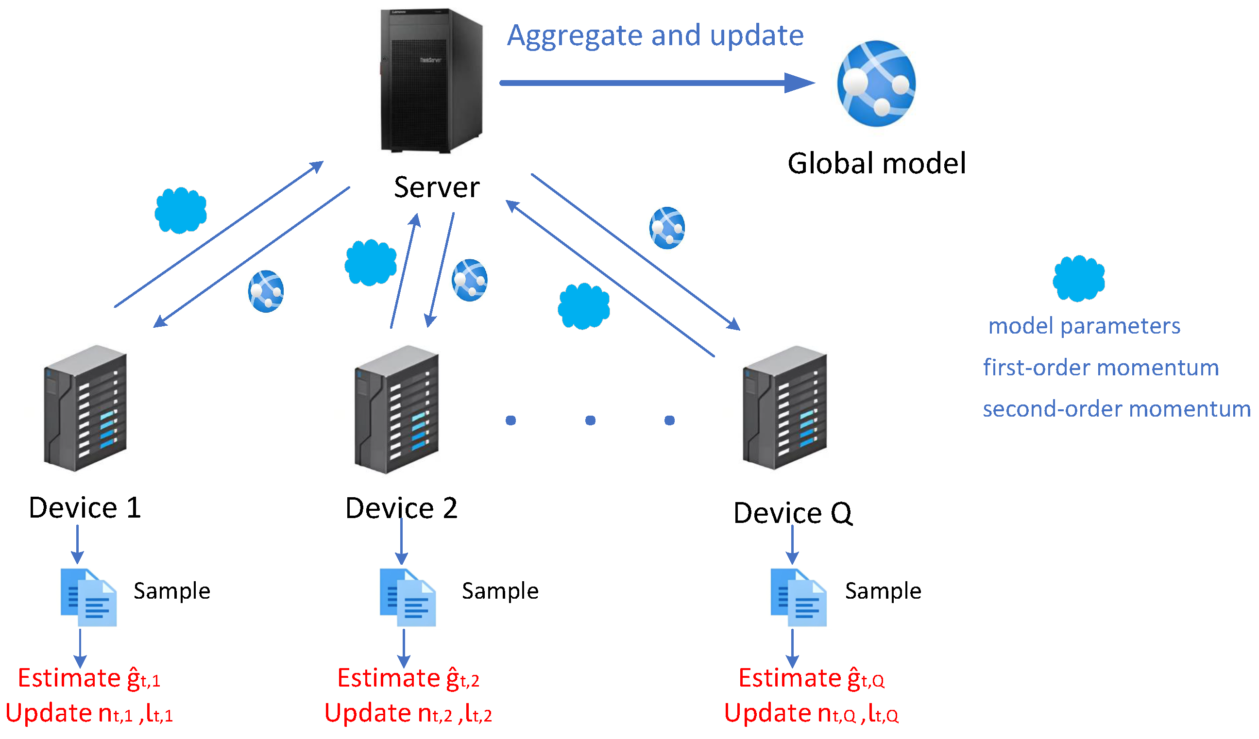
Firstly, we expand our algorithm description within the context of the FedAvg framework. We are focused here on solving problem (1) through zero-order optimization methods and propose a novel zero-order fast adaptive FL method (FAFedZO) that employs a shared adaptive learning rate. In particular, Algorithm 1 outlines the specifics of our FAFedZO method.

At the beginning, input the parameters and perform initialization. For all i, compute ${\mathbf{\Xi }}_{1,i}={\mathbf{\Xi }}_{0,i}-{\eta }_0{n}_{0,i}$, which represents the first model update based on the initial parameters and the initial gradient estimates.

Then, from round $t=1$ to T, perform the following: for each edge device $i\in \left[Q\right]$, first, extract a mini-batch ${\mathfrak{B}}_{t,i}$ of size b from the local dataset $D_i$. Next, compute the stochastic gradient estimates ${\widehat{g}}_{t,i}$ and ${\widehat{g}}_{t-1,i}$ for the current model parameters ${\mathbf{\Xi }}_{t,i}$ based on the mini-batch ${\mathfrak{B}}_{t,i}$. Here, we elaborate on the specific method for estimating the gradients.

To address the issue of unavailable gradient information and to reduce the frequency of model exchange, we use gradient estimators and perform stochastic zero-order updates in each communication round. By utilizing the gradient estimator, we can approximate the gradient through random sampling and estimation, without the need to precisely calculate the derivative of the function. In particular, at the t-th round, edge device i calculates a two-point stochastic gradient estimator [24], as outlined below

$$\begin{array}{c}\hfill {\tilde{\nabla }}_v^{\mu }{F}_i({\mathbf{\Xi }}_{t,i},{\vartheta }_{t,i})={\displaystyle \frac{d{\mathit{v}}_t}{{\mu }_t}}\left(F_i({\mathbf{\Xi }}_{t,i}+{\mu }_t{\mathit{v}}_t,{\vartheta }_{t,i})-F_i({\mathbf{\Xi }}_{t,i},{\vartheta }_{t,i})\right),\end{array}$$

(3)

where ${\mathbf{\Xi }}_{t,i}$ denotes the local model of edge device i, while ${\vartheta }_{t,i}$ signifies a random variable drawn by edge device i according to its local data distribution $D_i$ during the t-th round. ${\mathit{v}}_t$ represents a randomly chosen d-dimensional direction, uniformly sampled from the unit sphere ${\mathbb{S}}^d$, while ${\mu }_t$ stands for a positive step size.

Afterward, in step 8 of Algorithm 1, we calculate the first-order momentum $n_{t,i}$. Each update step not only depends on the current gradient but also integrates information from historical gradients. In this way, it can provide more stable and directional guidance for the update of model parameters, which helps accelerate the convergence of the model to the optimal solution. Its definition is as follows

$$\begin{array}{c}\hfill n_{t,i}={\tilde{\nabla }}_v^{\mu }{F}_i({\mathbf{\Xi }}_{t,i};{\vartheta }_{t,i})+(1-{\chi }_t)(n_{t-1,i}-{\tilde{\nabla }}_v^{\mu }{F}_i({\mathbf{\Xi }}_{t-1,i};{\vartheta }_{t,i})),\end{array}$$

(4)

where the hyperparameter ${\chi }_t\in (0,1)$, represents the decay factor.

In step 9 of Algorithm 1, we calculate the second-order momentum ${\iota }_{t,i}$. It measures the second moment of the gradient, enabling the adaptive adjustment of the learning rate in different parameter dimensions according to the historical changes in gradients. We adopt the coordinate-wise adaptive learning rate approach, akin to that utilized in Adam [31], which is defined as follows:

$$\begin{array}{c}\hfill {\iota }_{t,i}=\varrho {\iota }_{t-1,i}+(1-\varrho ){\left({\tilde{\nabla }}_v^{\mu }{F}_i({\mathbf{\Xi }}_{t,i};{\vartheta }_{t,i})\right)}^2,\end{array}$$

(5)

where the hyperparameter $\varrho \in (0,1)$, represents the decay factor.

Then, when the number of rounds t is an integer multiple of the local update number p (i.e., $mod(t,p)=0$), for ${\iota }_{t,i}$, we perform the aggregation and periodic averaging steps at the server side, resulting in ${\overline{\iota }}_t$. Subsequently, we utilize the ${\overline{\iota }}_t$ to create an adaptive matrix $K_t=diag(\sqrt{{\overline{\iota }}_t}+\rho )$, where $diag$ denotes diagonal matrix and $\rho >0$ represents the decay factor. Since ${\overline{\iota }}_t$ is obtained by averaging ${\iota }_{t,i}$ across all devices, and ${\iota }_{t,i}$ is related to the square of the gradient estimation value, as ${\overline{\iota }}_t$ is updated, $K_t$ is correspondingly updated. In this way, $K_t$ can be adaptively adjusted based on the changes in the gradient information during the update process of the local model. This enables the algorithm to better adapt to the data distributions and model training situations on different devices, accelerate the convergence speed of the model, and enhance the final performance of the model.

Then, the averaging step is also performed on all the first-order momentums $n_{t,i}$ at the server side, and the global model is updated based on the obtained $K_t$ and ${\overline{n}}_t$. Otherwise (if $mod(t,p)\ne 0$), keep $K_t$ as its previous value $K_{t-1}$ and update the global model in the same manner as before. Here, the central server aggregates the model parameters, the first-order momentum $n_{t,i}$, and the second-order momentum ${\iota }_{t,i}$ every p steps.

Finally, after all iterations are completed, the algorithm outputs a model $\overline{\mathbf{\Xi }}$, which is uniformly randomly selected from all the global models ${\left\{{\overline{\mathbf{\Xi }}}_t\right\}}_{t=1}^T$ obtained during the iterations, as the final result.

To have a more intuitive and clear understanding of the workflow of the FAFedZO algorithm; we roughly summarize it as the following workflow diagram shown in Figure 1:

Algorithm 1: FAFedZO Algorithm

1: Input: the number of iterations T, decay factor ${\chi }_t$, $\varrho$, learning rate ${\eta }_t$, the number of local updates p, mini batch size b and initial batch-size B; 2: initialize: Initialize: ${\mathbf{\Xi }}_{0,i}={\overline{\mathbf{\Xi }}}_0={\displaystyle \frac{1}{Q}}{\sum }_{i=1}^Q{\mathbf{\Xi }}_{0,i}$, $n_{0,i}={\overline{n}}_0={\displaystyle \frac{1}{Q}}{\sum }_{i=1}^Q{\widehat{n}}_{0,i}$ with ${\widehat{n}}_{0,i}={\tilde{\nabla }}_v^{\mu }F({\mathbf{\Xi }}_{0,i},{\mathfrak{B}}_{0,i})$ and ${\iota }_{0,i}={\overline{\iota }}_0={\displaystyle \frac{1}{Q}}{\sum }_{i=1}^Q{\widehat{\iota }}_{0,i}$ with ${\widehat{\iota }}_{0,i}={\left({\tilde{\nabla }}_v^{\mu }F({\mathbf{\Xi }}_{0,i},{\mathfrak{B}}_{0,i})\right)}^2$ where $\mid {\mathfrak{B}}_{0,i}\mid =B$ from $D_i$ for $i\in \left[Q\right]$. $K_0=diag(\sqrt{{\overline{\iota }}_0}+\rho )$ 3: ${\mathbf{\Xi }}_{1,i}={\mathbf{\Xi }}_{0,i}-{\eta }_0{n}_{0,i}$, for all $i\in \left[Q\right]$    16: Output: $\overline{\mathbf{\Xi }}$ chosen uniformly random from ${\left\{{\overline{\mathbf{\Xi }}}_t\right\}}_{t=1}^T$.

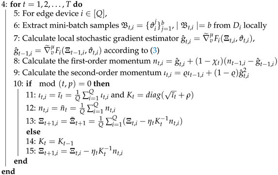
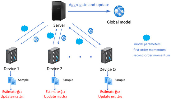
Figure 1. FAFedZO framework.

4. Convergence Analysis of FAFedZO Method

In this section, the convergence of the FAFedZO method will be discussed. To facilitate the theoretical analysis of the proposed algorithm, we need to make some assumptions as follows.

Assumption 1. 

The global loss function $f(\mathbf{\Xi })$ in (1) has a lower bound, that is, there is a fixed value $f^{*}$ that exists $f(\mathbf{\Xi })\ge f^{*}>-\infty .$

Assumption 1 means that regardless of the value of the optimization variable $\mathbf{\Xi }$, the global loss function $f(\mathbf{\Xi })$ will not decrease indefinitely, and there exists a minimum value $f^{*}$, ensuring that the optimal solution we are looking for is within a meaningful range. Otherwise, the algorithm may keep trying to find a lower value and fail to converge.

Assumption 2. 

We suppose that functions $F_i(\mathbf{\Xi },{\vartheta }_i),f_i(\mathbf{\Xi }),f(\mathbf{\Xi })$ are all L-smooth; that is, for all ${\mathbf{\Xi }}_1\in R^d,{\mathbf{\Xi }}_2\in R^d$, we can conclude that

$$\begin{array}{c}\hfill \parallel \nabla f_i\left({\mathbf{\Xi }}_1\right)-\nabla f_i\left({\mathbf{\Xi }}_2\right)\parallel \le L\parallel {\mathbf{\Xi }}_1-{\mathbf{\Xi }}_2\parallel ,\end{array}$$

where $L>0$ represents the Lipschitz constant, and $\parallel ·\parallel$ represents the $l_2$ norm. In addition, it can also be expressed in the form of $f\left({\mathbf{\Xi }}_1\right)\le f\left({\mathbf{\Xi }}_2\right)+⟨\nabla f\left({\mathbf{\Xi }}_2\right),{\mathbf{\Xi }}_1-{\mathbf{\Xi }}_2⟩+{\displaystyle \frac{L}{2}}{\parallel {\mathbf{\Xi }}_1-{\mathbf{\Xi }}_2\parallel }^2$, where the symbol $⟨·,·⟩$ represents the inner product.

Assumption 2 is common in the theoretical analysis of non-convex optimization [24,27], indicating that the gradient changes of $f_i(\mathbf{\Xi })$, $f(\mathbf{\Xi })$ are smooth and do not change suddenly. It is widely used in optimization analysis, and many typical federated learning algorithms have adopted this assumption, such as Fed-GLOMO [22], STEM [23], and so on.

Assumption 3. 

$\nabla F_i(\mathbf{\Xi },{\vartheta }_i)$ serves as a precise approximation of $\nabla f_i(\mathbf{\Xi })$ without bias, namely

$$E_{{\vartheta }_i}[\nabla F_i(\mathbf{\Xi },{\vartheta }_i)]=\nabla f_i(\mathbf{\Xi }),\forall \mathbf{\Xi }\in R^d.$$

Assumption 3 is usually used in stochastic optimization. It allows us to approximate the true gradient by using the gradient of random sampling, thus reducing the computational complexity. This is because, especially in the cases of large-scale data and complex models, it is often infeasible to calculate the gradient precisely.

Assumption 4. 

The variance of the stochastic gradient is limited within a certain range; that is, there is a constant ${\sigma }_g>0$ that satisfies

$$E_{{\vartheta }_i}{\parallel \nabla F_i(\mathbf{\Xi },{\vartheta }_i)-\nabla f_i(\mathbf{\Xi })\parallel }^2\le {\sigma }_g^2,\forall \mathbf{\Xi }\in R^d.$$

Assumption 4 indicates that the variance of stochastic gradients will not be infinite. If the variance is too large, the algorithm may experience violent oscillations during the optimization process and fail to converge. Bounded variance is a necessary condition for controlling the noise of SGD and ensuring the convergence rate.

Assumption 5. 

The difference between each local loss function and the global loss function remains within a certain limit; that is, there exists a constant ${\sigma }_h>0$ that satisfies

$$\parallel \nabla f(\mathbf{\Xi })-\nabla f_i{(\mathbf{\Xi })\parallel }^2\le {\sigma }_h^2,\forall \mathbf{\Xi }\in R^d.$$

Assumption 5 is used to describe the heterogeneity between the local loss and the global loss and is also taken into account in distributed zero-order optimization [37]. It ensures that local optimization will not lead to a significant decline in global performance.

Assumption 6. 

The inter-node variance is bounded, namely,

$$\parallel \nabla f_i(\mathbf{\Xi })-\nabla f_j{(\mathbf{\Xi })\parallel }^2\le {\zeta }^2,\forall \mathbf{\Xi }\in R^d,$$

where ζ is the heterogeneity parameter, which represents the level of data heterogeneity.

Assumption 6 is a typical assumption used to constrain data heterogeneity in the federated learning algorithm. When the data are set to be IID, that is, for all $i,j\in \left[Q\right]$, $D_i=D_j$, then $\zeta =0$. This assumption indicates that the differences between the loss functions on different devices are limited, ensuring that the optimization processes on different devices will not deviate too much.

Assumption 7. 

In our algorithms, for all $t\ge 1$, the adaptive matrx $K_t$ satisfies the condition that

$${\lambda }_{min}\left(K_t\right)\ge \rho >0,$$

where ρ represents an appropriate positive value and ${\lambda }_{min}(·)$ represents the minimum eigenvalue of a matrix.

Assumption 7 ensures that the adaptive matrix $K_t$ is positive definite for any $t\ge 1$. By ensuring that the minimum eigenvalue is greater than the positive number $\rho$, it can guarantee that the algorithm has a sufficient update step size in each iteration, thus ensuring the convergence of the algorithm.

Assumption 8. 

The gradients of function $f_i(\mathbf{\Xi })$ are G-bounded; that is, for all i, $\mathbf{\Xi }\in R^d$, we have

$$\parallel \nabla f_i(\mathbf{\Xi })\parallel \le G.$$

where $G>0$ is a positive constant.

Assumption 8 provides an upper bound for the gradient in the adaptive method. This is a typical assumption in the adaptive method, which is used to constrain the upper bound of the adaptive learning rate. This is reasonable and can usually be satisfied in practice. For example, it holds for the finite sum problem.

In the context of optimization algorithms, in order to prove the final specific conclusion, we need to introduce the concept of the $ϵ$-stationary point. We define the $ϵ$-stationary point as follows:

Definition 1. 

A point Ξ is called ϵ-stationary if $\parallel \nabla f(\mathbf{\Xi })\parallel \le ϵ$. Generally, a stochastic algorithm is defined to achieve an ϵ-stationary point in T iterations if $\mathbb{E}\parallel \nabla f\left({\mathbf{\Xi }}_T\right)\parallel \le ϵ$.

Then, we investigate the convergence characteristics of our novel method based on Assumptions 1–8. We first obtain the following six lemmas:

Lemma 1 gives the upper bound of the adaptive matrix $K_t$.

Lemma 1. 

Suppose the adaptive matrix sequence ${\left\{K_t\right\}}_{t=1}^T$ is derived from the algorithm. On the basis of Assumptions 1–8, we can conclude that

$$\begin{array}{c}\hfill \mathbb{E}{∥K_t∥}^2\le 2d(G^2+{\sigma }_g^2)+2{\rho }^2+{\displaystyle \frac{1}{2}}{d}^2{L}^2{\mu }^2\end{array}$$

(6)

Lemma 2 measures the boundary of variance between gradients.

Lemma 2. 

For $i\in \left[Q\right]$, where $\left[Q\right]$ represents all Q edge devices from 1 to Q, we can conclude that

$$\begin{array}{cc}\hfill & \mathbb{E}\parallel {\tilde{\nabla }}_v^{\mu }{F}_i({\mathbf{\Xi }}_{t,i};{\mathfrak{B}}_{t,i})-g_{t,i}{\parallel }^2\le L^2{\mu }^2\hfill \end{array}$$

(7)

$$\begin{array}{cc}\hfill & \mathbb{E}\parallel g_t-\mathbf{1}\otimes {\overline{g}}_t{\parallel }^2\le 6L^2\mathbb{E}{\parallel {\mathbf{\Xi }}_t-\mathbf{1}\otimes {\overline{\mathbf{\Xi }}}_t\parallel }^2+3Q{\zeta }^2\hfill \end{array}$$

(8)

Lemma 3 studies the bounds under different values of ${\sum }_{i=1}^Q{∥{\mathbf{\Xi }}_{t,i}-{\overline{\mathbf{\Xi }}}_t∥}^2$, which is important for the proof of the subsequent theorems.

Lemma 3. 

Given that $t\in [\lfloor t/p\rfloor p,\lfloor t/p\rfloor (p+1\left)\right]$, ${\mathbf{\Xi }}_t$ is derived from the algorithm; we can conclude that

(1) If $t=s_t=\lfloor t/p\rfloor p$, then we can obtain

$$\begin{array}{c}\hfill \sum _{i=1}^Q{∥{\mathbf{\Xi }}_{s_t,i}-{\overline{\mathbf{\Xi }}}_{s_t}∥}^2=0\end{array}$$

(9)

(2) If $t\ge \lfloor t/p\rfloor p$, then we can obtain

$$\begin{array}{c}\hfill \sum _{i=1}^Q{∥{\mathbf{\Xi }}_{t,i}-{\overline{\mathbf{\Xi }}}_t∥}^2\le (p-1)\sum _{s=s_t}^{t-1}{\eta }_s^2\sum _{i=1}^Q{\parallel K_s^{-1}(n_{s,i}-{\overline{n}}_s)\parallel }^2\end{array}$$

(10)

Lemma 4 gives the relationship between the expected values of the function f at the model parameters ${\overline{\mathbf{\Xi }}}_{t+1}$ and ${\overline{\mathbf{\Xi }}}_t$.

Lemma 4. 

Assuming the sequence ${\left\{{\mathbf{\Xi }}_t\right\}}_0^T$ is generated by the algorithm, then we can obtain

$$\begin{array}{cc}\hfill \mathbb{E}f\left({\overline{\mathbf{\Xi }}}_{t+1}\right)& \le \mathbb{E}f\left({\overline{\mathbf{\Xi }}}_t\right)-({\displaystyle \frac{3\rho }{4{\eta }_t}}-{\displaystyle \frac{L}{2}})\mathbb{E}\parallel {\overline{\mathbf{\Xi }}}_{t+1}-{\overline{\mathbf{\Xi }}}_t{\parallel }^2-{\displaystyle \frac{{\eta }_t}{4\rho }}\mathbb{E}\parallel \nabla f\left({\overline{\mathbf{\Xi }}}_t\right)-{\overline{n}}_t{\parallel }^2+{\displaystyle \frac{5{\eta }_t}{2\rho }}\mathbb{E}{\parallel {\overline{g}}_t-{\overline{n}}_t\parallel }^2\hfill \\ \hfill & +{\displaystyle \frac{5{\eta }_t{L}^2}{2\rho Q}}\mathbb{E}{\parallel {\mathbf{\Xi }}_t-\mathbf{1}\otimes {\overline{\mathbf{\Xi }}}_t\parallel }^2\hfill \end{array}$$

(11)

Lemma 5 gives the iterative relationship between $\mathbb{E}\parallel {\overline{n}}_t-{\overline{g}}_t{\parallel }^2$ and $\mathbb{E}\parallel {\overline{n}}_{t-1}-{\overline{g}}_{t-1}{\parallel }^2$.

Lemma 5. 

Suppose that $n_t$ they are produced by the algorithm; we subsequently obtain

$$\begin{array}{c}\hfill \mathbb{E}\parallel {\overline{n}}_t-{\overline{g}}_t{\parallel }^2\le 2{(1-{\chi }_t)}^2\mathbb{E}\parallel {\overline{n}}_{t-1}-{\overline{g}}_{t-1}{\parallel }^2+{\displaystyle \frac{4{(1-{\chi }_t)}^2{L}^2}{Q}}\mathbb{E}{\parallel {\mathbf{\Xi }}_t-{\mathbf{\Xi }}_{t-1}\parallel }^2+4{\chi }_t^2{L}^2{\mu }^2\end{array}$$

(12)

Lemma 6 is also a crucial conclusion for proving the final theorem.

Lemma 6. 

Suppose that $n_t$ is produced by the algorithm; we subsequently obtain

$$\begin{array}{c}\hfill {\displaystyle \frac{30\rho }{72Q}}\sum _{t=s_t}^{\overline{s}}{\eta }_t\sum _{i=1}^Q\mathbb{E}\parallel K_t^{-1}(n_{t,i}-{\overline{n}}_t){\parallel }^2\le {\displaystyle \frac{\rho }{4}}\sum _{t=s_t}^{\overline{s}}{\displaystyle \frac{1}{{\eta }_t}}\mathbb{E}{\parallel {\overline{\mathbf{\Xi }}}_{t+1}-{\overline{\mathbf{\Xi }}}_t\parallel }^2+\left[{\displaystyle \frac{\rho {\mu }^2{c}^2}{4Q}}+{\displaystyle \frac{3\rho {\zeta }^2{c}^2}{4L^2}}\right]\sum _{t=s_t}^{\overline{s}}{\eta }_t^3\end{array}$$

(13)

The proofs of these lemmas are provided in Appendix A. Then, based on the conclusions of the above lemmas, we can prove the final convergence theorem:

Theorem 1. 

Assume that the sequence ${\left\{{\overline{\mathbf{\Xi }}}_t\right\}}_{t=1}^T$ is produced by Algorithm 1. Based on Assumptions 1–8, given that $\forall t\ge 0$, ${\chi }_{t+1}=c·{\eta }_t^2$, $c={\displaystyle \frac{1}{12Lp{\overline{h}}^3{\rho }^2}}+{\displaystyle \frac{30L^2}{{\rho }^2}}\le {\displaystyle \frac{60L^2}{{\rho }^2}}$, $w_t=max({\displaystyle \frac{3}{2}},1728L^3{p}^3{\overline{h}}^3-t)$, $\overline{h}={\displaystyle \frac{1}{L}}$ and

$$\begin{array}{c}\hfill {\eta }_t={\displaystyle \frac{\rho \overline{h}}{{\left(w_t+t\right)}^{1/3}}}\end{array}$$

(14)

we can conclude that

$$\begin{array}{cc}\hfill {\displaystyle \frac{1}{T}}\sum _{t=1}^T\mathbb{E}\parallel \nabla f\left({\overline{\mathbf{\Xi }}}_t\right)\parallel & \le P[\left[{\displaystyle \frac{12Lp}{{\rho }^{2}T}}+{\displaystyle \frac{L}{{\rho }^2{T}^{2/3}}}\right]\mathbb{E}\left[f\left({\overline{\mathbf{\Xi }}}_0\right)-f^{*}\right]+{\displaystyle \frac{6L^2{\mu }^2{p}^2}{{\rho }^{2}QT}}\hfill \\ \hfill & +\left[{\displaystyle \frac{{12}^2\times 75p}{{\rho }^{2}T}}+{\displaystyle \frac{900}{{\rho }^2{T}^{2/3}}}\right]\left[{\displaystyle \frac{5L^2{\mu }^2}{3}}+3{\zeta }^2\right](lnT+1)\hfill \\ \hfill & +{\displaystyle \frac{L^2{\mu }^{2}p}{2{\rho }^{2}Q{T}^{2/3}}}{]}^{1/2},\hfill \end{array}$$

(15)

where $P=5\sqrt{2d(G^2+{\sigma }_g^2)+2{\rho }^2+{\displaystyle \frac{1}{2}}{d}^2{L}^2{\mu }^2}$.

Due to limited space, we will only briefly introduce the outline of the proof here: Firstly, by combining the objective function $f\left({\overline{\mathbf{\Xi }}}_t\right)$ and the gradient estimation error term, we construct a Lyapunov function ${\Gamma }_t$ for analysis. Secondly, we establish a recurrence inequality for ${\Gamma }_t$. Through cumulative summation, we can estimate the bounds and convergence of the term ${\displaystyle \frac{1}{T}}{\sum }_{t=0}^{T-1}\mathbb{E}\left[{\displaystyle \frac{1}{12{\eta }_t^2}}{∥{\overline{\mathbf{\Xi }}}_{t+1}-{\overline{\mathbf{\Xi }}}_t∥}^2+{\displaystyle \frac{1}{4{\rho }^2}}{∥\nabla f\left({\overline{\mathbf{\Xi }}}_t\right)-{\overline{n}}_t∥}^2\right]$. Finally, based on the above, we can derive the convergence bound of the objective function ${\displaystyle \frac{1}{T}}{\sum }_{t=1}^T\mathbb{E}\parallel \nabla f\left({\overline{\mathbf{\Xi }}}_t\right)\parallel$.

The detailed proof of Theorem 1 can be found in Appendix A.

Remark 1. 

We utilize ζ as an indicator of data heterogeneity. The final results demonstrate that an increase in ζ (indicating greater data heterogeneity) leads to a slowdown in the training process. In addition, we consider that the step size ${\mu }_t$ remains unchanged during the training process. Therefore, we omit its subscript and represent it with μ.

Remark 2. 

A suitable value of ρ ensures a balanced incorporation of adaptive information in the learning rate. In practice, we commonly select ρ to be within the order of $O\left(1\right)$, steering clear of excessively small or large values.

Remark 3 

(Computational complexity). For ${\mathcal{Q}}_t={\displaystyle \frac{1}{12{\eta }_t^2}}{∥{\overline{\mathbf{\Xi }}}_{t+1}-{\overline{\mathbf{\Xi }}}_t∥}^2+{\displaystyle \frac{1}{4{\rho }^2}}{∥\nabla f\left({\overline{\mathbf{\Xi }}}_t\right)-{\overline{n}}_t∥}^2$, we have

$$\begin{array}{cc}\hfill {\displaystyle \frac{1}{T}}\sum _{t=0}^{T-1}\mathbb{E}\left[{\mathcal{Q}}_t\right]& ={\displaystyle \frac{1}{T}}\sum _{t=0}^{T-1}\mathbb{E}\left[{\displaystyle \frac{1}{12{\eta }_t^2}}{∥{\overline{\mathbf{\Xi }}}_{t+1}-{\overline{\mathbf{\Xi }}}_t∥}^2+{\displaystyle \frac{1}{4{\rho }^2}}{∥\nabla f\left({\overline{\mathbf{\Xi }}}_t\right)-{\overline{n}}_t∥}^2\right]\hfill \\ \hfill & \le \left[{\displaystyle \frac{12Lp}{{\rho }^{2}T}}+{\displaystyle \frac{L}{{\rho }^2{T}^{2/3}}}\right]\mathbb{E}\left[f\left({\overline{\mathbf{\Xi }}}_0\right)-f^{*}\right]+{\displaystyle \frac{6L^2{\mu }^2{p}^2}{{\rho }^{2}QT}}+{\displaystyle \frac{L^2{\mu }^{2}p}{2{\rho }^{2}Q{T}^{2/3}}}\hfill \\ \hfill & +\left[{\displaystyle \frac{{12}^2\times 75p}{{\rho }^{2}T}}+{\displaystyle \frac{900}{{\rho }^2{T}^{2/3}}}\right]\left[{\displaystyle \frac{5L^2{\mu }^2}{3}}+3{\zeta }^2\right](lnT+1)\hfill \end{array}$$

Referring to the method in [38], without loss of generality, we let ${\displaystyle \frac{p}{Q}}=O\left(1\right)$ and choose $p=T^{{\displaystyle \frac{1}{3}}}$. To make the right side of the inequality less than ${ϵ}^2$, we can obtain $T=O\left({ϵ}^{-3}\right)$ and ${\displaystyle \frac{T}{p}}=T^{{\displaystyle \frac{2}{3}}}={ϵ}^{-2}$. Therefore, to satisfy the definition of an ϵ-stationary point, which is $\mathbb{E}\parallel \nabla f\left({\mathbf{\Xi }}_T\right)\parallel \le ϵ$ and $\mathbb{E}\left[{\mathcal{Q}}_t\right]\le {ϵ}^2$, we obtain the total sample cost as $O\left({ϵ}^{-3}\right)$ and the communication round as $O\left({ϵ}^{-2}\right)$.

Remark 4 

(Convergence speed). In the FedZO algorithm [27], regardless of whether all devices participate or only partial devices participate, we can observe that the FedZO algorithm achieves a convergence rate of $O\left({\displaystyle \frac{1}{T^{1/2}}}\right)$. Furthermore, as indicated by Theorem 1, our algorithm can achieve a convergence rate of $O\left({\displaystyle \frac{1}{T^{2/3}}}\right)$. Therefore, our FAFedZO method theoretically possesses a faster convergence rate compared to general zero-order methods. This further validates the advantages of our approach.

5. Experimental Results

In this section, we conduct comparative experiments on the MNIST, CIFAR-10 and Fashion-MNIST datasets and present some experimental outcomes to assess the performance of the proposed FAFedZO method in federated black-box attacks, thereby confirming the advantages of this algorithm.

5.1. Experimental Environment and Datasets

Experimental environment configuration: This study utilizes the FedZO framework as the experimental baseline to conduct research on federated learning algorithms. For this study, Python version 3.10.13 is adopted as the programming language, and PyTorch 2.2.0 serves as the development platform. All tests are conducted on a Windows 10 platform equipped with an NV GTX1650 GPU version 572.83 and CUDA version 12.4.99.

Dataset: We conduct comparative experimental studies on the MNIST, CIFAR-10 and Fashion-MNIST datasets.

The MNIST dataset is a classic handwritten digit image dataset. This dataset comprises a collection of grayscale images of handwritten digits (0–9) with 60,000 training samples and 10,000 test samples, with each image measuring 28 × 28 pixels. The CIFAR-10 dataset consists of 60,000 32 × 32 color images across 10 categories, each category contains 6000 images, and the dataset is divided into 50,000 training and 10,000 test images. The Fashion-MNIST dataset has the same data structure as the MNIST dataset, containing 10 categories of grayscale images representing different types of clothing like T-shirts, trousers, sweaters, and so on.

5.2. Experimental Result Analysis

Here, we present the results of simulation experiments to assess the performance of the FAFedZO method in the context of black-box attack strategies.

Given the characteristics of black-box scenarios, optimizing black-box attacks falls into the realm of zero-order optimization. We investigate black-box attacks on a trained deep neural network (DNN) classification model. An attack refers to an intentional attempt to manipulate the input data of a model so as to interfere with its normal operation. It can be achieved by adding carefully designed perturbations to the original data, for example, the interference images that we aim to train on in this experiment. The normal learning process is based on the assumption that the input data follow a certain distribution. However, when under attack, the introduced adversarial examples will violate this distribution assumption. This will force the model to make incorrect predictions, and if this kind of attack is not properly dealt with, it may lead to the failure of the model’s generalization ability. The purpose of our experiment is to train an interference image with the same size as the image in the dataset, which makes it difficult for the human eyes to recognize the difference between the original image and the adversarial image after adding the interference image, but it can induce the classification model to make a wrong judgment. We want to achieve a higher attack success rate with as little disturbance as possible, so we consider the loss function shown below:

$$\begin{array}{cc}\hfill & \psi (\mathbf{\Xi },\vartheta )\hfill \\ \hfill =& \underset{I}{\underbrace{max\left\{{\phi }_{y_{\vartheta }}\left({\displaystyle \frac{1}{2}}tanh\left(tan{h}^{-1}2\vartheta +\mathbf{\Xi }\right)\right)-{max}_{j\ne y_{\vartheta }}\left\{{\phi }_j\left({\displaystyle \frac{1}{2}}tanh\left(tan{h}^{-1}2\vartheta +\mathbf{\Xi }\right)\right)\right\},0\right\}}}\hfill \\ \hfill +& c\underset{II}{\underbrace{{∥{\displaystyle \frac{1}{2}}tanh\left(tan{h}^{-1}2\vartheta +\mathbf{\Xi }\right)-\vartheta ∥}^2}}\hfill \end{array}$$

(16)

where $\mathbf{\Xi }$ represents the interference image to be trained, $\vartheta$ represents the original image in the dataset, $y_{\vartheta }$ represents the label corresponding to the image $\vartheta$ (for example, the label of the image “deer” is 4), and ${\phi }_j\left(\vartheta \right)$ represents the confidence that the classification model recognizes image $\vartheta$ as label j. The item I in Equation (16) measures the probability of attack failure (marked as attack loss), $II$ represents the image distortion caused by disturbance, and c is the balance coefficient. In this way, our goal can be achieved by minimizing $\psi (\mathbf{\Xi },\vartheta )$. Next, we use Equation (16) to construct the local loss function.

We divide the samples in the dataset into Q groups randomly and unevenly without repetition and then distribute them to each edge device, where Q is the total count of edge devices we preset. Then, for all edge devices, we define their local loss function as

$$\begin{array}{c}\hfill f_i(\mathbf{\Xi })\triangleq E_{{\vartheta }_i\sim D_i}\left[\psi (\mathbf{\Xi },{\vartheta }_i)\right],i\in \{1,2,\dots ,Q\}\end{array}$$

(17)

where $D_i$ represents the dataset at the ith edge device. In this way, the federal black-box attack problem on the DNN classification model can be formulated as a federated optimization problem: $f(\mathbf{\Xi })\triangleq {\displaystyle \frac{1}{Q}}{\sum }_{i=1}^Q{f}_i(\mathbf{\Xi })$. Next, we use the FAFedZO algorithm proposed in this paper to solve this problem.

We select balance parameter $c=1$. For the remaining parameters, we select them as $(b_1,b_2,\mu )=(25,20,0.001)$ and set the initial learning rate $\eta$ to be 0.1.

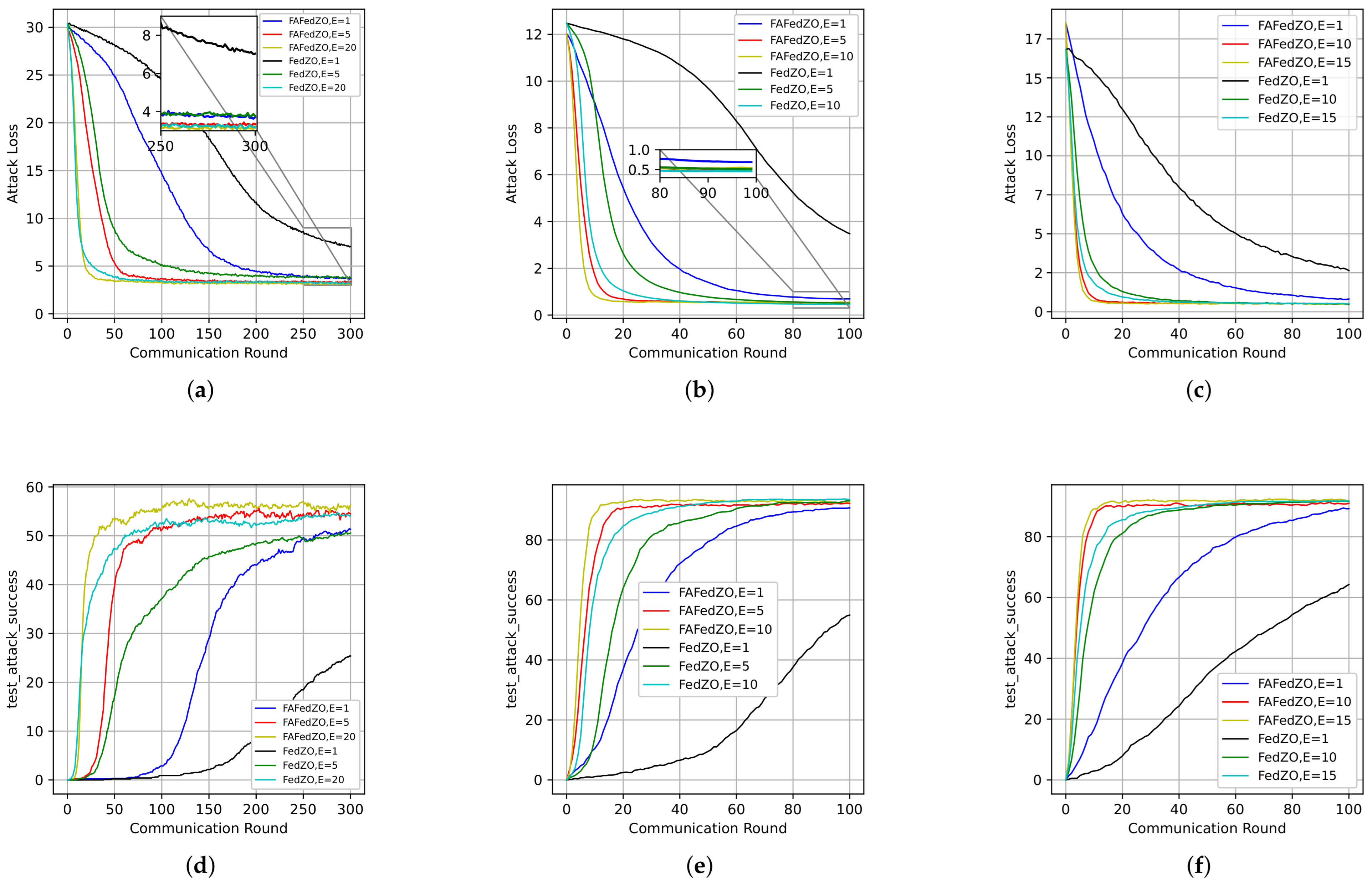
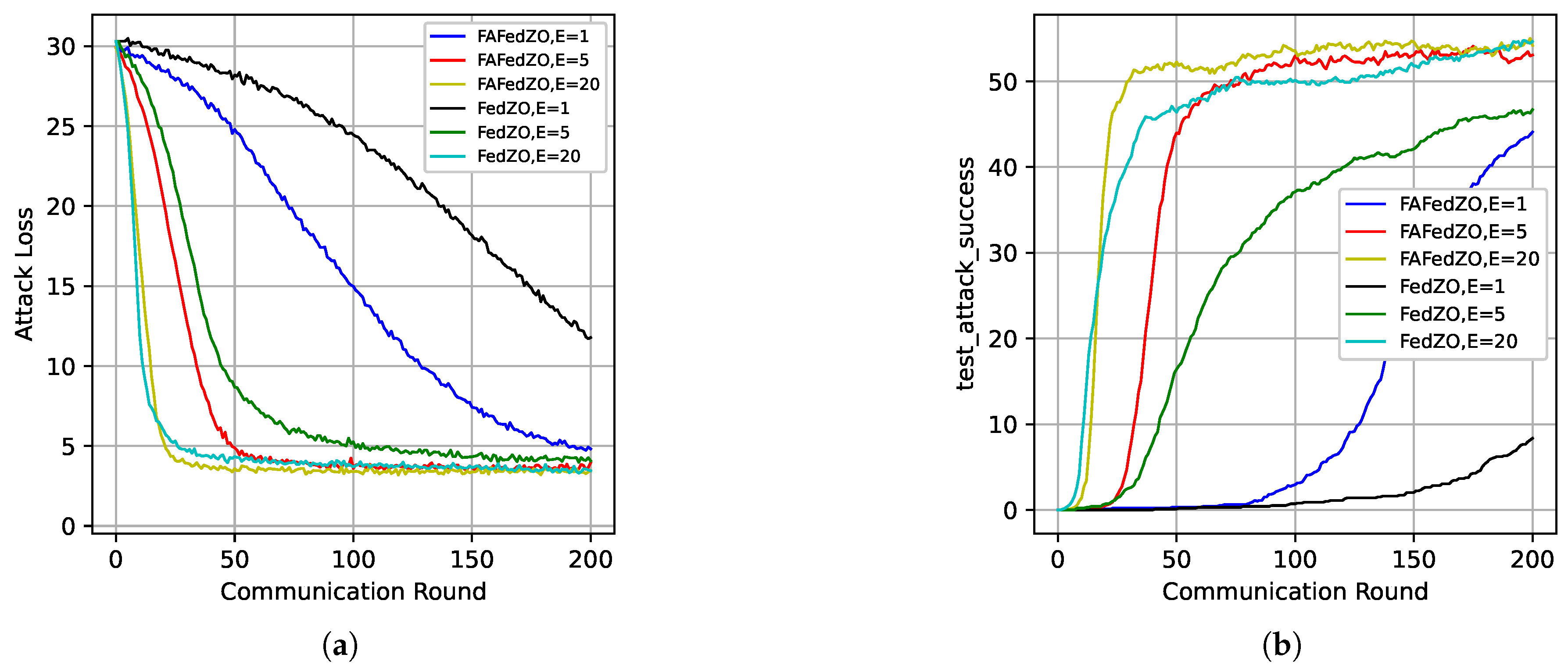
We select the total number of edge devices $Q=50$ and the number of participating edge devices $M=30$ and study the influence of the number of local updates E on the attack loss and attack accuracy of the proposed FAFedZO algorithm. Then, we compare it with the FedZO algorithm. We conduct experiments on the MNIST, CIFAR-10, and Fashion-MNIST datasets, respectively, and the results are shown in Figure 2.

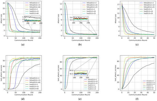
Figure 2. Influence of varying the number of local updates that select $(Q,M)=(50,30)$. (a) The attack loss on the MNIST dataset. (b) The attack loss on the CIFAR-10 dataset. (c) The attack loss on the Fashion-MNIST dataset. (d) The testing accuracy on the MNIST dataset. (e) The testing accuracy on the CIFAR-10 dataset. (f) The testing accuracy on the Fashion-MNIST dataset.

Taking the MNIST dataset as an example, Figure 2a,d illustrate the impact of the number of local updates $E\in \{3,15,60\}$ on the performance of the algorithm. It can be observed that the larger the value of E, the lower the attack loss of the algorithm and the higher the accuracy. In addition, the attack accuracy of FAFedZO is significantly higher than that of FedZO. When $E=60$, they achieve comparable accuracy, which proves that the algorithm proposed in this paper is superior to the original FedZO algorithm. Similar results can also be obtained on the remaining two datasets.

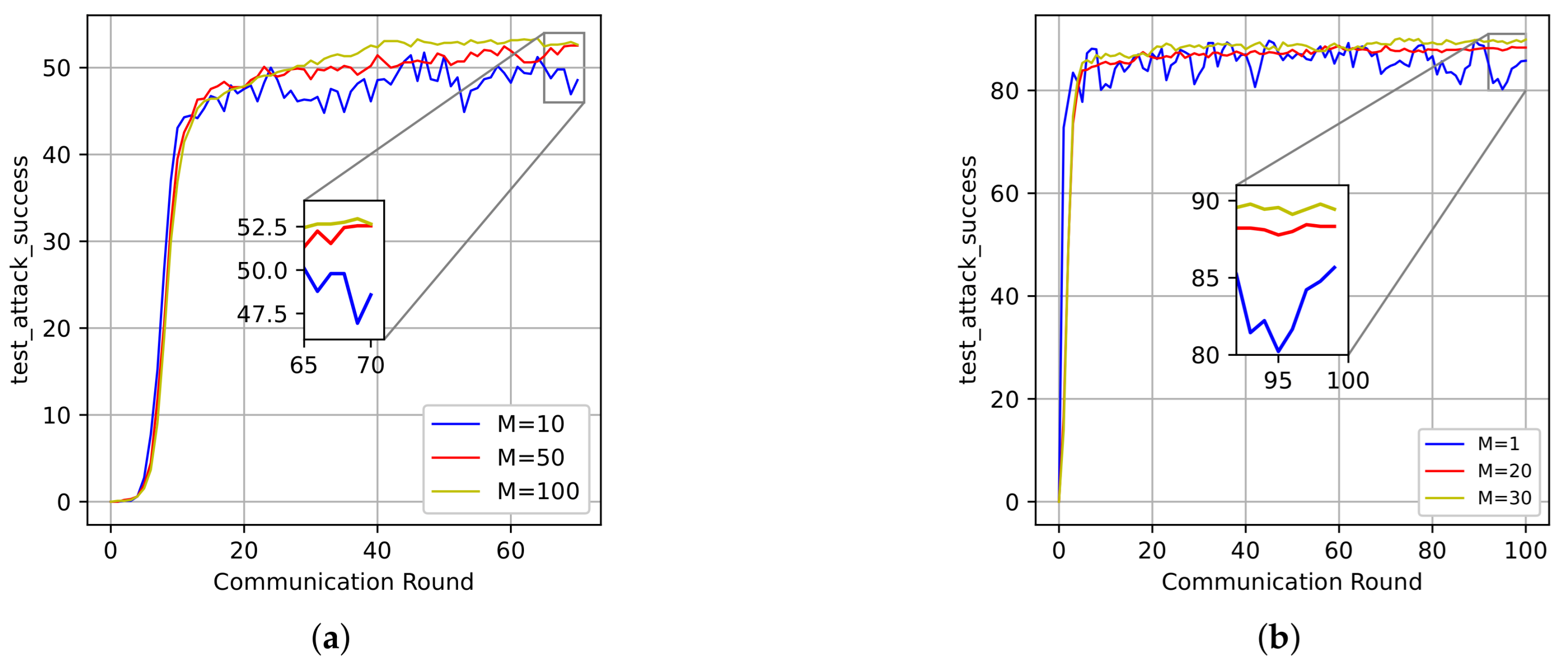
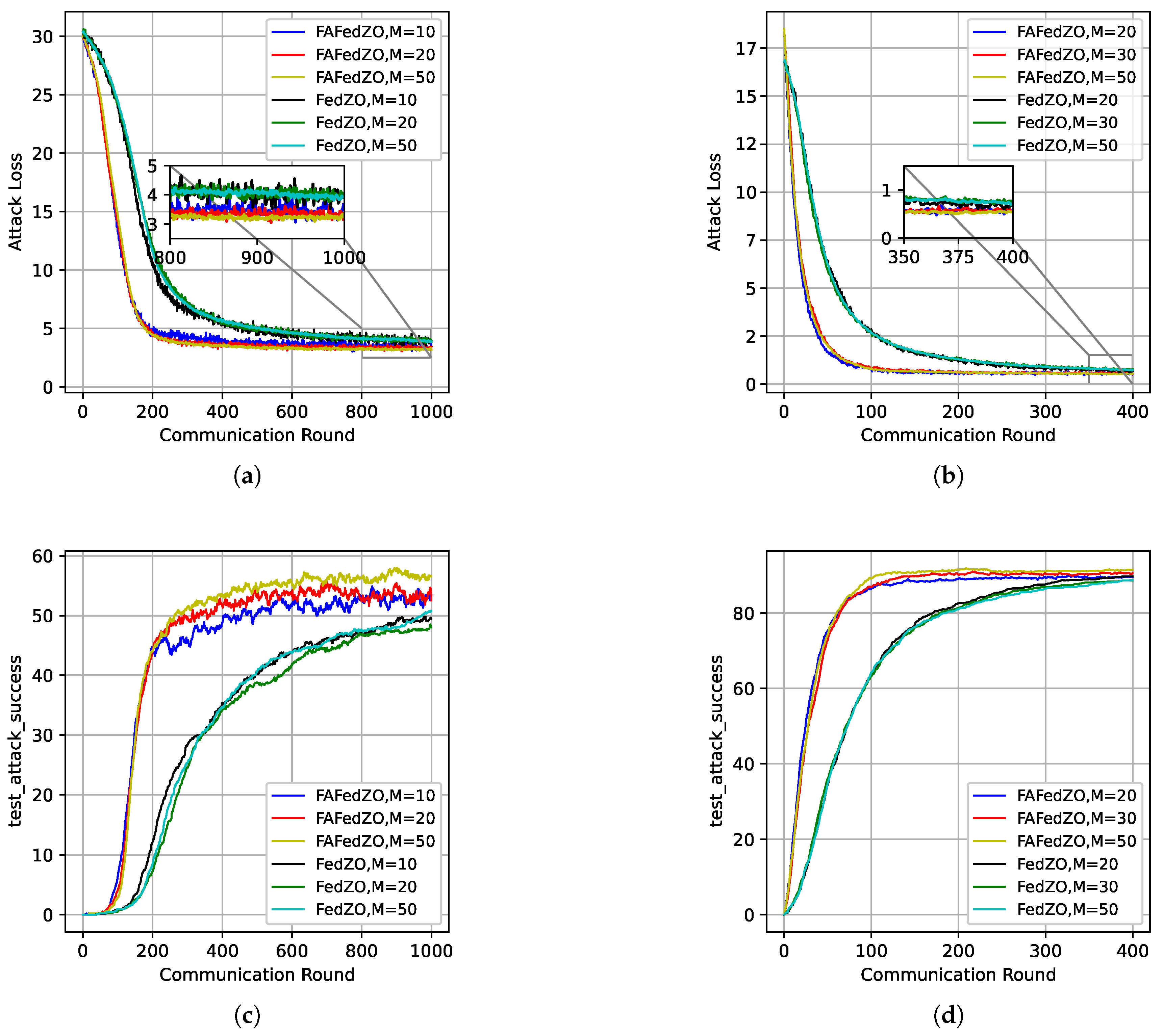
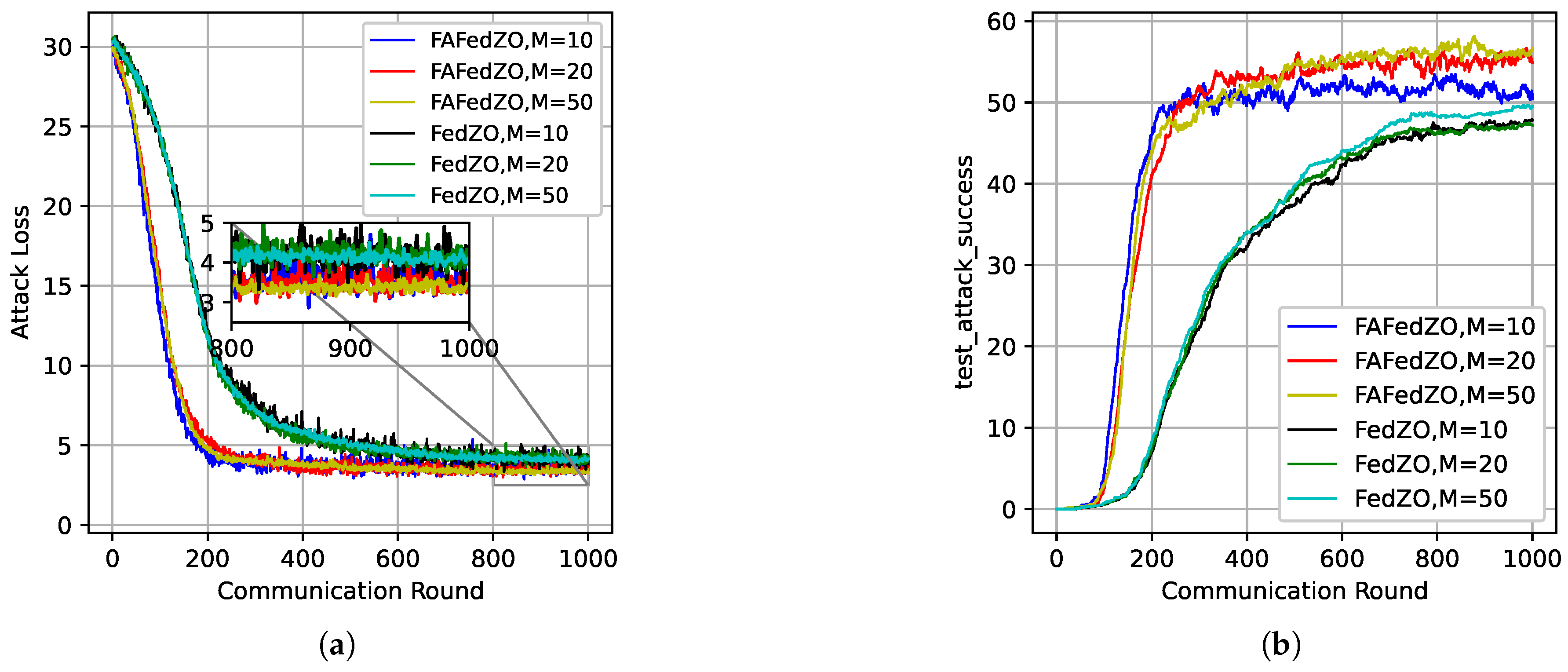
In Figure 3, with the total number of edge devices $Q=100$ and the number of local updates $E=60$, the impact of the number M of participating edge devices on the convergence performance of the FAFedZO method is studied on the MNIST and Fashion-MNIST datasets. It can be seen that by adjusting the value of M, the FAFedZO algorithm can effectively enhance the attack accuracy.

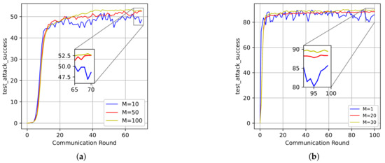
Figure 3. Influence of the number of participating edge devices that select $(Q,E)=(100,60)$. (a) The testing accuracy on the MNIST dataset. (b) The testing accuracy on the Fashion-MNIST dataset.

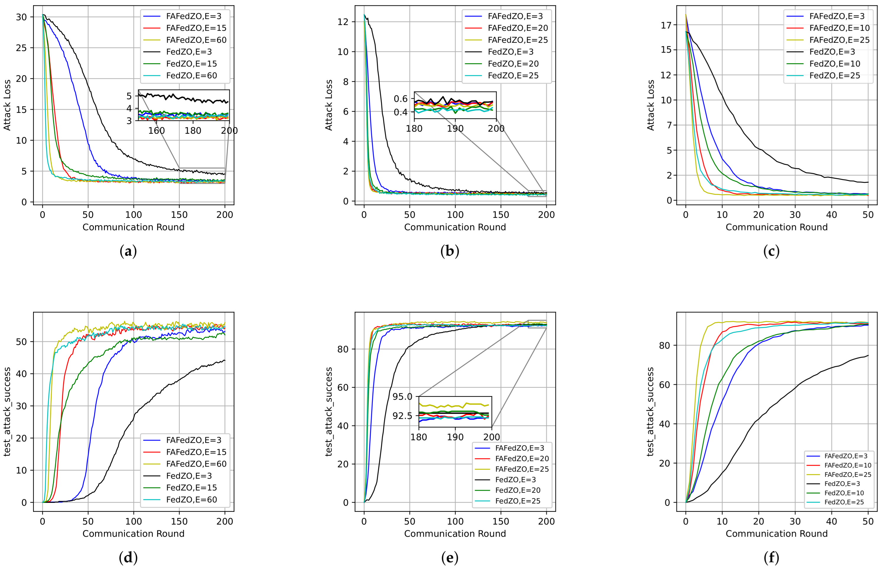
In Figure 4, we select the parameters $Q=50$ and $M=50$; that is, when all devices are involved, to study the impact of the number of local updates E on the convergence performance of the algorithm. We have also conducted experiments on the MNIST, CIFAR-10, and Fashion-MNIST datasets, respectively. It is obvious that, compared with the FedZO algorithm under different values of E, the FAFedZO method can significantly reduce the attack loss and improve the attack accuracy. Moreover, as the value of E increases, the convergence speed of the FAFedZO algorithm also accelerates, with lower attack loss and higher attack accuracy, and both tend to stabilize more quickly.

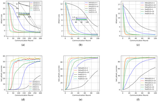
Figure 4. Influence of the number of local updates that select $Q=50$ and $M=50$. (a) The attack loss on the MNIST dataset. (b) The attack loss on the CIFAR-10 dataset. (c) The attack loss on the Fashion-MNIST dataset. (d) The testing accuracy on the MNIST dataset. (e) The testing accuracy on the CIFAR-10 dataset. (f) The testing accuracy on the Fashion-MNIST dataset.

Finally, we study the impact of the number of participating edge devices M on the algorithm under the conditions of $Q=50$ and $E=1$. We conducted experiments on the MNIST and Fashion-MNIST datasets, and the results are shown in Figure 5. It can be seen that the FAFedZO algorithm far outperforms the FedZO algorithm in terms of both attack loss and accuracy. Even when the FedZO algorithm takes the optimal value among the selected values of M, its performance is still weaker than the worst value of the FAFedZO algorithm. In addition, as M increases, the attack loss value decreases and the accuracy increases, which is in line with our expectations.

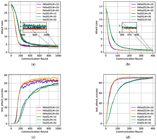
Figure 5. Influence of the number of participating edge devices that select $Q=50$ and $E=1$. (a) The attack loss on the MNIST dataset; (b) The attack loss on the Fashion-MNIST dataset; (c) The testing accuracy on the MNIST dataset; (d) The testing accuracy on the Fashion-MNIST dataset.

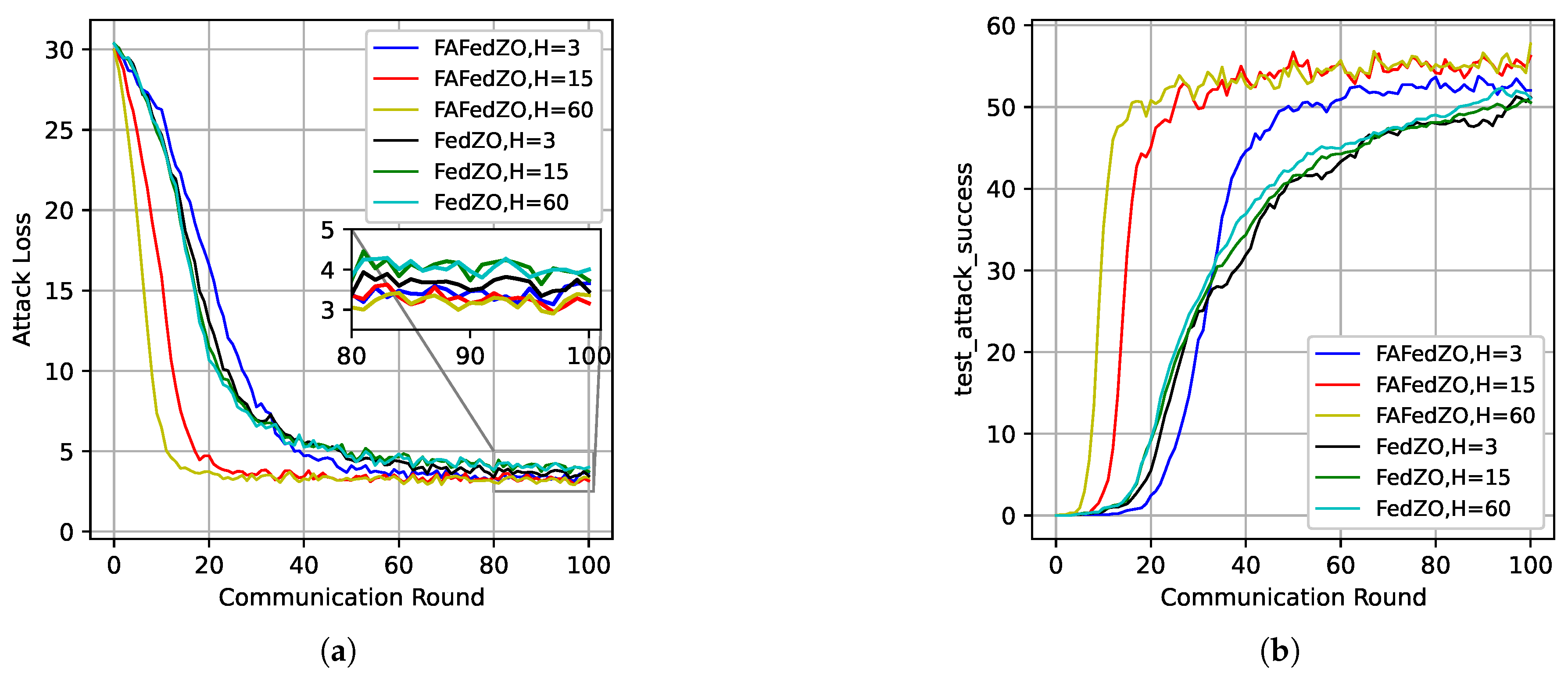
In addition to investigating the impact of the number of local updates and the number of participating edge devices on the algorithm’s performance, we also study the influence of varying the number of random directions on the proposed algorithm. As shown in Figure 6, on the MNIST dataset, under the conditions of $Q=50$ and $M=10$, we present the curves illustrating the impact of the number of directions $H\in \{3,15,60\}$ on attack loss and attack accuracy. It can be observed that we have similar conclusions to the above figures, which further confirms the superiority of the FAFedZO algorithm.

Figure 6. Influence of the number of directions that select $Q=50$ and $M=10$. (a) Attack loss; (b) Testing accuracy.

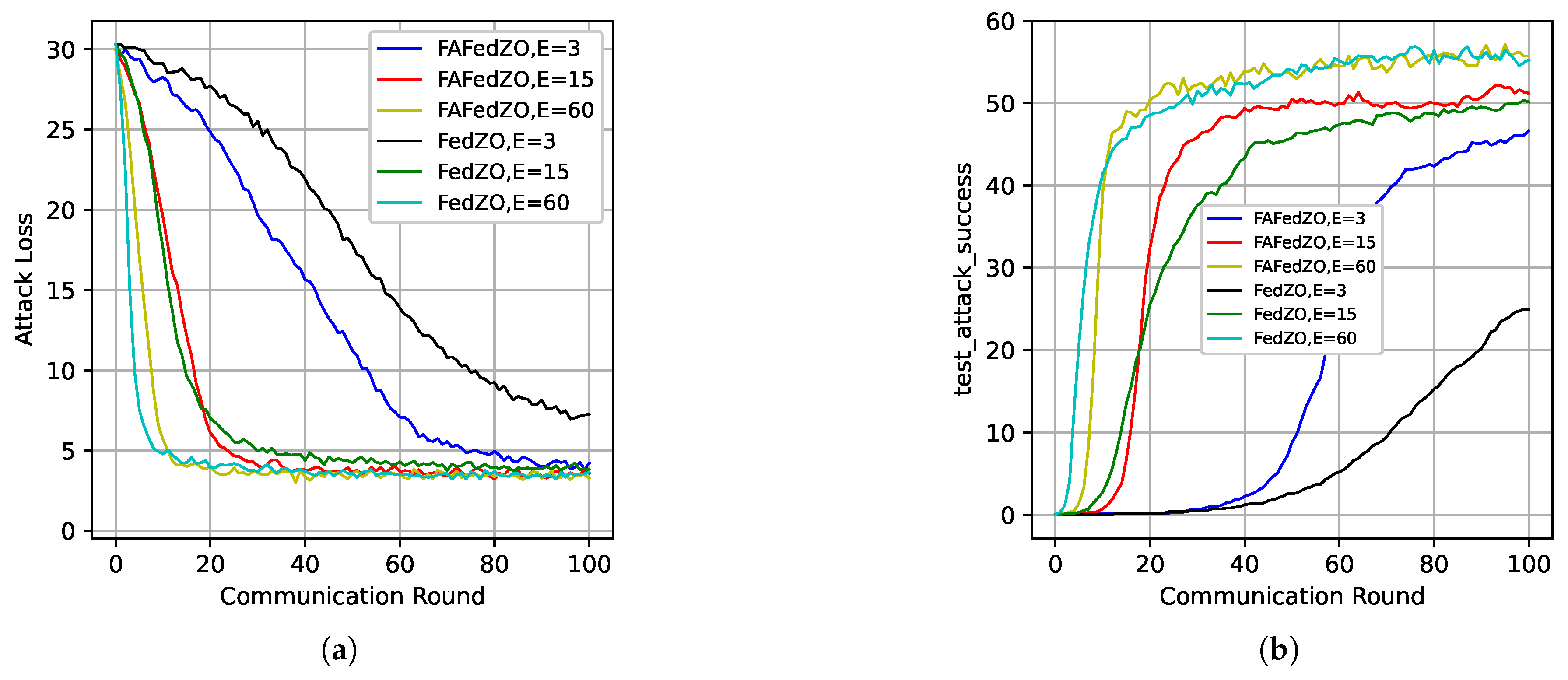
In addition, we also discuss the performance of our algorithm under the setting of non-Independent and Identically Distributed (non-IID) data.

Figure 7 presents the impact of the number of local updates on the attack loss and accuracy of the algorithm under the non-IID setting. It can be observed that, compared with Figure 2a,d, the attack accuracy in this case is lower than that under the IID setting, which is attributed to the influence of the non-IID setting and aligns with our expectations. Furthermore, the results also indicate that under the non-IID setting, the performance of the FAFedZO algorithm remains superior to that of the FedZO algorithm, and both achieve comparable performance levels when $E=60$.

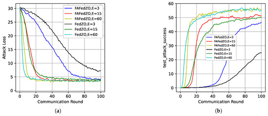
Figure 7. The impact of different numbers of local updates when selecting $Q=50$ and $M=30$ in a non-IID setting. (a) Attack loss; (b) Testing accuracy.

The conclusions we previously mentioned are also supported by Figure 8 and Figure 9. Therefore, in summary, the FAFedZO algorithm demonstrates superior performance in both IID and non-IID environments.

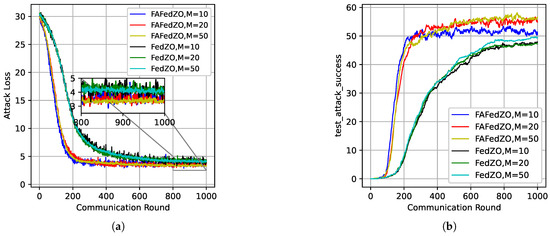
Figure 8. The impact of the number of participating edge devices when selecting $Q=50$ and $E=1$ under the non-IID setting. (a) Attack loss; (b) Testing accuracy.

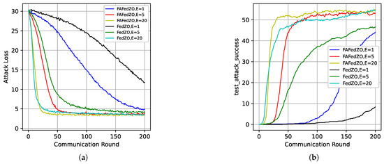
Figure 9. The impact of different numbers of local updates when selecting $Q=50$ and $M=50$ under the non-IID setting. (a) Attack loss; (b) Testing accuracy.

6. Conclusions

In this paper, we proposed FAFedZO, a federated optimization algorithm that combines derivative-free zero-order optimization with an adaptive method. We conducted a theoretical analysis of the algorithm to prove its convergence and presented the computational complexity and convergence rate of the FAFedZO algorithm. Finally, we conducted a large number of comparative experiments on the MNIST, CIFAR-10, and Fashion-MNIST datasets. The results demonstrate that our method can achieve a faster convergence rate compared to general zero-order optimization algorithms, verifying the effectiveness of the algorithm proposed in this paper.

References

- McMahan, B.; Moore, E.; Ramage, D.; Hampson, S.; y Arcas, B.A. Communication-efficient learning of deep networks from decentralized data. In Proceedings of the Artificial Intelligence and Statistics, Fort Lauderdale, FL, USA, 20–22 April 2017; pp. 1273–1282. [Google Scholar]
- Shi, Y.; Yang, K.; Yang, Z.; Zhou, Y. Mobile Edge Artificial Intelligence: Opportunities and Challenges; Elsevier: Amsterdam, The Netherlands, 2021. [Google Scholar]
- Yang, L.; Tan, B.; Zheng, V.W.; Chen, K.; Yang, Q. Federated recommendation systems. In Federated Learning: Privacy and Incentive; Springer International Publishing: Cham, Switzerland, 2020; pp. 225–239. [Google Scholar]
- Yang, K.; Shi, Y.; Zhou, Y.; Yang, Z.; Fu, L.; Chen, W. Federated machine learning for intelligent IoT via reconfigurable intelligent surface. IEEE Netw. 2020, 34, 16–22. [Google Scholar]
- Tian, J.; Smith, J.S.; Kira, Z. Fedfor: Stateless heterogeneous federated learning with first-order regularization. arXiv 2022, arXiv:2209.10537. [Google Scholar]
- Zhang, M.; Sapra, K.; Fidler, S.; Yeung, S.; Alvarez, J.M. Personalized federated learning with first order model optimization. arXiv 2021, arXiv:2012.08565. [Google Scholar]
- Elbakary, A.; Issaid, C.B.; Shehab, M.; Seddik, K.G.; ElBatt, T.A.; Bennis, M. Fed-Sophia: A Communication-Efficient Second-Order Federated Learning Algorithm. arXiv 2024, arXiv:2406.06655. [Google Scholar]
- Dai, Z.; Low, B.K.H.; Jaillet, P. Federated Bayesian optimization via Thompson sampling. Adv. Neural Inf. Process. Syst. 2020, 33, 9687–9699. [Google Scholar]
- Staib, M.; Reddi, S.; Kale, S.; Kumar, S.; Sra, S. Escaping saddle points with adaptive gradient methods. In Proceedings of the International Conference on Machine Learning, Long Beach, CA, USA, 10–15 June 2019; pp. 5956–5965. [Google Scholar]
- Chen, X.; Li, X.; Li, P. Toward communication efficient adaptive gradient method. In Proceedings of the 2020 ACM-IMS on Foundations of Data Science Conference, San Francisco, CA, USA, 18–20 October 2020; pp. 119–128. [Google Scholar]
- Reddi, S.; Charles, Z.; Zaheer, M.; Garrett, Z.; Rush, K.; Konečnỳ, J.; Kumar, S.; McMahan, H.B. Adaptive federated optimization. arXiv 2020, arXiv:2003.00295. [Google Scholar]
- Wang, Y.; Lin, L.; Chen, J. Communication-efficient adaptive federated learning. In Proceedings of the International Conference on Machine Learning, Baltimore, MD, USA, 17–23 July 2022; pp. 22802–22838. [Google Scholar]
- Zhang, P.; Yang, X.; Chen, Z. Neural network gain scheduling design for large envelope curve flight control law. J. Beijing Univ. Aeronaut. Astronaut. 2005, 31, 604–608. [Google Scholar]
- Wang, J.; Liu, Q.; Liang, H.; Joshi, G.; Poor, H.V. A novel framework for the analysis and design of heterogeneous federated learning. IEEE Trans. Signal Process. 2021, 69, 5234–5249. [Google Scholar]
- Li, T.; Sahu, A.K.; Zaheer, M.; Sanjabi, M.; Talwalkar, A.; Smith, V. Federated optimization in heterogeneous networks. Proc. Mach. Learn. Syst. 2020, 2, 429–450. [Google Scholar]
- Karimireddy, S.P.; Kale, S.; Mohri, M.; Reddi, S.; Stich, S.; Suresh, A.T. Scaffold: Stochastic controlled averaging for federated learning. In Proceedings of the International Conference on Machine Learning, Virtual, 13–18 July 2020; pp. 5132–5143. [Google Scholar]
- Pathak, R.; Wainwright, M.J. FedSplit: An algorithmic framework for fast federated optimization. Adv. Neural Inf. Process. Syst. 2020, 33, 7057–7066. [Google Scholar]
- Zhang, X.; Hong, M.; Dhople, S.; Yin, W.; Liu, Y. Fedpd: A federated learning framework with adaptivity to non-IID data. IEEE Trans. Signal Process. 2021, 69, 6055–6070. [Google Scholar]
- Wang, S.; Roosta, F.; Xu, P.; Mahoney, M.W. Giant: Globally improved approximate newton method for distributed optimization. Adv. Neural Inf. Process. Syst. 2018, 31, 2332–2342. [Google Scholar]
- Li, T.; Sahu, A.K.; Zaheer, M.; Sanjabi, M.; Talwalkar, A.; Smithy, V. Feddane: A federated newton-type method. In Proceedings of the 2019 53rd Asilomar Conference on Signals, Systems, and Computers , Pacific Grove, CA, USA, 3–6 November 2019; pp. 1227–1231. [Google Scholar]
- Xu, A.; Huang, H. Coordinating momenta for cross-silo federated learning. In Proceedings of the AAAI Conference on Artificial Intelligence, Online, 22 February–1 March 2022; Volume 36, pp. 8735–8743. [Google Scholar]
- Das, R.; Acharya, A.; Hashemi, A.; Sanghavi, S.; Dhillon, I.S.; Topcu, U. Faster non-convex federated learning via global and local momentum. In Proceedings of the Uncertainty in Artificial Intelligence, Eindhoven, The Netherlands, 1–5 August 2022; pp. 496–506. [Google Scholar]
- Khanduri, P.; Sharma, P.; Yang, H.; Hong, M.; Liu, J.; Rajawat, K.; Varshney, P. Stem: A stochastic two-sided momentum algorithm achieving near-optimal sample and communication complexities for federated learning. Adv. Neural Inf. Process. Syst. 2021, 34, 6050–6061. [Google Scholar]
- Tang, Y.; Zhang, J.; Li, N. Distributed zero-order algorithms for nonconvex multiagent optimization. IEEE Trans. Control Netw. Syst. 2020, 8, 269–281. [Google Scholar]
- Nikolakakis, K.; Haddadpour, F.; Kalogerias, D.; Karbasi, A. Black-box generalization: Stability of zeroth-order learning. Adv. Neural Inf. Process. Syst. 2022, 35, 31525–31541. [Google Scholar]
- Balasubramanian, K.; Ghadimi, S. Zeroth-order (non)-convex stochastic optimization via conditional gradient and gradient updates. Adv. Neural Inf. Process. Syst. 2018, 31, 3459–3468. [Google Scholar]
- Fang, W.; Yu, Z.; Jiang, Y.; Shi, Y.; Jones, C.N.; Zhou, Y. Communication-efficient stochastic zeroth-order optimization for federated learning. IEEE Trans. Signal Process. 2022, 70, 5058–5073. [Google Scholar]
- Li, Z.; Ying, B.; Liu, Z.; Yang, H. Achieving Dimension-Free Communication in Federated Learning via Zeroth-Order Optimization. arXiv 2024, arXiv:2405.15861. [Google Scholar]
- Maritan, A.; Dey, S.; Schenato, L. FedZeN: Quadratic convergence in zeroth-order federated learning via incremental Hessian estimation. In Proceedings of the 2024 European Control Conference, Stockholm, Sweden, 25–28 June 2024; pp. 2320–2327. [Google Scholar]
- Mhanna, E.; Assaad, M. Rendering wireless environments useful for gradient estimators: A zero-order stochastic federated learning method. In Proceedings of the 2024 60th Annual Allerton Conference on Communication, Control, and Computing, Urbana, IL, USA, 24–27 September 2024; IEEE: New York, NY, USA, 2024; pp. 1–8. [Google Scholar]
- Diederik, P.K. Adam: A method for stochastic optimization. arXiv 2014, arXiv:1412.6980. [Google Scholar]
- Duchi, J.; Hazan, E.; Singer, Y. Adaptive subgradient methods for online learning and stochastic optimization. J. Mach. Learn. Res. 2011, 12, 2121–2159. [Google Scholar]
- Ling, X.; Fu, J.; Wang, K.; Liu, H.; Chen, Z. Ali-dpfl: Differentially private federated learning with adaptive local iterations. In Proceedings of the 2024 IEEE 25th International Symposium on a World of Wireless, Mobile and Multimedia Networks, Perth, Australia, 4–7 June 2024; pp. 349–358. [Google Scholar]
- Cong, Y.; Qiu, J.; Zhang, K.; Fang, Z.; Gao, C.; Su, S.; Tian, Z. Ada-FFL: Adaptive computing fairness federated learning. CAAI Trans. Intell. Technol. 2024, 9, 573–584. [Google Scholar]
- Huang, Y.; Zhu, S.; Chen, W.; Huang, Z. FedAFR: Enhancing Federated Learning with adaptive feature reconstruction. Comput. Commun. 2024, 214, 215–222. [Google Scholar]
- Li, Y.; He, Z.; Gu, X.; Xu, H.; Ren, S. AFedAvg: Communication-efficient federated learning aggregation with adaptive communication frequency and gradient sparse. J. Exp. Theor. Artif. Intell. 2024, 36, 47–69. [Google Scholar]
- Yi, X.; Zhang, S.; Yang, T.; Johansson, K.H. Zeroth-order algorithms for stochastic distributed nonconvex optimization. Automatica 2022, 142, 110353. [Google Scholar]
- Wu, X.; Huang, F.; Hu, Z.; Huang, H. Faster adaptive federated learning. In Proceedings of the AAAI Conference on Artificial Intelligence, Vancouver, BC, Canada, 20–27 February 2023; Volume 37, pp. 10379–10387. [Google Scholar]
- Gao, X.; Jiang, B.; Zhang, S. On the information-adaptive variants of the ADMM: An iteration complexity perspective. J. Sci. Comput. 2018, 76, 327–363. [Google Scholar]
Disclaimer/Publisher’s Note: The statements, opinions and data contained in all publications are solely those of the individual author(s) and contributor(s) and not of MDPI and/or the editor(s). MDPI and/or the editor(s) disclaim responsibility for any injury to people or property resulting from any ideas, methods, instructions or products referred to in the content. |
© 2025 by the authors. Licensee MDPI, Basel, Switzerland. This article is an open access article distributed under the terms and conditions of the Creative Commons Attribution (CC BY) license (https://creativecommons.org/licenses/by/4.0/).