Abstract
To mitigate the limited accuracy of the Simplified General Perturbations 4 (SGP4) model in predicting medium-orbit satellite trajectories, we propose an enhanced methodology integrating deep learning with traditional algorithms. The developed BiLSTM-TS forecasting framework comprises a Bidirectional Long Short-Term Memory (BiLSTM) network, trend analysis module (T), and seasonal decomposition module (S). This architecture effectively captures sequential dependencies, trend variations, and periodic patterns within time series data, thereby improving prediction interpretability. In our experimental validation, we chose Beidou-2 M6 (C14), GSAT0203 (GALILEO 7), and the Global Positioning System (GPS) satellite named GPS BIIR-13 (PRN 02) as representative satellites. Satellite position data derived from conventional orbital models were input into the BiLSTM-TS framework for statistical learning to predict orbital deviations. These predicted errors were subsequently combined with SGP4 model outputs obtained through Two-Line Element set (TLE) data analysis to minimize overall trajectory inaccuracies. Using BeiDou-2 M6 (C14) as a case study, results indicated that the BiLSTM-TS implementation achieved significant error reduction; mean-squared error along the X-axis was reduced to 0.0309 km2, with mean absolute error of 0.1245 km, and maximum absolute error was constrained to 0.4448 km.
1. Introduction
Medium-Earth orbit (MEO) is the orbital region between about 2000 km and 35,786 km above the Earth’s surface and is commonly used for navigation, communication, and scientific exploration satellites. Compared with low-orbit satellites, medium-orbit satellites are higher in altitude, cover a wider range, and provide better communication performance without reaching the orbital altitude of high-orbit satellites, so they are widely used in the construction of global navigation satellite systems (GNSSs). For example, the satellites belonging to GPS, BeiDou, Galileo, and other GNSSs belong to this orbit. The study of the orbit accuracy of MEO satellites helps to guarantee navigation and positioning accuracy, enhance satellite life and mission efficiency, provide high-quality data and information, and is also conducive to the monitoring and control of satellites and the advancement of space technology. GNSS has become the most widely used navigation method, providing users with positioning and navigation timing (PNT) services in various applications [1].
Real-time monitoring, tracking, cataloguing and comparison of space targets, orbital prediction and collision warning are important aspects of maintaining the safety of the space environment [2,3].
In the area of space target monitoring and identification, Guo et al. introduced an enhanced spatial debris detection method based on You Only Look Once: Unified, Real-Time Object Detection (YOLOv8), which improves the detection accuracy and processing speed of the model by incorporating a cross-scale feature fusion module into the neck network and fine-tuning the feature fusion component [4]. Cheng et al. proposed a design architecture of a twin control system for space object detection equipment and verified it with a gimbal model. The system architecture can reduce the observation limitations and improve the observation efficiency [5]. Guo et al. propose a method of constructing an evaluation model for the coordinated detection system of space objects by applying fuzzy theory. By establishing a system evaluation index system, constructing a Combined Modeling of Genetic Algorithms (GA) and Backpropagation Neural Networks (BP) effectiveness evaluation meta-model, and adopting a fuzzy evaluation method and the principle of maximum affiliation, the purpose of improving the accuracy and sensitivity of the judging model is achieved [6].
Currently, there are three types of methods applied to improve the accuracy of orbital forecasts: more accurate forecast models, more precise data features as inputs (e.g., atmospheric drag coefficients, solar pressure, etc.) [7,8,9,10], and corrections to the TLE data themselves or to their analytical results. TLE data, as the public data in the field of aerospace, store a large amount of orbital information. By learning the TLE data to obtain the flat root number and applying it to orbit prediction, the cumulative error of long-term prediction can be reduced, and by analyzing the TLE data to obtain the relevant information of satellite position through the SGP4 model, and predicting the parsing error of the TLE data through deep learning or other methods, the purpose of correcting the error of orbit prediction and improving the accuracy of orbit prediction can be achieved [11].
Forecasting models are categorized into analytical [12,13], semi-analytical [14], and numerical [15] depending on their forecasting methods, where analytical methods are suitable for simple environments and have high efficiency but average accuracy, and numerical methods have high accuracy but low efficiency. In order to balance the relationship between efficiency and accuracy, researchers take the semi-analytical method, which has relatively high accuracy and efficiency, as a research hotspot.
Common prediction models include the two-body model, J2 perturbation model, SGP4 model, and High-Precision Orbit Propagator (HPOP) model. Among them, the orbital mechanics method applied by the two-body model and the J2 perturbation model belong to the analytical method, SGP4 belongs to the semi-analytical method, and HPOP belongs to the numerical method. Selecting a higher-accuracy prediction model can improve the orbit prediction accuracy, but its prediction efficiency may be degraded.
Among the factors affecting the orbit prediction accuracy, the atmospheric drag coefficient and solar air pressure are more important parameters, and the researchers can effectively improve the orbit prediction accuracy by applying the atmospheric drag coefficient or solar air pressure obtained from the model prediction to the orbit prediction model mentioned above, replacing the original fixed value.
In addition, with the rapid development of deep learning models, researchers have carried out many studies from the perspective of deep learning models. Given the time-series characteristics of space target orbit data, studying the time-series prediction problem can effectively achieve the purpose of space target orbit forecasting. Ji et al. enhanced arc depression prediction by integrating convolutional neural network (CNN), long and short-term memory network (LSTM), and attentional mechanism, and utilized Adaptive Rabbit Optimization Algorithm (AROA) for the first time to perform control law accelerator (CLA) parameter tuning. This combination improves the predictive performance and generalization ability of the model. By effectively utilizing historical data and demonstrating superior time series processing capabilities, the AROA-CLA model exhibits excellent prediction accuracy and stability over different time scales [16]. By investigating the combination of LSTM and BP neural network, Guo et al. improved the stability of the model, while the forecasting accuracy was effectively enhanced [17]. Cao et al. proposed a multivariate time series prediction method based on a convolutional–residual gated recursive hybrid model (CNN-DA-RGRU), which employs a two-layer attentional mechanism to address the spatial feature extraction and time-varying mining of historical sequence data [18].
Yang et al. proposed a continuous variational pattern decomposition based on SBOA optimization to extract the predictable components of load sequences and introduced a combined prediction structure of temporal convolutional networks (TCNs) and BiLSTM networks to mine each load component’s temporal characteristics to obtain short-term load prediction results [19]. Zhong et al. proposed a combined model based on the attention-based dynamic internal partial least squares (DiPLS) model and BiLSTM model for solar power prediction [20]. Zhou et al. proposed a complementary integrated empirical mode decomposition based on Bayesian optimization algorithm and data differential processing (CEEMD) and LSTM short-term air traffic flow prediction model to achieve improved accuracy in short-term air traffic flow prediction [21]. Deep learning models have become a research hotspot in various industries, and the combination of temporal prediction and deep learning is constantly deepening.
In the space domain, deep learning and time series prediction remain important. Liu et al. proposed a two-step graphical convolutional neural network (TS-GCN) framework considering skewed data and dimensionality integrating resampling and streamlining architectures, and applying to a specific satellite model yielded 98.93% state identification and 99.13% prediction accuracy [22]. Yang et al. proposed a new multi-task-based learning time-series anomaly detection (MTAD) method that facilitates anomaly detection by capturing spatio-temporal correlation of data to learn generalized normal patterns, which was revealed to be superior to existing techniques through the application of a real spacecraft dataset, and further ablation tests for each task demonstrated the effectiveness of fusing multiple tasks [23]. Sunspots are an important indicator of the solar activity cycle, and their number and distribution can reflect changes in the Sun’s magnetic activity and solar cycle, which have a significant impact on satellite orbits and space missions. The number and distribution of sunspots belong to time series data, and the study of their trends and periodicity is conducive to grasping the anomalies of satellite orbits. Chen et al. developed a hybrid model consisting of a one-dimensional convolutional neural network (1D-CNN) for extracting sunspot features and a BiLSTM embedded in a multi-head attention mechanism (MHAM) to learn the intrinsic relationship between the data and ultimately predict the sunspot number [24].
In this paper, a deep learning prediction model based on BiLSTM-TS is proposed from the parsing results of TLE data. The model improves the orbit prediction accuracy by combining the parsed data with the SGP4 model and learning the satellite time series data information: position error, velocity and acceleration to realize the prediction of future orbit error.
2. Materials and Methods
In this study, we introduce the BiLSTM-TS model, an innovative approach designed for forecasting time series data from mid-orbit satellites. This model enhances the traditional BiLSTM framework by incorporating two specialized components: a Trend Block (T) and a Season Block (S). At the heart of the BiLSTM-TS model lies the BiLSTM Network, which serves as the cornerstone for time-series modeling and feature extraction. Its primary function is to adeptly capture long-term dependencies within the time series data.
Time series data often exhibit patterns that extend across numerous time steps. The BiLSTM network, with its unique architecture, is particularly well-suited to identify and leverage these long-term dependencies. It achieves this by harnessing both forward and backward hidden states, enabling it to process information from both the start and the end of the sequence. This bidirectional approach allows the BiLSTM to assimilate a richer context than would be possible by considering only unidirectional sequence data. The hidden states produced by the BiLSTM at each time step are subsequently utilized by the Trend and Season Blocks to discern and extract underlying long-term trends and periodic fluctuations, respectively. This comprehensive analysis facilitated by the BiLSTM-TS model ensures a more nuanced and accurate forecasting of satellite time series data.
The Trend Block is designed to capture the long-term trend of the time series by utilizing the output from the final time step of the BiLSTM. To enhance its effectiveness, an attention mechanism is employed to assign weights to each time step of the BiLSTM output, thereby focusing on the most critical aspects and generating a context vector. This vector is then input into the Trend Block to facilitate further trend prediction.
On the other hand, the Season Block leverages the outputs from all time steps of the BiLSTM. This approach is adopted because periodic fluctuations can manifest at any point within the sequence, and utilizing the complete time series information allows for a more effective extraction of local periodic features. The outputs from each time step are processed through a convolutional layer, where multi-scale convolutional operations are applied to extract periodic features. This method aids the model in comprehending the short-term fluctuations present in the time series.
For the empirical analysis in this study, Standard Product 3 (SP3) precise ephemeris files, complemented by TLE data, were selected. These files are read and converted into a time series data format, with updates occurring every five minutes. In the forecasting process, the model employs univariate or multivariate rolling forecasts to predict future data points, ensuring a comprehensive and robust forecasting capability.
2.1. Dataset
The GNSS represents a class of satellite systems designed to deliver navigation, positioning, and timing information on both global and regional scales. This comprehensive system includes not only global constellations such as the United States’ GPS, Russia’s GLOBAL NAVIGATION SATELLITE SYSTEM (GLONASS), the European Union’s Galileo, and China’s BeiDou, but also regional systems like Japan’s Quasi-Zenith Satellite System (QZSS) and India’s Indian Regional Navigation Satellite System (IRNSS), alongside augmentation systems such as the United States’ Wide Area Augmentation System (WAAS), Europe’s European Geostationary Navigation Overlay Service (EGNOS), and Japan’s Multi-Functional Satellite Augmentation System (MSAS). By harnessing its high-precision positioning and navigation capabilities, GNSS finds extensive applications in agriculture, military operations, transportation, mobile device positioning, and beyond. Furthermore, MEO satellites contribute significantly to communication, meteorological monitoring, environmental surveillance, scientific exploration, and research endeavors [25,26].
As depicted in Table 1, navigation satellites from various systems display distinct orbital periods, inclinations, and altitudes. To ensure the experiment’s broad applicability, this study focuses on three satellites: GPS BIIR-13 (PRN 02), BeiDou-2 M6 (C14), and GSAT0203 (GALILEO 7). These satellites aptly exemplify the orbital characteristics of MEO satellites across different systems. The North American Aerospace Defense Command (NORAD) assigns a unique number to each of the cataloged satellites.

Table 1.
Global positioning and navigation system satellite sample information table.
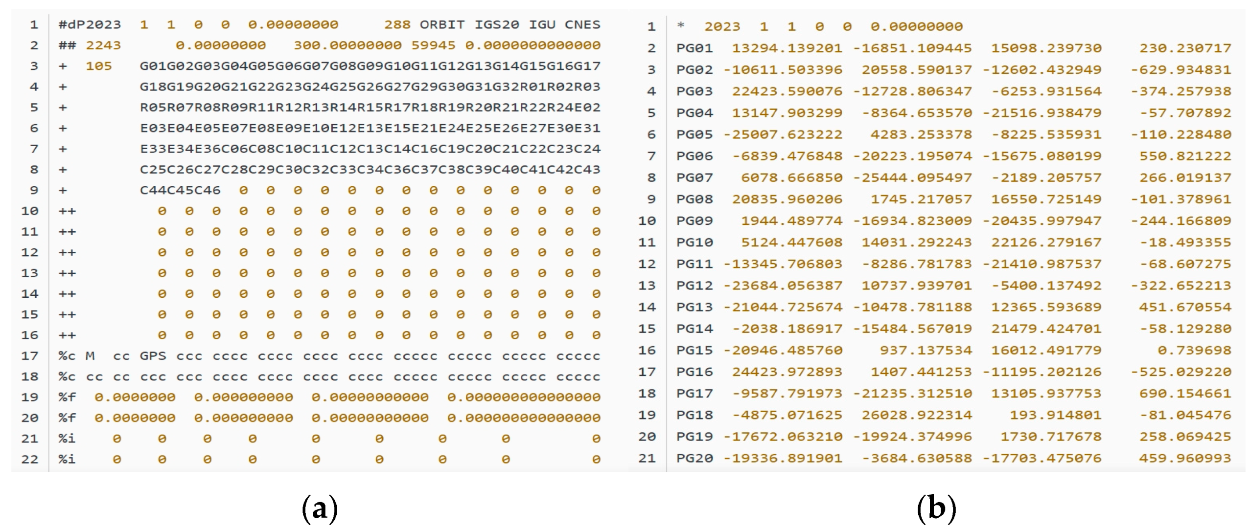
This study utilizes SP3 precise ephemeris data and TLE data related to MEO satellites. The SP3 precise ephemeris data are primarily sourced from global and regional GNSS service agencies, as well as research institutions. Key providers of SP3 files include the International GNSS Service (IGS), regional GNSS service organizations, and various academic and research institutions. The SP3 precise ephemeris file, which is presented in a textual format, is illustrated in Figure 1. The TLE data, acquired from the Space-Track website, consist of formatted data that describe the position and motion of artificial satellites orbiting the Earth. These data are widely used for trajectory prediction, space object monitoring, and satellite tracking. The structure of the TLE data is shown in Figure 2. Together, these datasets provide a comprehensive foundation for the analysis and forecasting tasks undertaken in this research. Precision ephemeris is an after-the-fact ephemeris, which is highly accurate and can be regarded as the real coordinates of satellites, but because of the time lag, it cannot meet the real-time requirements. In the satellite orbit prediction experiment, the precision ephemeris data information as the real value meets the accuracy requirements of this paper.
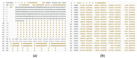
Figure 1.
(a) Header information format of SP3 precise ephemeris file; (b) SP3 precise ephemeris file format.

Figure 2.
TLE data text format.
The header section of the SP3 precise ephemeris file primarily offers essential metadata and parsing guidelines, encompassing details such as the file version, temporal coverage, ephemeris interval, the number of satellites, and their respective identifiers (e.g., GPS, GLONASS, BeiDou, etc.). The body of the file, on the other hand, contains detailed positional data for each satellite, along with clock offset information. The positional data are defined within the Earth-Centered, Earth-Fixed (ECEF) coordinate system and include three-dimensional coordinates (X, Y, Z) for precise satellite positioning. This structured format ensures comprehensive and accurate representation of satellite trajectories and timing information.
TLE data encapsulate critical orbital parameters of a satellite and are typically represented in a two-line textual format. The first line contains essential details such as the satellite’s catalog number, international designator (comprising the launch year and sequence number), orbital inclination, right ascension of the ascending node, orbital eccentricity, argument of perigee, mean anomaly, and mean motion. The second line provides additional parameters, including the satellite’s mean motion derivative, second derivative of mean motion, BSTAR drag term, and epoch time. These elements collectively describe the satellite’s orbital characteristics and motion.
In certain research contexts, TLE data are treated as empirical observations of a satellite’s position [27,28]. This approach leverages the TLE’s comprehensive orbital information to approximate the satellite’s actual trajectory, making it a valuable resource for applications such as orbit prediction, space object tracking, and collision avoidance analysis.
2.2. Data Preprocessing
Since the positional data in the SP3 precise ephemeris file are expressed in the ECEF coordinate system, while the satellite position coordinates derived from TLE data using the SGP4 model are established in the True Equator, Mean Equinox (TEME) coordinate system, it is necessary to convert the ECEF coordinate system into the TEME coordinate system to unify the reference frames. The conversion formula is as follows:
where is the angle of rotation of the Earth with respect to the geocentric inertial coordinate system, is Greenwich Mean Time, is the correction due to chapter motion and polar shift, is the matrix of rotation about the z-axis, is the matrix of rotation about the y-axis, represents the rotation angle around the z-axis. , and are the age difference angles, is the angle of intersection of the yellows and equinoxes, is the change in the declination of the ruddy longitude due to the chapter motion, is the matrix of the chapter motion, is the matrix of the age difference, and is the coordinates in the geocentric inertial system. Therefore, the complete transformation formula is as follows:
After processing the data, the three-axis position error, velocity magnitude, and acceleration information of the satellite at a specific moment can be obtained.
Once the data are loaded from an external file, the BiLSTM-TS model can extract key variables such as axial error, axial velocity, and axial acceleration. These variables represent the target features of interest in the time series. To ensure consistency and avoid the influence of varying feature scales during training, the data must be normalized to a range of [0, 1].
The raw data are then transformed into sequence data with a fixed time window length. This fixed time window helps extract temporal features, ensures input data consistency, and enhances the model’s ability to adapt to data from different time periods, thereby improving its generalization capability.
2.3. Prediction Process
The deep learning model is designed to correct forecasting errors from traditional models, with the SGP4 model selected as the traditional approach for parsing TLE data. The SGP4 model, a widely adopted method for predicting artificial satellite orbits, is based on general perturbation theory and has been extensively used for tasks such as forecasting satellite positional trajectories and calculating satellite transit times.
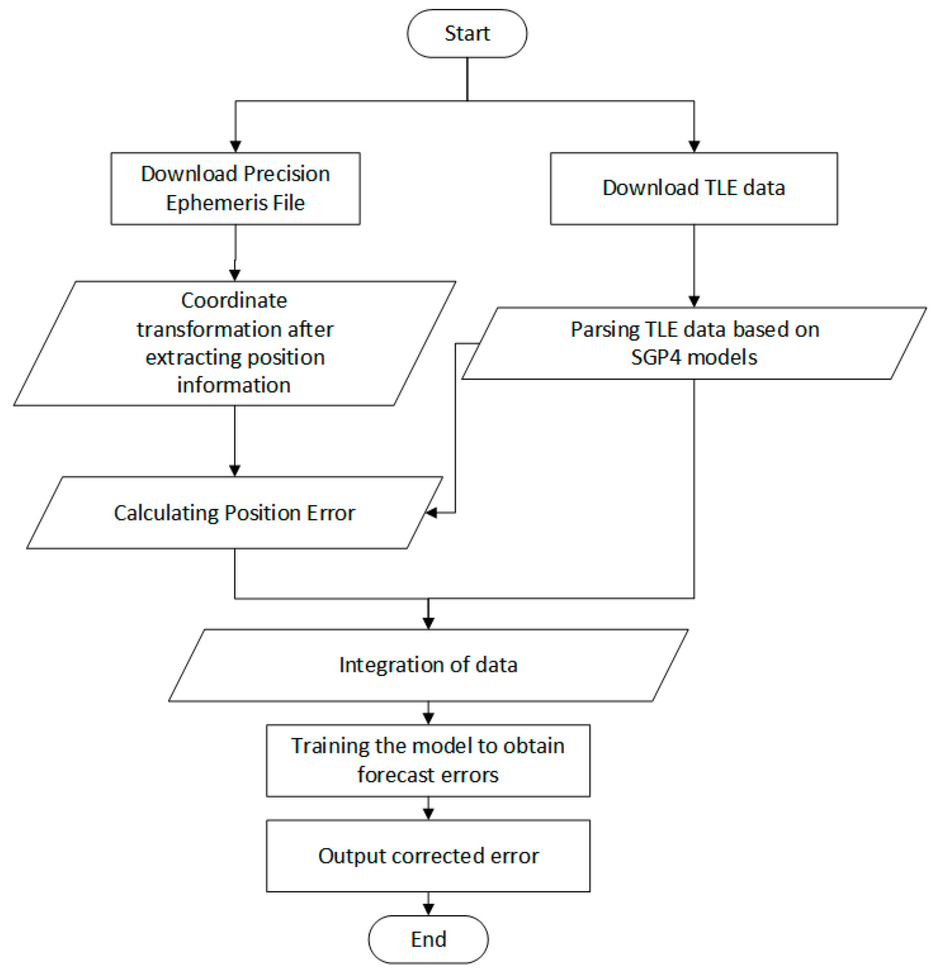
The data span from 16 December 2023 to 26 December 2023. The most recent TLE data published each day are utilized to predict the satellite-related information for the following day. Error data, velocity information, and acceleration from 17 December 2023 to 26 December 2023 serve as inputs to the deep learning model, enabling the forecasting of the satellite’s position information for 27 December 2023—a one-day-ahead prediction. The error data are derived from the difference between the parsed results of the SP3 precise ephemeris file and the SGP4 model’s output, with the SP3 file’s stored data considered the real value. The overall process of trajectory forecasting is illustrated in Figure 3.
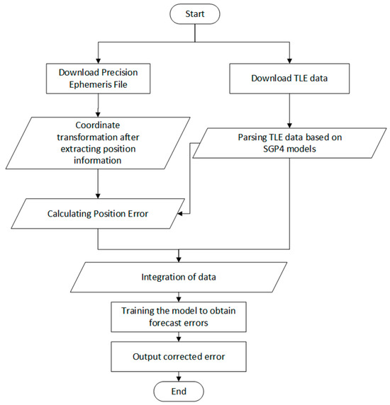
Figure 3.
The entire process of orbital forecasting, from data download to result output.
The forecasting process is roughly divided into four parts: data download, data preprocessing, model training, and correction of forecast results.
2.4. Prediction Model
The BiLSTM-TS model integrates a BiLSTM architecture with specialized trend and season blocks.
The BiLSTM excels at capturing long-term dependencies in time series data by leveraging both past and future information through its bidirectional structure, thereby enhancing the model’s contextual understanding of the sequence.
The trend block is designed to extract long-term trend components from the sequence, which are progressively mapped to the output via a fully connected layer, enabling it to handle smoothly evolving trends in the time series. Meanwhile, the season block employs multi-scale convolutional operations to capture periodic features, utilizing convolutional kernels of varying sizes to extract both short-term and long-term periodic fluctuations, providing a more comprehensive understanding of cyclical patterns in the data.
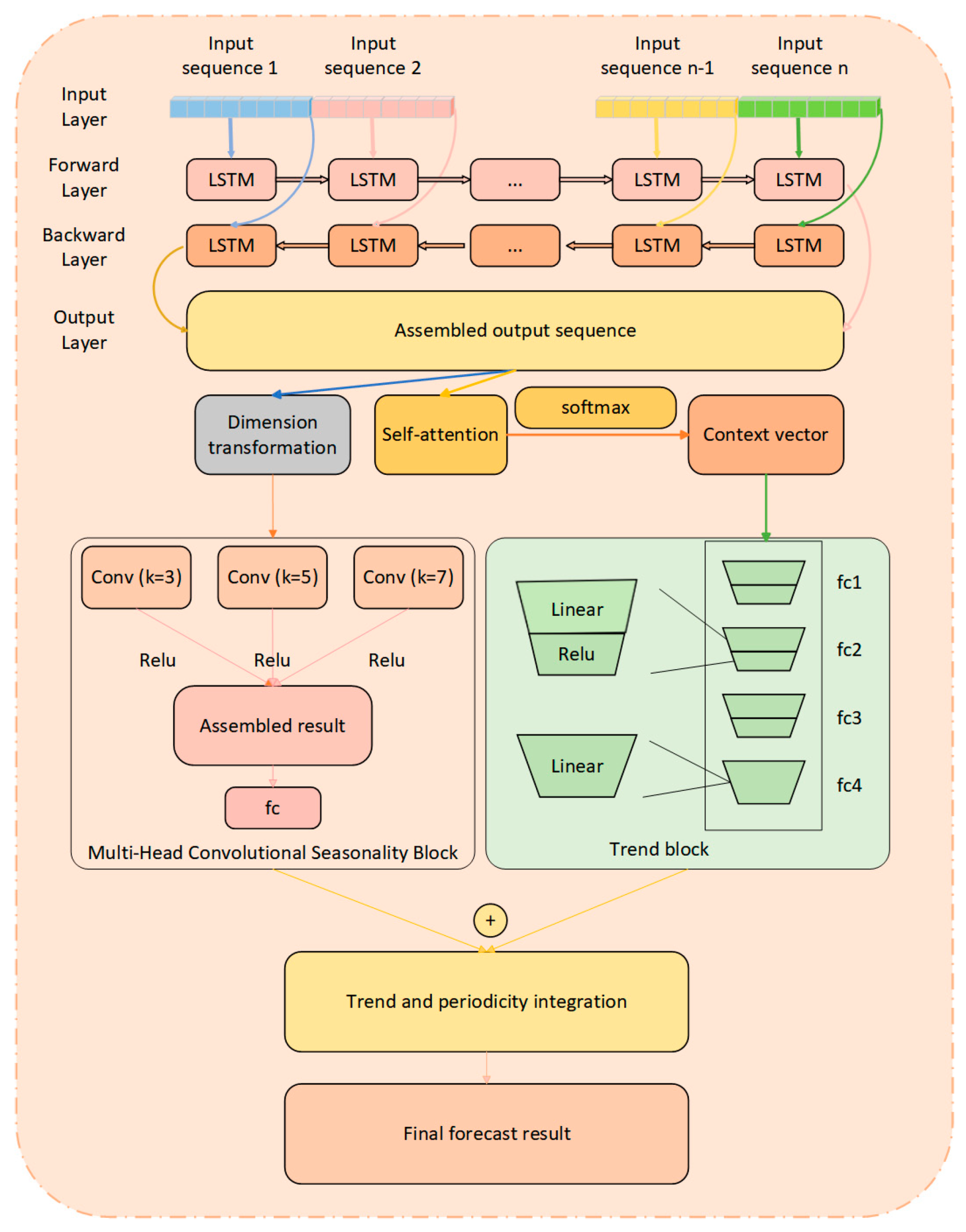
By combining these three components, the model not only effectively learns trend changes and periodic patterns in the time series but also extracts features at multiple levels and scales. This approach enhances prediction accuracy and robustness, particularly when dealing with complex and variable time series data. Additionally, it improves the model’s generalization capabilities and increases its interpretability. The structure of the BiLSTM-TS model is illustrated in Figure 4.
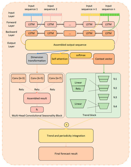
Figure 4.
BiLSTM-TS model structure diagram.
BiLSTM serves as the core of the whole model and contains forward LSTM and reverse LSTM.
Forward LSTM: Given an input sequence ,,…,, the forward LSTM is computed as follows:
where denotes the sigmoid activation function and denotes the hyperbolic tangent activation function. , , , and denote the input gate, forgetting gate, output gate, and candidate memory cell, respectively. is the hidden state at the -th time step and is the cell state. , , , denote the weighting matrix, and , , , denote the bias vector. represents the hidden state of the previous moment () stitched together with the input of the current moment ().
Reverse LSTM: The computation of reverse LSTM is similar to forward except that the computation is performed in reverse at the time step.
Output of BiLSTM: For each time step , the output of BiLSTM is a splice of forward and reverse hidden states.
where is the output of the forward LSTM and is the output of the reverse LSTM. denotes the output vector spliced from the hidden state () of the forward LSTM and the hidden state () of the backward LSTM at moment t.
Attention Mechanism:
In the model, the purpose of the attention mechanism is to weight the LSTM outputs of all time steps by calculating the attention weights of each time step to generate a weighted context vector.
where is the attention score at the -th time step and is the weight matrix. is the attention weight of the -th time step and denotes the attention to that time step.
Calculate the context vector by weighted sum:
Trend Block (Figure 5):
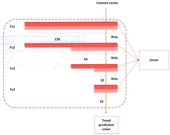
Figure 5.
Four-layer fully connected trend block structure.
The Trend Block is designed to capture long-term trend patterns in time series data. This module first generates a globally aware context vector through an attention mechanism, then employs a multi-layer perceptron (MLP) architecture for deep trend feature extraction. Specifically, it processes the context vector derived from BiLSTM outputs through a four-layer fully connected network:
- Input layer maps features to 128-dimensional space.
- Second layer compresses representations to 64 dimensions.
- Third layer refines features to 32 key dimensions.
- Output layer generates final trend predictions.
The complete formula for the trend block is as follows:
where , , , and , , , are the weights and biases of the trend block. is the activation function, which is used to introduce the nonlinear. And denotes the output vector of the fully connected layer.
Season Block (Multiple Convolution):
From Figure 6, it can be observed that the architectural design of the multi-scale convolutional seasonality block is presented. This module specializes in detecting and modeling periodic patterns within time series data through a hierarchical processing pipeline. Operating on the BiLSTM outputs, it employs parallel convolutional streams with varying kernel dimensions (3-, 5-, and 7-unit spans) to concurrently capture short-term oscillations and extended cyclical variations. The processing pipeline comprises three key stages:
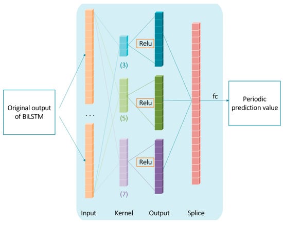
Figure 6.
Three-scale multi-headed convolutional seasonality block architecture.
Multi-scale Feature Extraction: Three independent convolutional operations with distinct receptive fields isolate periodic signatures at different temporal resolutions.
Feature Fusion: Concatenated outputs from parallel convolutions create enriched multi-frequency representations.
Dimensionality Projection: A final fully connected layer synthesizes the integrated features into interpretable periodic components.
This design enables simultaneous detection of immediate fluctuations (e.g., orbital perturbation cycles) and long-term periodicities (e.g., seasonal orbital variations), while dropout regularization enhances model generalizability. Multi-scale feature extraction can effectively improve model performance and has been applied to a variety of fields [29,30].
Convolution operation:
For each convolutional layer ( = 1, 2, 3):
where and are the weights and biases of the convolution kernel for the convolution operation. is the input data and represents the input features. denotes the seasonality prediction results for different convolutional layers.
The main purpose of using different sizes of convolution kernels (e.g., 3, 5, 7) is to capture local features at different scales in the data, in particular the diversity of periodic (seasonality) variations. Each convolution kernel size can be viewed as sensing different time scales of the sequence, leading to a better understanding of periodic patterns. Smaller convolutional kernels can focus on finer-grained local features, i.e., short-term periodic variations. This captures more frequent, short-period fluctuations. Medium convolutional kernels can capture medium-scale features in a balanced way and are suitable for capturing periodic changes with medium periods. The large convolutional kernel can capture features with longer time periods and is suitable for more long-period patterns.
Finally, the outputs of the different convolutional layers are combined into a final periodic output by means of a fully connected layer:
where is the weight matrix of the fully connected layer, and is the bias term. , denotes the spliced feature vector. And denotes the final periodic prediction vector.
The trend and periodic outputs are summed to obtain the final prediction:
where is the output data representing the prediction results.
The loss function uses the mean square error (MSE):
where is the number of samples, is the value predicted by the model and is the actual value.
The optimizer used is the Adam optimizer:
where is a parameter, and are estimates of first- and second-order moments, is the learning rate, and is a small constant to prevent division by zero.
2.5. Evaluation Indicators
To measure the model performance, MSE, mean absolute error (MAE), and maximum absolute error (MaxAE) are selected as evaluation criteria in this paper.
Extreme deviations are especially important in orbital forecasting, as even a single large error can lead to severe consequences, such as collision risks or mission failure. If the position error suddenly increases at a certain moment (e.g., when space debris is nearby), MSE can quickly reveal the model’s performance flaws at such critical points. In regions where the orbit is significantly influenced by atmospheric drag or third-body gravitational forces, MSE can help identify deficiencies in the model’s representation of perturbative forces. However, when there are a few extreme outliers in the error distribution (such as sensor noise interference), MSE may excessively amplify their impact, distorting the overall evaluation. Furthermore, since MSE cannot distinguish the direction of errors, it may not be suitable in situations where the direction of error is important. Its formula is:
During the initial orbital parameter inversion phase, MAE provides a clear comparison of the overall accuracy of different filtering algorithms. For satellites operating over the long term, periodic orbital adjustments are necessary, and MAE helps quantify the balance between average fuel consumption and orbital accuracy. However, if the model exhibits small errors most of the time but large errors in rare instances (such as during unexpected maneuvers), MAE may underestimate the actual risks. Its formula is:
MaxAE directly extracts the maximum deviation within the prediction period, revealing the model’s worst-case performance boundary, which is critical for high-confidence tasks, such as crewed spacecraft rendezvous and docking. If the maximum positional error exceeds the safety distance threshold (e.g., the “caution zone” radius for avoiding collisions with the International Space Station), an immediate emergency response must be triggered. In deep space exploration missions, MaxAE can quantify the conservatism of orbital predictions years in advance, preventing the spacecraft from deviating from its target orbit due to accumulated errors. However, MaxAE only reflects extreme errors at a specific moment and may overlook the spatiotemporal distribution characteristics of the errors. Its formula is:
where is the true value, is the predicted value, and is the sample size.
2.6. Experiments
In this study, three representative satellites—GPS BIIR-13 (PRN 02), BeiDou-2 M6 (C14), and GSAT0203 (GALILEO 7)—were selected for analysis. Their orbital characteristics provide a robust dataset to validate the accuracy and effectiveness of the orbit prediction model. The experimental dataset comprises satellite positional information from 17 December to 26 December 2023. The SP3 precise ephemeris data served as ground truth, while TLE-derived orbital parameters were used as computational references. A comparative analysis of discrepancies between these two datasets enabled rigorous evaluation of the prediction model’s precision.
The preprocessed satellite positional data from conventional models were fed into the BiLSTM-TS architecture for statistical learning to forecast future orbital errors. The predicted errors were then integrated with TLE-based SGP4 model outputs to mitigate systemic orbital deviations and enhance overall prediction accuracy. To comprehensively assess the BiLSTM-TS model’s capabilities, multiple classical time-series forecasting models (e.g., LSTM, Gated Recurrent Unit (GRU), BiLSTM) were implemented for comparative benchmarking, thereby highlighting the superiority of the proposed framework.
Furthermore, to investigate the impact of feature dimensionality on prediction performance, three input configurations were designed:
Single-feature input: Positional error along the x-axis.
Dual-feature input: Positional error combined with velocity magnitude.
Triple-feature input: Positional error, velocity magnitude, and acceleration magnitude.
All models shared identical hyperparameters, including a window size of 20, 1000 training epochs, 50 hidden units, and an 8:2 train–test split ratio. Feature selection focused on x-axis positional error, velocity magnitude, and acceleration magnitude.
The predictive performance of all models was systematically evaluated through comparative visualization. This analysis not only quantified performance differences between the BiLSTM-TS model and other models but also elucidated the influence of feature dimensionality on prediction accuracy. These experiments conclusively demonstrate the BiLSTM-TS model’s efficacy in orbital forecasting while providing actionable insights for future research in trajectory prediction.
3. Results
3.1. Error Analysis
The smaller the values of MSE, MAE and MaxAE as evaluation indexes, the more effective the model is. Taking BeiDou-2 M6 (C14) as an example, this paper explores the performance of different models under the condition that the same satellite position information data sample is input and the parameter settings are consistent. The main reason for selecting these models for comparison with BiLSTM-TS is to assess their performance in time series forecasting. The specific reasons are as follows:
LSTM: As a classical model, LSTM captures long-term dependencies and the unidirectional structure is suitable for benchmark comparison.
GRU: A simplified version of LSTM with fewer parameters and faster training facilitates the comparison of the impact of the simplified structure on forecasting performance.
BiLSTM: Bidirectional structure can capture before and after dependencies, and can be compared with the improvement of BiLSTM-TS.
Bidirectional Gated Recurrent Unit (BiGRU): Combining the bidirectional mechanism and the simplified structure, it can evaluate the performance of GRU under the bidirectional structure.
Transformer: Self-attention mechanism to deal with global dependency, suitable for long sequences, can compare the advantages and disadvantages of traditional RNN and attention mechanism.
Autoformer: A variant of Transformer designed for time series, it evaluates its performance in long series prediction.
Informer: An efficient Transformer variant that reduces computational complexity through a sparse attention mechanism, suitable for long sequence tasks.
These models cover different architectures from traditional RNNs to modern Transformers, comprehensively evaluating the strengths and weaknesses of BiLSTM-TS in time series prediction.
Model selection involves a variety of factors, and choosing the most appropriate model often produces better results.
Model selection guidance: For applications with limited feature availability, simpler architectures (e.g., LSTM, GRU) may outperform Transformer variants due to better parameter efficiency.
Feature engineering priority: The performance trajectory emphasizes the critical role of comprehensive feature engineering in unlocking Transformer models’ full potential.
Data scaling requirements: Successful deployment of Transformer-based solutions necessitates either substantial training data volumes or deliberate dimensionality expansion through feature fusion techniques. This analysis provides a mechanistic understanding of Transformer models’ dependency on input complexity while offering practical insights for model selection in orbital prediction tasks. Future work could explore hybrid architectures that combine Transformer-based feature interaction learning with classical models’ data efficiency.
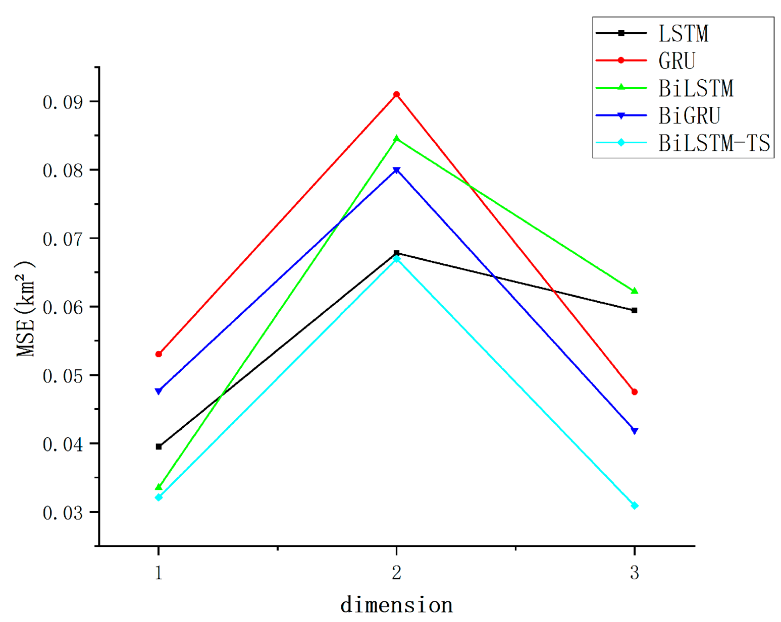
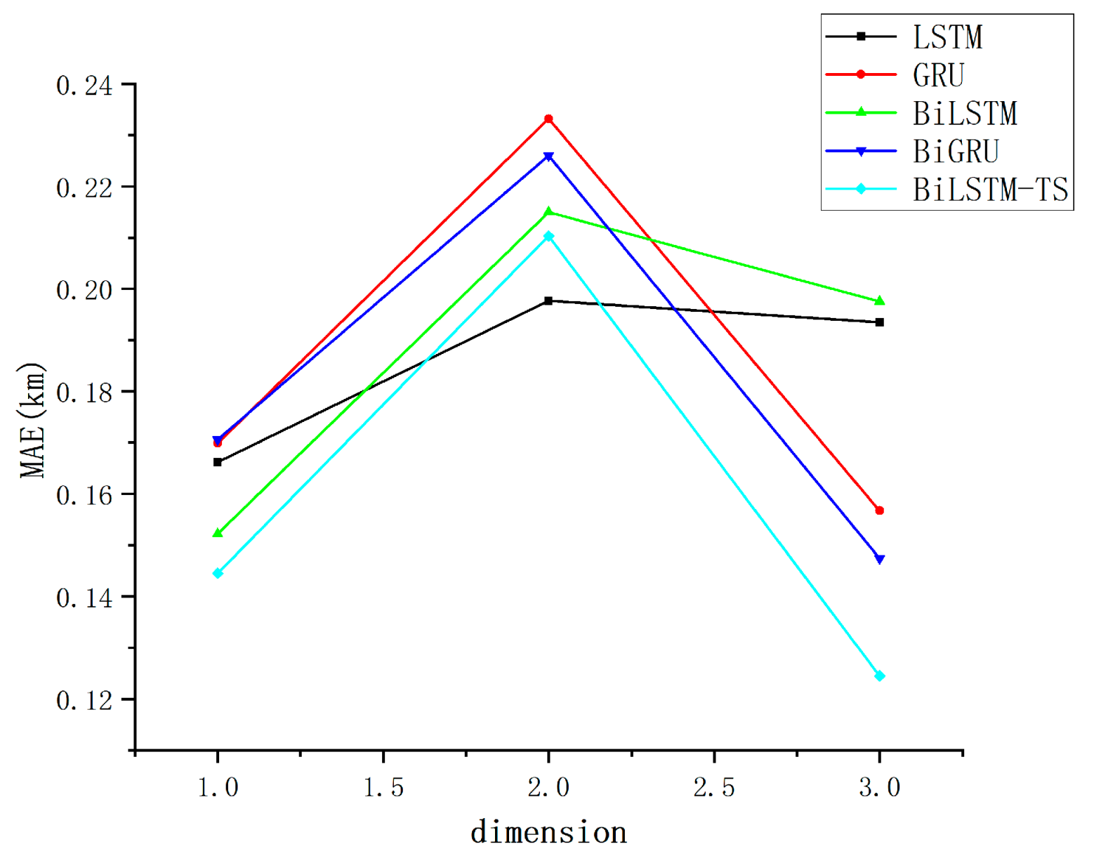
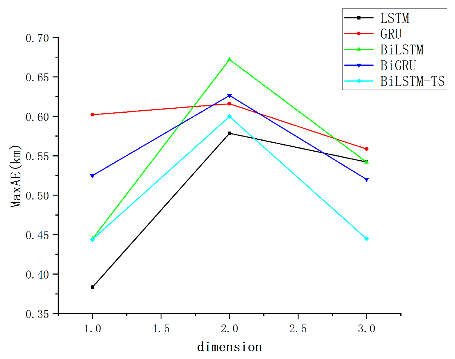
In such scenarios, the complexity of these models often becomes a liability, resulting in subpar performance. Studying lightweight models has the potential to improve model performance and increase efficiency [31]. Removing the Transformer and its variants from the model allows for a better comparison of the effectiveness of the remaining models, as shown in Figure 7, Figure 8 and Figure 9.
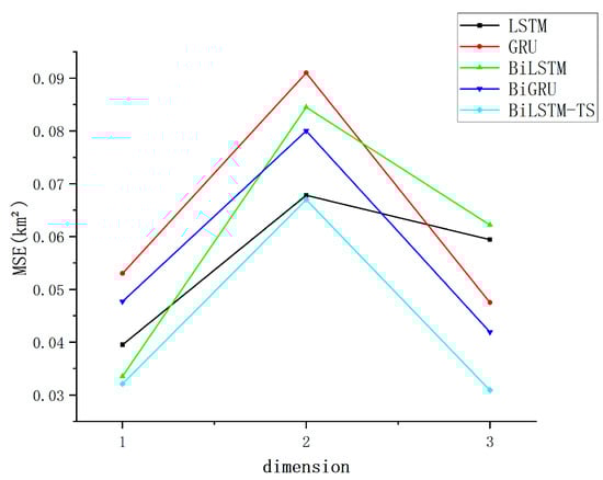
Figure 7.
Multi-model MSE assessment metrics dot plot.
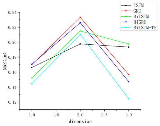
Figure 8.
Multi-model MAE assessment metrics dotted line plot.
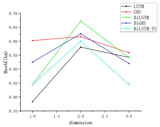
Figure 9.
Multi-model MaxAE assessment indicator dot plot.
The strong performance of the other models with simple feature inputs can primarily be attributed to their exceptional modeling capabilities and flexibility in handling time series data. LSTM and GRU networks leverage their gating mechanisms to effectively capture long-term dependencies, thereby mitigating the issue of vanishing gradients. Meanwhile, bidirectional models, such as BiLSTM and BiGRU, extend this capability by incorporating both past and future temporal information, enabling them to uncover deeper patterns from the global features of the data. The improved BiLSTM-TS model further enhances the representation of time series by integrating additional features captured through trend and season blocks. These models do not require complex feature engineering; even with relatively simple inputs, they are able to selectively memorize and extract critical patterns through their recursive structures and gating mechanisms. This results in a robust adaptability to low-dimensional features, along with an outstanding ability to generalize across diverse datasets. Since the effect gap between different models is small, in order to more intuitively show the forecasting ability of different models, the data are organized and counted, and the track forecasting accuracy indexes are obtained, as presented in Table 2.
Table 2.
MSE, MAE, and MaxAE accuracy metrics for multiple models with different dimensional feature inputs.
Among the evaluated architectures, Transformer-based networks and their derivatives exhibit suboptimal performance in scenarios involving single-feature inputs. However, a marked performance enhancement is observed as the input feature dimensionality increases, underscoring their inherent suitability for complex predictive tasks requiring multivariate data integration.
The diminished efficacy under single-feature constraints likely stems from two interrelated factors: model capacity and data sufficiency and feature expressiveness limitations.
Model capacity and data sufficiency: The high parameterization and representational flexibility of Transformer architectures demand extensive training data to effectively regularize their learning process. When limited to single-feature inputs, the restricted informational complexity of the dataset fails to adequately constrain these high-capacity models, creating a mismatch between model complexity and data richness.
Feature expressiveness limitations: While Transformers excel at capturing nonlinear interdependencies through self-attention mechanisms, their performance is contingent on the input features’ ability to encode sufficient predictive signals. Single-feature inputs inherently lack the complementary information required to disentangle complex temporal patterns, thereby reducing the model’s ability to generalize beyond training distributions.
This phenomenon aligns with established machine learning principles; overparameterized models like Transformers are particularly vulnerable to overfitting in low-data regimes, where the limited feature space cannot provide the necessary discriminative power to guide robust parameter estimation. Empirical observations suggest that while Transformer variants theoretically possess superior pattern recognition capabilities, their practical utility in resource-constrained or feature-sparse environments remains contingent on careful architectural adaptation or data augmentation strategies.
As shown in Table 2, the bolded values indicate the optimal results under identical evaluation conditions. When employing MSE as the evaluation criterion, the BiLSTM-TS model demonstrates stable performance and achieves the best results, while remaining competitive under alternative metrics. Compared to the baseline BiLSTM model, the enhanced BiLSTM-TS architecture—incorporating trend and seasonal blocks—exhibits superior forecasting accuracy. This improvement underscores the critical role of the added modules in capturing both long-term trend patterns and periodic fluctuations embedded within the time series data.
3.2. Prediction Error
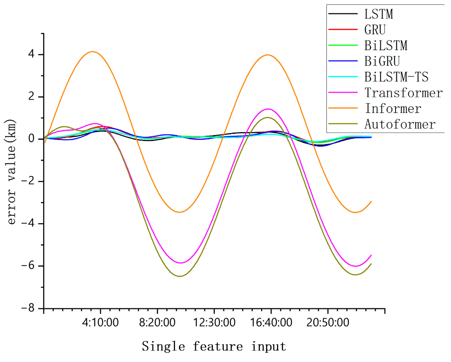
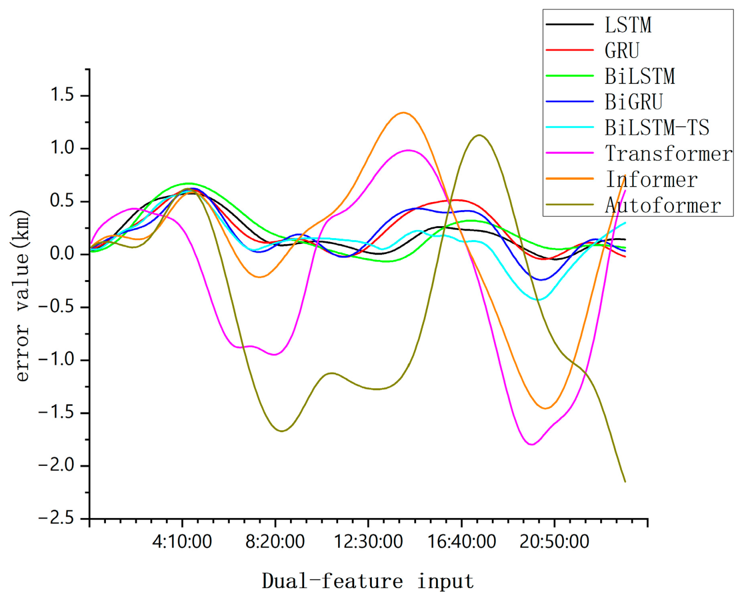
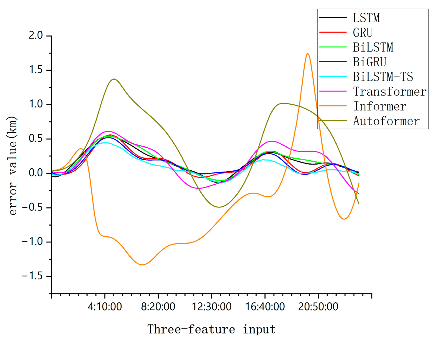
Historical prediction data from 17 December to 26 December 2023 serve as the input, while the predicted data for 27 December 2023 are designated as the output. Given the SP3 precise ephemeris file’s five-minute sampling interval, the ten-day period yields 2881 data points, which are used to forecast 288 future orbital positions. Taking the BeiDou-2 M6 (C14) satellite as an example, its single-day prediction error results are illustrated in Figure 10, Figure 11 and Figure 12:
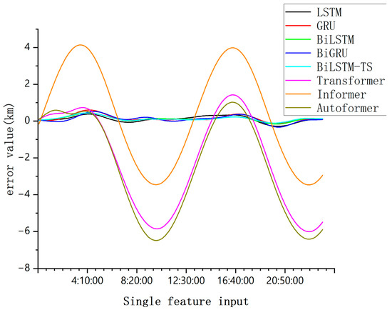
Figure 10.
Comparison of single-day forecast errors of each model with single feature input.
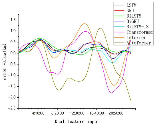
Figure 11.
Comparison of single-day forecast errors of each model under dual-feature input.
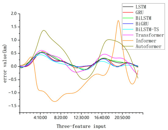
Figure 12.
Comparison of single-day forecast errors of each model when three characteristics are input.
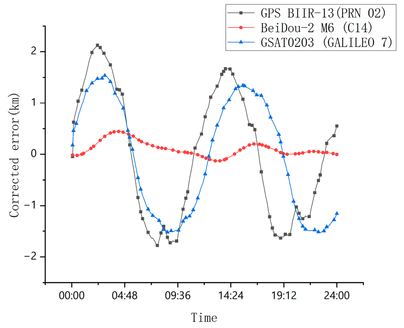
To validate the generalizability of the BiLSTM-TS model across diverse satellite systems, this study selects GPS BIIR-13 (PRN 02), BeiDou-2 M6 (C14), and GSAT0203 (GALILEO 7) as representative satellites for numerical simulations. When three-dimensional features are utilized as inputs, the residual errors for each satellite system are illustrated in Figure 13.
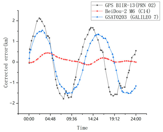
Figure 13.
Represents satellite-corrected error.
From Figure 10, Figure 11, Figure 12 and Figure 13, this comparison highlights a crucial distinction; simpler models tend to converge effectively when handling basic data features, while more complex models have higher data demands and are more prone to overfitting when data are insufficient.
However, the BiLSTM-TS model demonstrates a clear advantage in orbit prediction. When tested on mid-orbit satellite trajectory forecasting, the BiLSTM-TS model significantly outperforms traditional models in terms of accuracy. For example, in the case of the BeiDou-2 M6(C14) satellite, after applying the BiLSTM-TS model, the maximum absolute error in the x-axis position was reduced from 4.0625 km to 0.4448 km. This substantial reduction in prediction error clearly illustrates the effectiveness of the BiLSTM-TS model in improving orbit prediction accuracy.
To further validate the model’s generalizability, we included two additional satellites for testing: GPS BIIR-13 (PRN 02) and GSAT0203 (GALILEO 7). These satellites effectively represent GPS and Galileo systems, showcasing the model’s versatility. Experimental results demonstrate a dramatic improvement in X-axis positioning accuracy; the GPS BIIR-13 (PRN 02) achieved a 96.1% error reduction, decreasing from 54.7681 km to 2.1261 km, while the GSAT0203 (GALILEO 7) exhibited an even more significant 96.8% precision enhancement, plummeting from 47.5542 km to 1.5376 km. These quantitative outcomes underscore the BiLSTM-TS model’s versatile applicability across diverse MEO satellite architectures, spanning distinct navigation systems and orbital regimes.
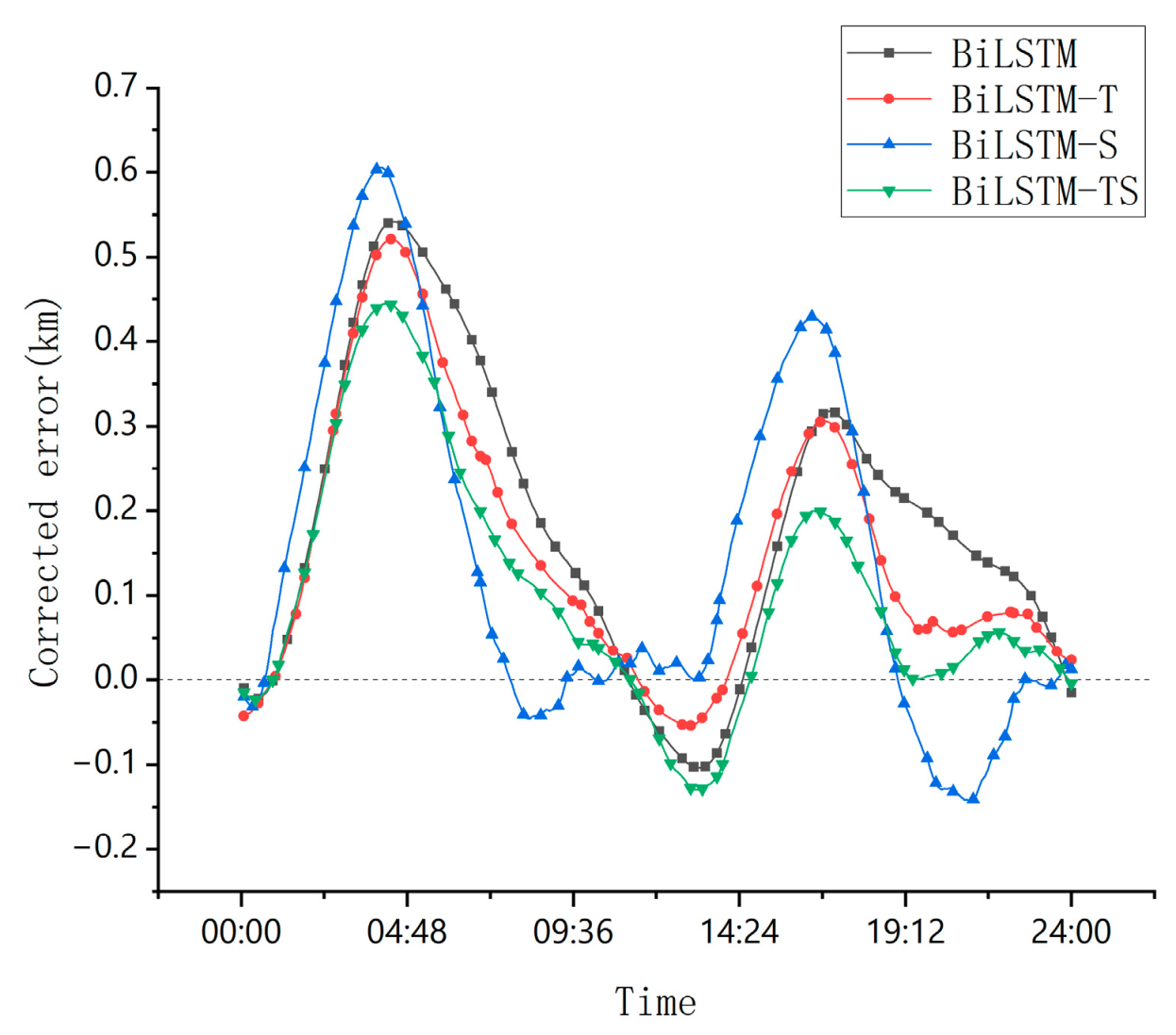
3.3. Ablation Experiment
To systematically evaluate the effectiveness of model components, this study designs a four-tiered ablation study framework (Figure 14), comprising the following comparative models:
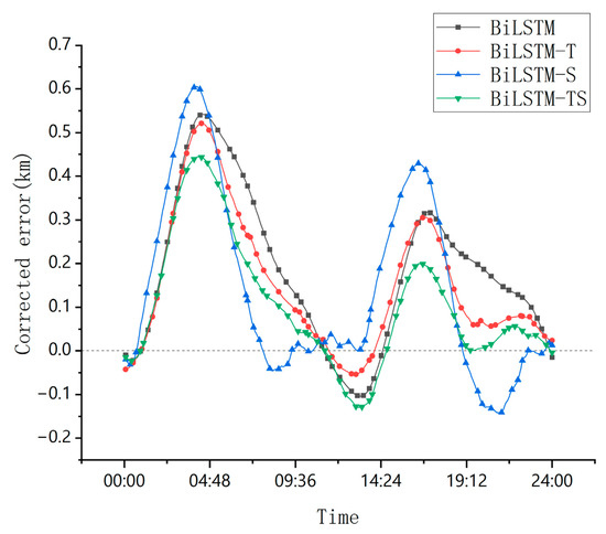
Figure 14.
Ablation experiments with comparison of the corrected errors for each model.
- Baseline Model: BiLSTM;
- Trend-Enhanced Variant: BiLSTM-T (BiLSTM + Trend Module);
- Seasonality-Enhanced Variant: BiLSTM-S (BiLSTM + Season Module);
- Full Model: BiLSTM-TS (BiLSTM + Trend Module + Season Module).
The experiments employ a controlled variable approach for MEO satellite orbit prediction tasks, with fixed hidden layer dimensions and training strategies. This study utilizes 3D position data as an input feature to specifically monitor the corrected error in orbit prediction over a 24 h period.
3.4. Deep Learning Benefits
In order to illuminate the advantages and disadvantages of incorporating deep learning into orbit prediction, this article presents a comparative analysis in terms of computational cost, long-term prediction stability, and confidence intervals.
In the experiments, the computational cost of the prediction model was analyzed in terms of four aspects: task execution time, throughput, average CPU usage, and average memory footprint at the time of prediction. Analyzing the computation cost provides a comprehensive measure of system efficiency, resource utilization, and performance bottlenecks, thus supporting accurate cost control and optimization decisions.
As can be seen from Table 3, the throughput of the SGP4 model is much higher than that of the deep learning model, mainly due to the fact that the SGP4 model adopts an analytical approach for orbit computation, while the deep learning model usually relies on complex numerical computation and large-scale parameter optimization. The SGP4 model generates orbit predictions quickly through analytical formulas, with low computational complexity, which makes it suitable for real-time processing and fast computation of large-scale data. In contrast, deep learning models require a large amount of computational resources and have high computational complexity and resource requirements during inference, which limits their throughput. In addition, the simplified ingestion processing and optimized algorithm design of the SGP4 model further improve its computational efficiency.
Table 3.
Computational costs of different models in predicting orbital data for a future day.
There is little difference in computational cost between different models, in which GRU and BiGRU, as lightweight models, significantly outperform other deep learning models in terms of average CPU utilization.
The task execution time of the deep learning model is several orders of magnitude higher than that of the SGP4 model, but it is still possible to obtain track forecasting results quickly enough to satisfy the usage requirements in terms of time.
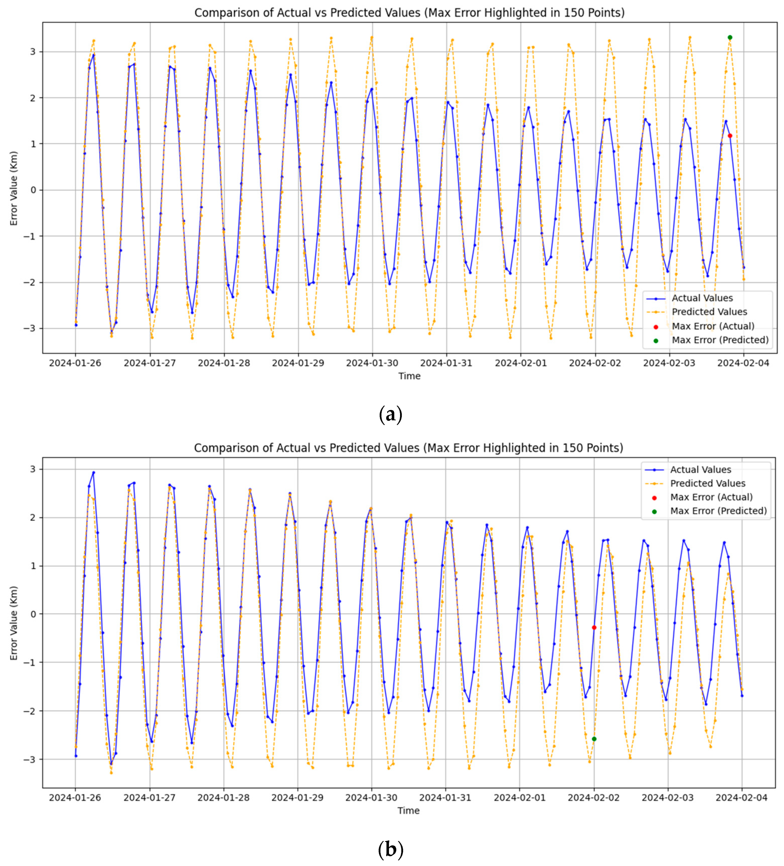
In order to verify the performance of the model in terms of long-term prediction stability under different data, the original data were expanded from one day to forty days (containing 11,521 data) and the prediction time was expanded from one day to nine days (containing 2592 data).
As can be seen in Figure 15, the forecast error increases when the prediction time changes from 1 day to 9 days, and the prediction error for a period of nine days forms a peak near the exact value under the influence of deep learning. This phenomenon implies that deep learning is able to minimize the overall error on the basis of SGP4. In addition, when the amount of historical data is expanded to 40 days, the fluctuation range of the prediction error becomes smaller, and the forecast accuracy is improved.

Figure 15.
(a) SGP4 predicts the day ahead; (b) SGP4 predicts the next nine days; (c) BiLSTM-TS model to predict one day ahead with ten days of historical data; (d) BiLSTM-TS model to predict the next nine days with ten days of historical data; (e) BiLSTM-TS model predicts one day ahead with forty days of historical data; (f) BiLSTM-TS model to predict the next nine days with forty days of historical data.
From Figure 16, it can be seen that when the prediction time is prolonged, the prediction results start to be unstable, which means that the ability of the model to predict in the long term needs to be further improved. The model can be further optimized by adjusting the hyperparameters, choosing a suitable optimization algorithm, and changing the model. This will also be investigated in future research.
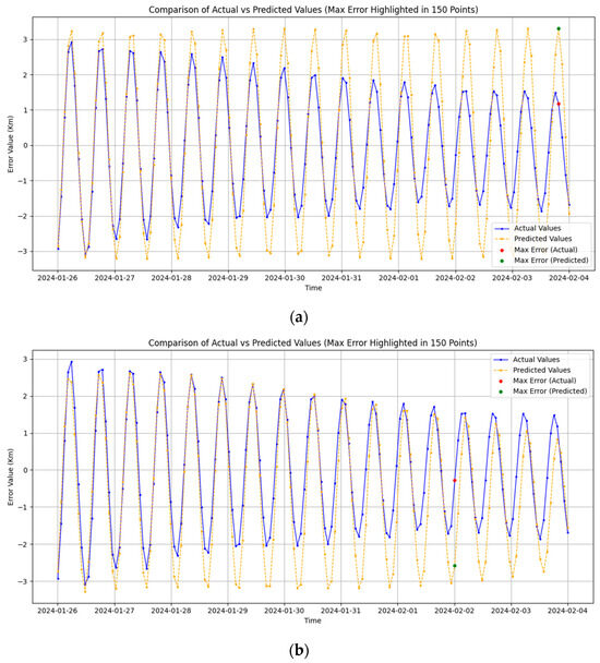
Figure 16.
(a) Comparison of true and predicted values when predicting data for the next nine days with ten days of historical data; (b) comparison of true and predicted values when predicting data for the next nine days with forty days of historical data.
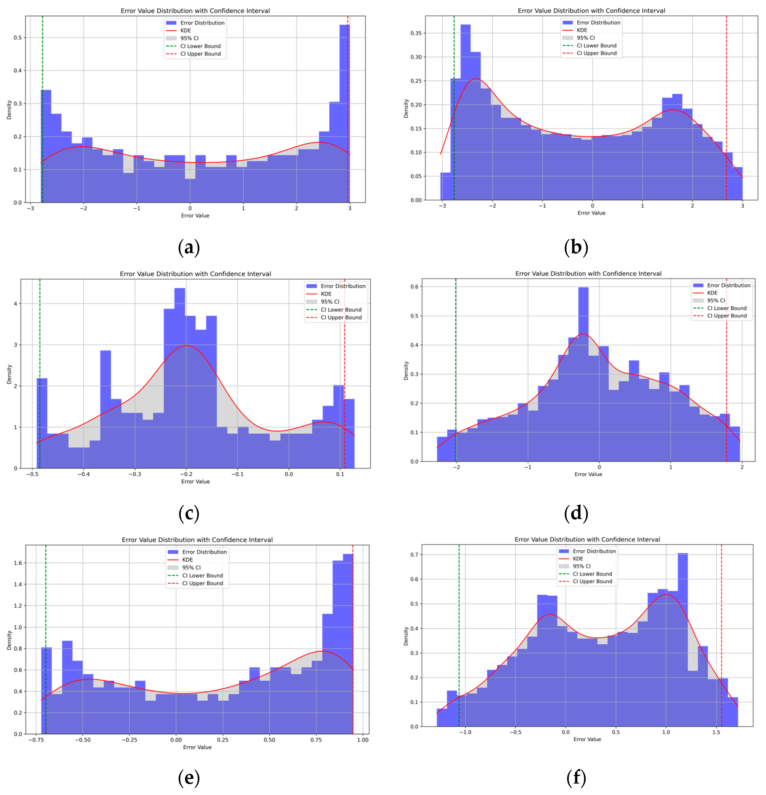
Confidence intervals for the orbital errors under the SGP4 model and under the BiLSTM-TS model were determined by analyzing the data and experiments, and this value was used as a measure of prediction accuracy. At a confidence level of 95%, the confidence interval of the data is recorded, and the narrower the confidence interval and the closer it is to 0, the higher the prediction accuracy. Confidence intervals for the SGP4 versus BiLSTM-TS model are recorded in Table 4.
Table 4.
Confidence intervals for different models under different conditions.
In terms of confidence intervals, the range of confidence intervals under the BiLSTM-TS model is much narrower, and the confidence intervals increase in range as the prediction time increases.
4. Discussion
During the experiment, the performance difference between the SGP4 model and the deep learning model was compared after analyzing the data and visualizing the presentation. In the overall comparison of different models, different data sizes and different prediction lengths, it can be found that the BiLSTM-TS model can effectively reduce the prediction error and improve the prediction accuracy. Changes in data size can significantly affect the prediction results, and when the data size increases, the prediction results are more stable, and the accuracy has a certain decline compared to small samples. When the data volume is larger, the model pays more attention to the long-term trend and easily ignores the detailed changes; when the data volume is smaller, the model becomes less robust.
Additionally, we conducted an ablation study, which is valuable for understanding the contribution of different model components to overall performance. By systematically removing certain components or features from the model, we were able to assess their impact on predictive accuracy. This approach helps identify the key components and functions that drive model performance. Our findings indicate that simply adding a seasonal block to the BiLSTM-TS model did not result in a significant performance improvement. However, incorporating only the trend block led to a small performance gain. The most substantial improvement was observed when both the seasonal and trend blocks were included, indicating a considerable enhancement in model performance. This demonstrates that the BiLSTM-TS model’s ability to capture both seasonal and trend components plays a crucial role in its outstanding predictive accuracy.
5. Conclusions
Satellite orbit prediction, particularly for MEO satellites, presents significant challenges in space science and engineering due to complex dynamical perturbations. Conventional methods, such as the SGP4 model, rely on simplified physical assumptions and analytical approximations, which lead to substantial deviations when addressing nonlinear orbital variations, external perturbations (such as atmospheric drag and third-body gravitational effects), and long-term predictions beyond seven days. While these models perform adequately for short-term predictions (less than 24 h), their limitations in accuracy have driven the need for advanced deep learning techniques in orbit determination.
The proposed BiLSTM-TS model leverages the strengths of BiLSTM networks in modeling temporal sequences. Unlike unidirectional LSTMs, the BiLSTM architecture captures both forward (past-to-future) and backward (future-to-past) temporal dependencies, enhancing the model’s ability to predict short-term fluctuations, long-term trends, and nonlinear transitions. The model is designed to handle high-frequency orbital perturbations, secular orbital drifts due to lunisolar resonances, and state discontinuities that occur during station-keeping maneuvers. This bidirectional approach significantly improves prediction stability.
Experimental validation of the BiLSTM-TS model shows substantial improvements in addressing three core challenges in orbit prediction: nonlinear dynamics, perturbation sensitivity, and long-term error accumulation. The performance of the BiLSTM-TS model in daily prediction tasks shows significant accuracy, with a 94.2% improvement in Mean Squared Error (0.0309 km2), a 91.8% reduction in Mean Absolute Error (0.1245 km), and an 88.9% decrease in Maximum Position Error (0.4448 km).
In order to further improve the model performance, this paper verifies the superiority of BiLSTM-TS in orbit prediction by comparing and analyzing the performance of different models with multiple feature inputs. By increasing the dimensionality of input features, the performance of Transformer and its variant models is also improved, and this result provides a valuable reference for future research on deep learning-based satellite orbit prediction. Next, a more in-depth study will be conducted from the perspective of the dimensionality of the data features and the complexity of the data itself to explore the impact of the data on the model performance and to find the most suitable feature combination and model architecture.
In addition, the study in this paper was conducted within the framework of the traditional SGP4 track forecasting model and by analyzing the prediction errors of the TLE data, and did not involve traditional model optimization or feature input optimization. Future research will further consider these two directions with a view to further improving the accuracy of track prediction without sacrificing computational efficiency. The in-depth discussion of the factors affecting the accuracy of path prediction will provide new ideas and methods for realizing high-precision satellite orbit prediction.
Author Contributions
Conceptualization, Y.G.; methodology, B.L.; software, Z.Z. and B.L.; validation, Y.G., B.L. and J.W.; formal analysis, J.S. and B.L.; resources, Y.G. and J.S.; data curation, X.S. and B.L.; writing—original draft preparation, B.L.; writing—review and editing, Y.G. and B.L.; funding acquisition, X.S., Y.G. and Z.Z. All authors have read and agreed to the published version of the manuscript.
Funding
This research was funded by the Open Fund Project of Key Laboratory of Intelligent Space TTC&O (Space Engineering University), Ministry of Education, NO. CYK2024-02-06 and Shandong Key Laboratory of Space Debris Monitoring and Low-orbit Satellite Networking, NO. CK-2024-0050.
Data Availability Statement
The original contributions presented in this study are included in this article. Further inquiries can be directed to the corresponding author.
Conflicts of Interest
Author Jinsheng Wang was employed by the company Universe Kingdom Beijing Technology Co., Ltd. The remaining authors declare that the research was conducted in the absence of any commercial or financial relationships that could be construed as a potential conflict of interest.
Abbreviations
The following abbreviations are used in this manuscript:
| BiGRU | Bidirectional Gated Recurrent Unit |
| BiLSTM | Bidirectional Long Short-Term Memory |
| BiLSTM-TS | Bidirectional Long Short-Term Memory with Trend and Season |
| ECEF | Earth-Centered, Earth-Fixed |
| GNSS | Global Navigation Satellite Systems |
| GPS | Global Positioning System |
| GRU | Gated Recurrent Unit |
| LSTM | Long Short-Term Memory |
| MAE | Mean Absolute Error |
| MaxAE | Maximum Absolute Error |
| MEO | Medium-Earth Orbit |
| MSE | Mean Square Error |
| NORAD | North American Aerospace Defense Command |
| SGP4 | Simplified General Perturbations Model 4 |
| SP3 | Standard Product 3 |
| TEME | True Equator, Mean Equinox |
| TLE | Two-Line Element set |
References
- Yang, C.; Zang, B.; Gu, B.; Zhang, L.; Dai, C.; Long, L.; Zhang, Z.; Ding, L.; Ji, H. Doppler Positioning of Dynamic Targets with Unknown LEO Satellite Signals. Electronics 2023, 12, 2392. [Google Scholar] [CrossRef]
- Xiao, Y.; Guo, Y.; Pang, Q.; Yang, X.; Zhao, Z.; Yin, X. STar-DETR: A Lightweight Real-Time Detection Transformer for Space Targets in Optical Sensor Systems. Sensors 2025, 25, 1146. [Google Scholar] [CrossRef]
- Guo, Z.; Yin, X.; Zhao, Z.; Yang, X. Near-Earth space target tracking based on Unscented Kalman Filter. In Proceedings of the 2024 4th International Conference on Electronic Information Engineering and Computer (EIECT), Shenzhen, China, 15–17 November 2024; pp. 750–754. [Google Scholar] [CrossRef]
- Guo, Y.; Yin, X.; Xiao, Y.; Zhao, Z.; Yang, X.; Dai, C. Enhanced YOLOv8-based method for space debris detection using cross-scale feature fusion. Discov. Appl. Sci. 2025, 7, 95. [Google Scholar] [CrossRef]
- Cheng, Z.; Guo, Y.; Zhao, Z.; Zhang, Q.; Yu, C. Experimental design of the twin control system for space object monitoring equipment. Mod. Manuf. Technol. Equip. 2023, 59, 126–129. [Google Scholar] [CrossRef]
- Guo, Y.; Cheng, Z.; Zhang, Q.; Zhao, Z. Performance evaluation method of the space object collaborative monitoring system based on fuzzy theory. Mod. Radar 2024, 46, 127–135. Available online: https://link.cnki.net/urlid/32.1353.TN.20231107.0948.002 (accessed on 21 April 2025).
- Chen, X.; Dai, W.; Zhang, M.; Bian, L.; Tang, C.; Li, K. Prediction of atmospheric drag coefficient based on Bi-LSTM neural network. Geod. Geodyn. 2024, 44, 1161–1166. [Google Scholar] [CrossRef]
- Liu, H.; Xia, S.; Sang, J. Application of random forest in determining the drag coefficient of low Earth orbit space targets. Surv. Mapp. Geogr. Inf. 2024, 49, 33–37. [Google Scholar] [CrossRef]
- Li, X.; Li, J.; Yuan, Y.; Zheng, H.; Huang, S.; Liu, C.; Zhang, K. Analysis and refinement of the empirical solar radiation pressure model for BeiDou-3 satellites. J. Surv. Mapp. 2022, 51, 1680–1689. [Google Scholar]
- Zhu, H.; Liu, S.; Li, C.; Tang, L.; Yang, H. GNSS ultra-fast orbit prediction considering solar radiation pressure model and sampling interval. Surv. Sci. 2024, 49, 1–14. [Google Scholar] [CrossRef]
- Zhang, X.; Liu, Y.; Song, J. Short-term orbit prediction based on LSTM neural network. Syst. Eng. Electron. 2022, 44, 939–947. [Google Scholar]
- Han, Y. Study on Orbital Smoothing and Prediction Algorithm for Spacecraft Based on Limited Observation Data. Doctoral Dissertation, Central South University, Changsha, China, 2022. Available online: https://link.cnki.net/doi/10.27661/d.cnki.gzhnu.2022.001742 (accessed on 21 April 2025).
- Sun, Y.; Meng, F.; Wu, N.; Zhao, Y. Performance analysis of ballistic prediction using analytical geometry and numerical integration methods. J. Inf. Eng. Univ. 2016, 17, 635–640. [Google Scholar]
- Li, B.; Sang, J.; Ning, J. Performance analysis of semi-analytical orbital prediction method for space debris. Infrared Laser Eng. 2015, 44, 3310–3316. [Google Scholar]
- Han, Y. Research on orbital prediction algorithm based on LSTM neural network. Sci. Technol. Innov. 2022, 21, 88–91. [Google Scholar]
- Ji, X.; Lu, C.; Xie, B.; Guo, H.; Zheng, B. Combination of a Rabbit Optimization Algorithm and a Deep-Learning-Based Convolutional Neural Network–Long Short-Term Memory–Attention Model for Arc Sag Prediction of Transmission Lines. Electronics 2024, 13, 4593. [Google Scholar] [CrossRef]
- Guo, Y.; Li, B.; Pang, Q.; Yang, X.; Zhao, Z.; Liu, X. LSTM-BP model: Enhancing prediction accuracy for Medium Earth Orbit satellites. In Proceedings of the 2024 4th International Conference on Electronic Information Engineering and Computer (EIECT), Shenzhen, China, 15–17 November 2024; pp. 703–706. [Google Scholar] [CrossRef]
- Cao, C.; Huang, J.; Wu, M.; Lin, Z.; Sun, Y. A Multivariate Time Series Prediction Method Based on Convolution-Residual Gated Recurrent Neural Network and Double-Layer Attention. Electronics 2024, 13, 2834. [Google Scholar] [CrossRef]
- Yang, M.; Chen, Y.; Fang, G.; Ma, C.; Liu, Y.; Wang, J. A Short-Term Power Load Forecasting Method Based on SBOA–SVMD-TCN–BiLSTM. Electronics 2024, 13, 3441. [Google Scholar] [CrossRef]
- Zhong, Y.; He, T.; Mao, Z. Enhanced Solar Power Prediction Using Attention-Based DiPLS-BiLSTM Model. Electronics 2024, 13, 4813. [Google Scholar] [CrossRef]
- Zhou, R.; Qiu, S.; Li, M.; Meng, S.; Zhang, Q. Short-Term Air Traffic Flow Prediction Based on CEEMD-LSTM of Bayesian Optimization and Differential Processing. Electronics 2024, 13, 1896. [Google Scholar] [CrossRef]
- Liu, S.; Qiu, S.; Li, H.; Liu, M. Real-Time Telemetry-Based Recognition and Prediction of Satellite State Using TS-GCN Network. Electronics 2023, 12, 4824. [Google Scholar] [CrossRef]
- Yang, K.; Wang, Y.; Han, X.; Cheng, Y.; Guo, L.; Gong, J. Unsupervised Anomaly Detection for Time Series Data of Spacecraft Using Multi-Task Learning. Appl. Sci. 2022, 12, 6296. [Google Scholar] [CrossRef]
- Chen, H.; Liu, S.; Yang, X.; Zhang, X.; Yang, J.; Fan, S. Prediction of Sunspot Number with Hybrid Model Based on 1D-CNN, BiLSTM and Multi-Head Attention Mechanism. Electronics 2024, 13, 2804. [Google Scholar] [CrossRef]
- Guo, D.; Meng, L.; Yu, L.; Shi, W.; Li, S.; Fan, L.; Yu, J.; Jiang, Y. Research and application of high-resolution multi-mode satellite space-ground integrated engineering. Spacecr. Eng. 2022, 31, 24–30. [Google Scholar]
- Chen, S.; Du, L. Autonomous orbit determination of Quasi-Relay Satellite and BeiDou Navigation Satellites in single-link mode. J. Surv. Sci. Technol. 2020, 37, 362–367. [Google Scholar]
- Liu, J.; Wu, C.; Xu, J.; Du, J.; Lei, X. Space event and outlier detection based on expectation maximization algorithm. J. Space Sci. 2022, 42, 1185–1192. [Google Scholar] [CrossRef]
- Thammawichai, M.; Luangwilai, T. Data-driven satellite orbit prediction using two-line elements. Astron. Comput. 2024, 46, 100782. [Google Scholar] [CrossRef]
- Ding, S.; He, D.; Liu, G. Improving Short-Term Load Forecasting with Multi-Scale Convolutional Neural Networks and Transformer-Based Multi-Head Attention Mechanisms. Electronics 2024, 13, 5023. [Google Scholar] [CrossRef]
- Jiao, L.; Wang, M.; Liu, X.; Li, L.; Liu, F.; Feng, Z.; Yang, S.; Hou, B. Multiscale deep learning for detection and recognition: A comprehensive survey. IEEE Trans. Neural Netw. Learn. Syst. 2025, 36, 5900–5920. [Google Scholar] [CrossRef]
- Jeong, S.; Shin, Y. LTE: Lightweight Transformer Encoder for Orbit Prediction. Electronics 2024, 13, 4371. [Google Scholar] [CrossRef]


Disclaimer/Publisher’s Note: The statements, opinions and data contained in all publications are solely those of the individual author(s) and contributor(s) and not of MDPI and/or the editor(s). MDPI and/or the editor(s) disclaim responsibility for any injury to people or property resulting from any ideas, methods, instructions or products referred to in the content. |
© 2025 by the authors. Licensee MDPI, Basel, Switzerland. This article is an open access article distributed under the terms and conditions of the Creative Commons Attribution (CC BY) license (https://creativecommons.org/licenses/by/4.0/).