Abstract
With the rapid development of deep learning, weather recognition has become a research hotspot in the field of computer vision, and the research on field programmable gate array (FPGA) acceleration based on deep learning algorithms has received more and more attention, based on which, we propose a method to implement deep neural networks for weather recognition in a small-scale FPGA. First, we train a deep separable convolutional neural network model for weather recognition to reduce the parameters and speed up the performance of hardware implementation. However, large-scale computation also brings the problem of excessive power consumption, which greatly limits the deployment of high-performance network models on mobile platforms. Therefore, we use a lightweight convolutional neural network approach to reduce the scale of computation, and the main idea of lightweight is to use fewer bits to store the weights. In addition, a hardware implementation of this model is proposed to speed up the operation and save on-chip resource consumption. Finally, the network model is deployed on a Xilinx ZYNQ xc7z020 FPGA to verify the accuracy of the recognition results, and the accelerated solution succeeds in achieving excellent performance with a speed of 108 FPS and 3.256 W of power consumption. The purpose of this design is to be able to accurately recognize the weather and deliver current environmental weather information to UAV (unmanned aerial vehicle) pilots and other staff who need to consider the weather, so that they can accurately grasp the current environmental weather conditions at any time. When the weather conditions change, the information can be obtained in a timely and effective manner to make the correct judgment, to ensure the flight of the UAV, and to avoid the equipment being affected by the weather leading to equipment damage and failure of the flight mission. With the help of this design, the UAV flight mission can be better completed.
1. Introduction
Weather recognition is one of the most important research subjects in computer vision. It has a wide range of application scenarios in real life, such as environmental monitoring and quality evaluation [1], agricultural planning [2], outdoor visual system monitoring [3], and weather forecasting [4,5]. It also has important research significance for the smart grid to reasonably dispatch power, develop outdoor robots [6], and for scene understanding. Weather is an important indicator of people’s lives, as different weather has an important impact on people’s clothing, food, housing, and transportation; the most important thing is that with the development of science and technology, in many aspects, precision instruments are often needed to help us carry out some scientific research, and often, these devices are more sensitive to the weather. The accuracy and normal use of the weather need to be considered, for example, the use of GPS (Global Positioning System) equipment and drones. If bad weather is encountered, the impact of weather on UAVs is very significant. Bad weather conditions, such as rain, snow, haze, etc., will a serious effect on the flight stability and operational safety of UAVs. Rain and snow not only increase the weight of the body but also damage electronic components, while haze reduces visibility and affects visual navigation and obstacle-avoidance functions. In addition, extreme temperatures can affect the battery performance and shorten the flight time. Therefore, drones must carefully assess the weather conditions before flying to ensure safety and successful mission completion. Drones have important uses in contemporary life, such as crop detection, pesticide spraying, medical material transportation, emergency rescue, and scientific research. If the weather-recognition system designed in this study can be used in conjunction with UAV flights, the efficiency of UAV work can be greatly improved.
With the continuous development of deep learning technology, convolutional neural networks are widely used in the field of weather image recognition by researchers due to their excellent target recognition and classification capabilities [4,7,8]. Zhu et al. [7] used transfer learning and two convolutional neural networks, Alexnet and GoogLeNet, to identify clear, rainy, and snowy weather in non-fixed scenarios. Liu et al. [9] used sparsely processed Alexnet and Mask R-CNN networks to identify clear, foggy, and snowy weather in non-stationary scenarios.
The use of convolutional neural networks applied to image recognition has been a more popular direction, but now, some of the commonly used convolutional neural network recognitions still have many places that can be improved, and the main purpose of our current study is also to further optimize the performance of convolutional neural networks to recognize the weather. Although the traditional weather-recognition algorithm based on a convolutional neural network can already achieve good accuracy, there is currently an obvious disadvantage of the amount of computation, which is very huge, and this requires a fixed size of the weather image as the recognition object. It is difficult to apply this to the actual embedded devices. Therefore, it needs to be optimized.
The main algorithmic model-optimization techniques commonly used for the huge computational complexity and a lack of memory resources, often encountered in traditional convolutional neural networks, are data quantization [10], singular value decomposition (SVD) [11], pruning, and Hoffman coding [12]. These methods can reduce the number of operations and memory usage of a moving device by compressing the precoding. In addition, deeply separable convolutional neural networks, such as SqueezeNet [13], MobileNet [14], ShuffleNet [15], and Xception [16], greatly reduce the amount of data processing and storage during convolution by converting normal convolution to deep and point-by-point convolution, while still providing high accuracy. For example, compared with VGG-16 [17], the parameters of MobileNet V1 based on depth-separable convolution are reduced by a factor of 32, and the accuracy is only reduced by 0.9%. Therefore, the depth-separable convolutional neural network has low latency. The comparison shows that by using depth-separable convolution, the number of parameters can be greatly reduced, while ensuring that the accuracy will not be greatly affected.
Another area for improvement is speed. Weather-recognition algorithms have high real-time requirements, and the speed of traditional convolutional neural network recognition does not quite meet the real-time requirements, which makes the acceleration design of convolutional neural networks become the current mainstream research direction; the current mainstream acceleration research program can be divided into two aspects: one is the optimization of the algorithm model, and the other is the acceleration of hardware deployment. Hardware deployment acceleration can achieve accelerated performance to better meet the real-time requirements of the convolutional network to identify the weather.
In terms of hardware deployment, the currently available embedded processors are mainly GPUs [18], FPGAs [19], and ASICs [20], but GPUs have the disadvantages of a large size and high power consumption, which cannot be well applied to small mobile devices and terminals, coupled with the long design cycle of ASICs, which cannot be synchronized with the updating of algorithms iteratively, so FPGAs have become the application of the mobile scenario as the platform of choice for convolutional neural network acceleration.
In response to the above analysis, this paper proposes an effective hardware-implementation scheme for weather recognition. This scheme enables the successful deployment of weather-recognition algorithms in FPGAs with low power consumption and hardware resource overhead. The key contributions of this work are summarized as follows: (1) we trained a weather-recognition algorithm model, named Weather-Net, based on a depthwise separable convolutional neural network. Compared with the traditional CNN model, this model has significantly fewer parameters and has 98.2% recognition accuracy based on the Mul-ti-class Weather dataset. (2) We propose a hardware implementation for Weather-Net. In this scheme, the overall architecture and modules of the Weather-Net have been designed and optimized. As a result, weather recognition has been accelerated in FPGA. (3) We implemented the network model on Xilinx ZYNQ xc7z020 FPGA to evaluate the performance of the proposed hardware-implementation scheme. The experimental results show that after the network is deployed on the FPGA platform, the network recognition accuracy can reach 96.8%, the FPGA acceleration performance can reach 108 FPS, and the power consumption is only 3.256 W. According to the above program to complete the design, this design allows the host computer to be connected through the Gigabit network port on the development board; in terms of the application, the image input of this system is the real-time video stream of the road monitoring. To replenish the morality, the host computer collects the video, preprocesses it, and inputs it into the weather-recognition system and then acquires the weather conditions in real-time and transmits the information to the drone pilot and other personnel who are using the precision equipment to perform the drone tasks, accurately grasping the weather conditions and ensuring that the normal flight of the UAV, as well as the measurement accuracy, is not affected.
2. Background
2.1. Traditional Weather-Recognition Method
Traditional weather-classification and recognition methods generally use multi-sensors to obtain weather data, and then, through the mathematical, physical, meteorological, and other knowledge of the data for statistical analysis, this method not only requires sufficient funds and manpower to complete but also a long observation period, with low precision and a large sample size, and it is difficult to apply to intelligent transportation, which requires the large-scale deployment of application scenarios [21].
With the development of intelligent transportation systems and the installation of various monitoring devices on roads, weather images are acquired with the advantages of low cost and efficient acquisition, and weather-image-recognition methods based on image processing and machine vision are beginning to emerge [22,23,24]. This method is generally divided into the following steps: (1) extract feature regions in the image, such as the sky or road area; (2) the specific region to take feature extraction methods to extract weather features, such as spatial pyramid matching and the color histogram method; (3) using machine learning methods to construct classifiers. But this method is more complex in feature extraction and has a lower recognition accuracy, only 50% to 80% accuracy, and cannot accurately determine the weather conditions.
2.2. Weather Recognition Based on Deep Learning
With the rapid growth in the field of deep learning, convolutional neural networks have shown excellent performance in a variety of machine vision tasks [7,8]. Convolutional neural networks can extract abstract, rich, and deep weather features from weather images for end-to-end weather-phenomenon recognition. In many ways, they are superior to weather-recognition methods that rely on sensors and machine learning.
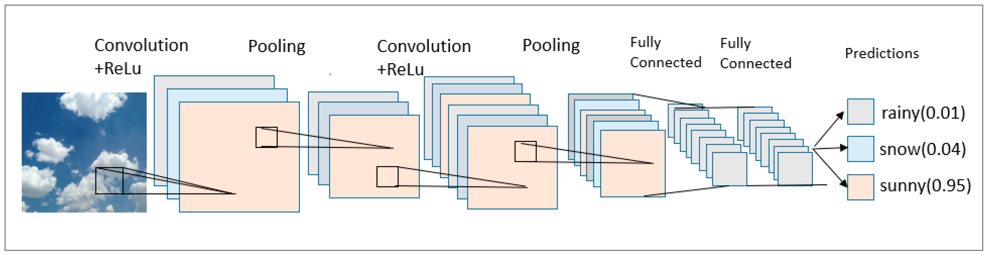
The structural model of a convolutional neural network is similar to that of a Multi-Layer Perceptron (MLP). The main process of CNN is shown in Figure 1.

Figure 1.
A CNN model for weather recognition.
From the above figure, we can clearly see the internal structure in the convolutional neural network model, and you can roughly see the workflow and how to complete the picture recognition.
Although convolutional neural networks are currently effective in the field of image recognition, the parameters and computational effort of their network models are too large for them to be deployed on embedded devices. It is necessary to further improve and optimize the algorithm model.
2.3. Depthwise Separable Convolution Neural Network
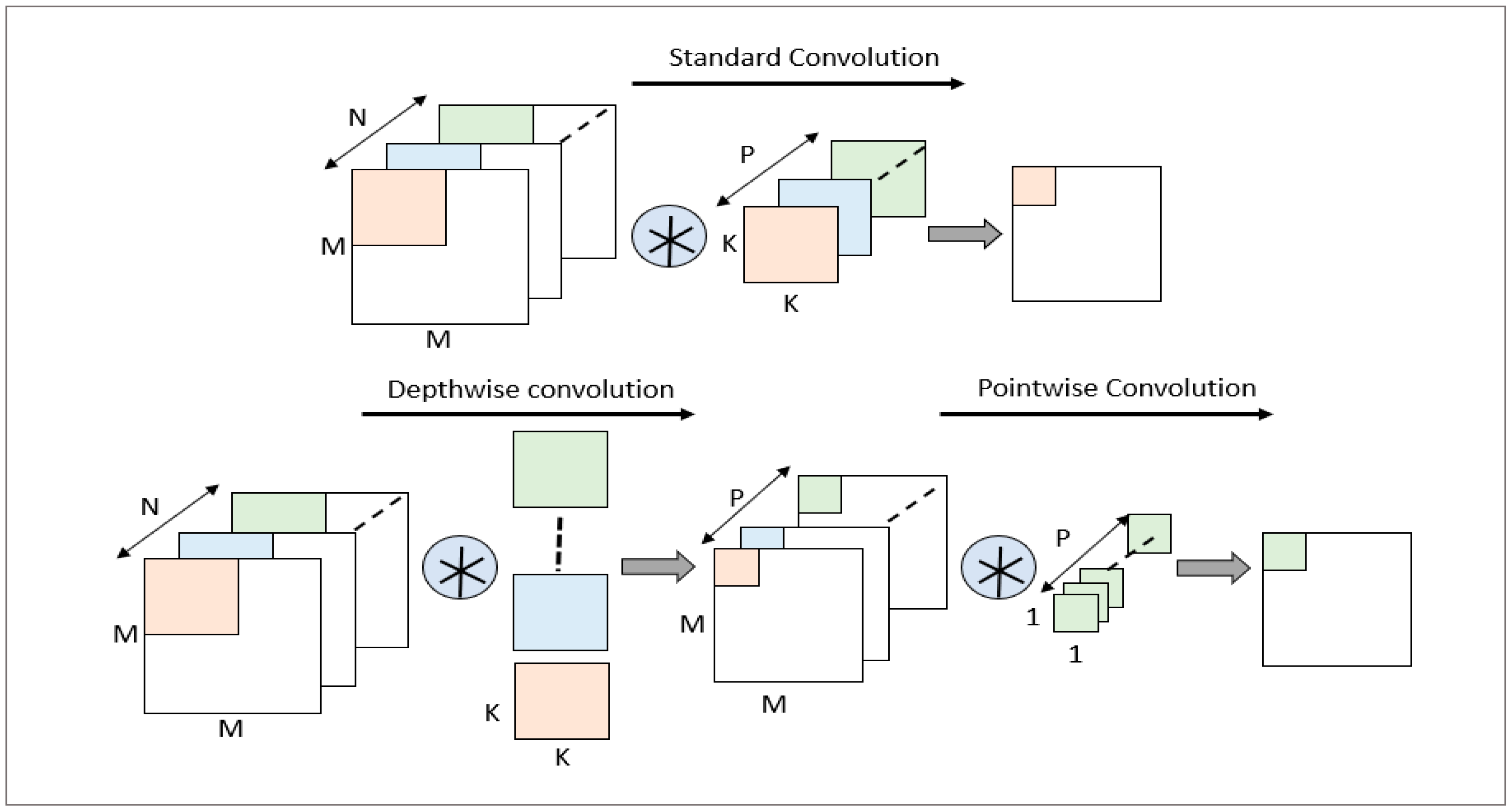
Depthwise Separable Convolution was first proposed by Laurent Sifre [25] in his doctoral dissertation. It decomposes ordinary standard convolution (SC) into two processes: depthwise convolution (DWC) and pointwise convolution (PWC) [16]. In the traditional convolution process, the input feature map is convolved with specific filters (kernels) one by one, and then, the convolution results of each channel are merged to produce the final feature map. When using depthwise separable convolution technology, the system first performs channel-by-channel convolution, that is, it applies convolution operations to each input channel separately. Next, a point-by-point convolution step is performed, which actually uses a conventional 1 × 1 convolution operation. Compared to traditional convolution methods, depthwise separable convolution significantly reduces the complexity of computational operations and can also greatly reduce the computational complexity. Therefore, this is the focus of this article, which uses depthwise separable convolution to optimize algorithms.
Depthwise separable convolution is an efficient convolution operation in convolutional neural networks that decomposes a standard convolutional layer into two independent parts. As shown in Figure 2, the problem with this operation is that it reduces the connection between various data channels but significantly reduces the convolution computation and parameter count.
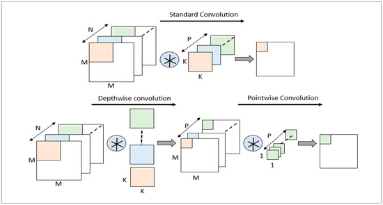
Figure 2.
Comparison of different convolution types.
In order to compensate for the insufficient connection between different channels in channel-by-channel convolution, a point-by-point convolution operation should be performed after running channel-by-channel convolution. Point-wise convolution can weigh and combine the feature maps outputted by channel-wise convolution on different channels, improving the feature correlation between channels.
Assuming the size of the input feature map is A × B × M, and in standard convolution, the size of the convolution kernel is K × K × M, there are a total of N such kernels. Therefore, the total number of convolution kernel weight parameters, WSTC, related to standard convolution is shown in equation as follows:
The total number of operations, TSTC, in standard convolution is shown in the equation, where H and W are the height and width of the output feature map, respectively.
The total number of weight parameters, WDSC, related to depthwise separable convolution is as follows:
The total number of operations in depthwise separable convolution can be given by the following equation:
The ratio of the number of parameters for depthwise separable convolution to standard convolution can be expressed as follows:
The ratio of the total number of operations is
In the above formula, N is the number of channels in the output feature map, and K is the size of the convolution kernel. In practice, the magnitude of N is usually 102, far greater than the value of K, and 1/N can be ignored compared to 1/K2. Therefore, for convolution kernels with a size of 3 × 3, the number of parameters and the total number of operations for depthwise separable convolution operations is about 1/9 of standard convolution, greatly reducing the computational complexity of the network.
2.4. FPGA Hardware Platform
The basic structure of FPGA includes a programmable logic unit, storage unit, routing unit, and I/O pin resources. A programmable logic unit consists of a lookup table (LUT) and a D flip-flop to provide combinational and temporal logic. Storage units include on-chip caching (such as BRAM and LUT) and off-chip storage (such as DDR, SD cards, and Flash). Routing resources connect to logical units inside the FPGA, while I/O pins are used for external communication. The key to deploying a convolutional neural network based on FPGA is that its logical resources can map convolution operations, which can be realized by DSP resources and BRAM on FPGA.
In summary, the key to deploying convolutional neural networks on FPGA is that FPGA has logical resources that can map convolutional neural network functions. Convolutional operations are the core function of convolutional neural networks, which can be deployed to DSP resources on FPGA. The necessary cache resources in the convolution calculation can be implemented by BRAM.
3. Implementation of Weather-Recognition Algorithm
3.1. Selection of Weather Model Recognition Algorithm
The theoretical system of convolutional neural networks has been continuously improved and expanded, so many classic models have appeared. It is because of the proposal and improvement of these models that people have made breakthroughs in the field of image recognition. Among them, the outstanding network models are AlexNet, VGGNet, GoogLeNet, ResNet, and MobileNet.
In this paper, FPGA is chosen as the deployment platform for the inference phase of the weather-recognition algorithm. Therefore, when designing the network model structure, we should not only consider the accuracy of model recognition but also minimize the number of parameters and calculation amount, so as to meet the actual project requirements of deploying the algorithm on FPGA with low power consumption and low resource occupation. Compared with other classical CNN models, the lightweight network MobileNet can greatly reduce the number of model parameters and the amount of computation by using deep separable convolution operations, and it has excellent recognition performance. MobileNet V1 is a lightweight convolutional neural network proposed by Google in 2017, designed for mobile and embedded devices. Its core idea is to drastically reduce the amount of computation and the number of parameters through depthwise separable convolution (DSC), while maintaining better model performance. For example, compared to the VGG16 network with a standard convolutional structure, the accuracy of MobileNet V1 decreased by only 0.9%, while the number of parameters decreased by 90%.
Considering the above situation, this chapter chooses the MobileNet V1 network structure as the initial model and sets the appropriate width factor α and resolution factor β to reduce the network scale, the number of network parameters and the amount of computation. At the same time, in order to facilitate the implementation of FPGA deployment, the relatively simple ReLU activation function can also effectively solve the problem of gradient disappearance in the process of network training.
A few of the parameters mentioned above are briefly described below. α is the width multiplier, which further compresses the model by scaling the number of channels per layer with the parameter α. Its default value is 1.0, which can usually be modified to 0.75, 0.5, and 0.25; when α = 0.5, the number of channels in all layers is halved, and the computation amount is about the original α × α, which is reduced to 25%. β is the resolution multiplier, which typically takes the values of 224, 192, 160, and 128, and the initial value is usually 224. Its function is to reduce the resolution of the input image through the coefficient β and to reduce the computation amount. The input resolution is equal to the multiplication of β with the original resolution. ReLU is the activation function, which typically takes values from 0 to 6 and serves to limit the range of values and enhance the robustness of low-precision computation.
In order to compress the model size to the greatest extent, the width factor α is set to 0.25, and the resolution factor β is set to 0.57; that is, the input feature map size of the network is 128 × 128. Compared with the standard structure MobileNet V1 network, the number of input and output channels of the compressed model is reduced by 4 times, and the size of the input feature image of each layer is correspondingly smaller, which reduces the model scale to a certain extent.
After the compression of the model, the total number of layers remains unchanged, the resolution of the input image of each layer is reduced to 0.57 times, and the number of output channels of each layer is reduced by 4 times. The total number of parameters of the network model before and after compression is shown in Table 1. Compared with the total number of parameters of the standard MobileNet V1 network, the total number of parameters of the model after compression is reduced by 20 times. Specific detailed data comparisons can be visualized in Table 1.

Table 1.
Parameter comparison table before and after compression.
From the comparison of the total number of parameters before and after in Table 1 above, it can be concluded that the compression model can serve to greatly reduce the total number of parameters.
3.2. Weather-Net Network Model Training
3.2.1. Experimental Environment
The experimental environment of this paper is a Windows system, the CPU model is Intel i5-3230M, the memory size is 8 GB, the GPU model is GTX 1650, the video memory size is 4G, and the framework is TensorFlow2.0, CUDA10.0.
3.2.2. Dataset Selection
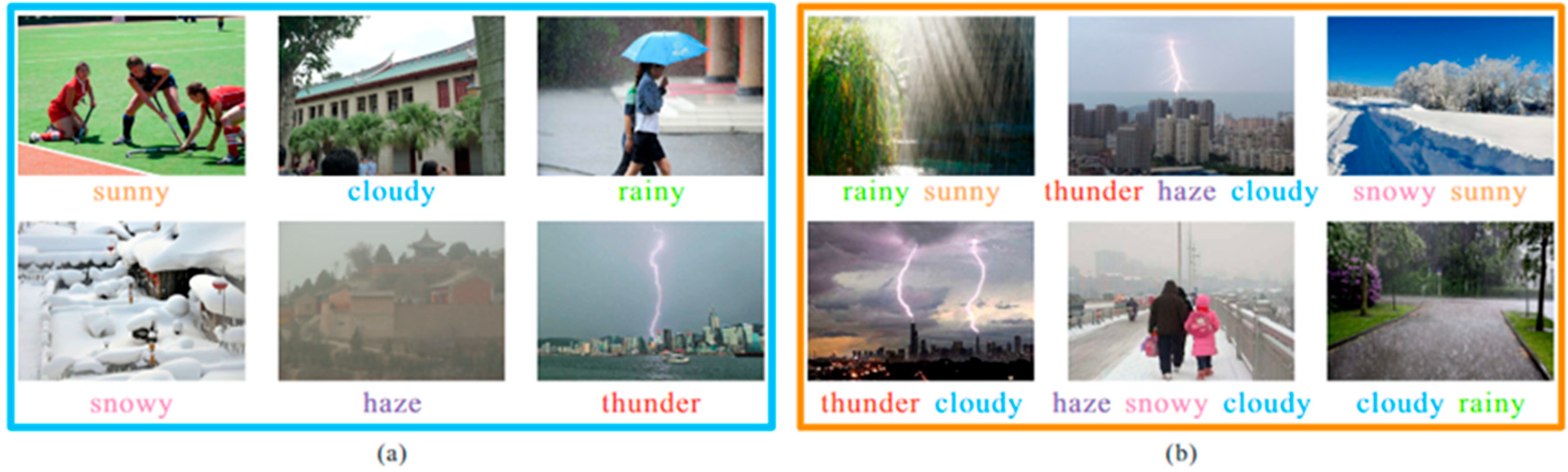
The dataset for training the Weather-Net network model refers to the Multi-class Weather Dataset (MWD) of the Visual Computing Center of Shenzhen University [26]. This dataset contains 65,000 images of six common weather categories: sunny, cloudy, rainy, snowy, haze, and thunderstorm days. Among them, there are 10,000 images for each single weather condition, as shown in Figure 3.

Figure 3.
(a) Simple weather conditions (b) Complex weather conditions.
Since the image size in the MWD dataset is not fixed (ranging from 431 × 400 to 400 × 2029), in order to be consistent with the input layer size in the MobileNet V1 network, it is necessary to preprocess the image in the dataset by using the OpenCV scaling function. All images are scaled to 224 × 224 and 128 × 128, corresponding to the standard MobileNet V1 model structure and the compressed model used in this article, respectively. After that, the rename function is used to rename the image to “weather category_serial number”, the format is uniformly set to JPG, and the image of the same category is saved in the same folder for an easy call during training.
The single weather attribute picture in the total dataset is divided according to the ratio of 8:2, which is respectively used as the model training set and the test set, as shown in Table 2.
Table 2.
Six kinds of weather datasets are composed.
3.2.3. Weather-Net Network Training Scheme
The training set contains 8000 pictures of each type of a single weather attribute and 4000 pictures of multiple weather attributes, and the test dataset contains 2000 pictures of each type of single weather attribute and 1000 pictures of multiple weather attributes.
After building the network model, a more important step is to initialize the weights in the network model. Choosing the appropriate initialization of the weights can avoid the appearance of the gradient disappearance or gradient explosion and accelerate the convergence of the model. In this paper, we use the normal distribution random initialization to set the parameter initialization, the parameters are generated based on a normal distribution with 0 mean and 0.1 variance, and the initial value of the bias parameter is set to 0.
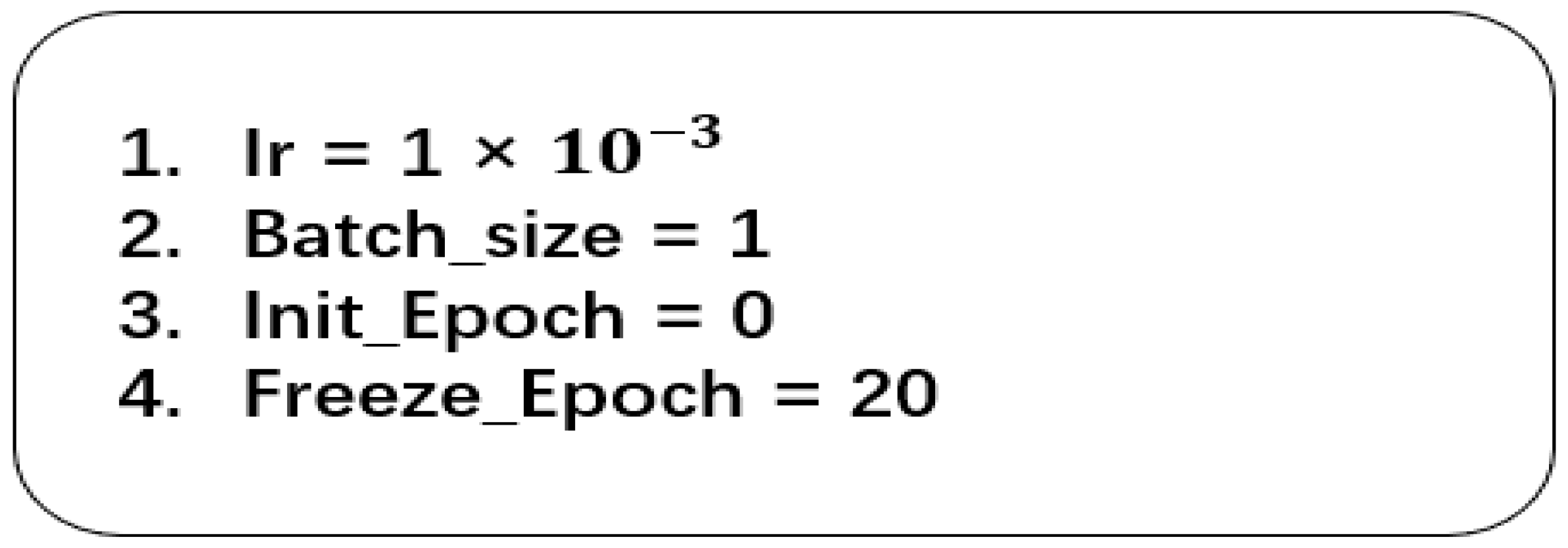
In addition, in deep learning, some parameters cannot be obtained from the learning data and usually need to be set before training, which are called hyperparameters, including the learning rate, batch size, and the number of iterations (epoch). Hyper-parameters are set before the training starts, and usually, the hyper-parameters need to be optimized to give the model a set of optimal hyper-parameters in order to improve the performance and efficiency of learning. Figure 4 below shows the settings of some hyperparameters.

Figure 4.
Setting of hyperparameters.
The first line indicates the setting of the learning rate, which is an important parameter in the training process of neural networks and is often applied to the updating of parameters. It determines how much the model weight parameters are adjusted at each iteration in order to effectively reduce the value of the loss function. The choice of the learning rate can have a significant impact on the training effect of the neural network, and a suitable learning rate can increase the convergence speed of the model. If the learning rate is too small, it will lead to slow convergence of the gradient descent, while too large a learning rate may lead to the value of the loss function not necessarily decreasing after each iteration, thus failing to converge. Therefore, using a fixed learning rate is not appropriate for network training, and in this paper, we use the method of learning rate decay for appropriate learning rate selection. The initial learning rate is set to 0.001, and the learning rate is reduced by half after every 10 rounds of training.
The second line is the batch size setting; the batch is the part of data that is fed into the network for training each time, and the batch size indicates the size of the batch. The optimized batch size can improve the performance of the network model and achieve a balance between the efficiency of memory usage and capacity. In convolutional neural networks, a large batch of data usually leads to faster convergence of the network, but it may not be possible to train the network due to the lack of memory. In this paper, according to the actual hardware environment and network parameter settings, the batch size is chosen to be 128.
Line 3~4 is the number of iterations (epoch), epoch refers to the process of feeding all the data into the network to complete a forward computation, as well as back propagation. In the training of neural networks, it is far from enough to train all the training data in one iteration, and it is usually necessary to go through several trainings to achieve the convergence of fitting. Therefore, during training, all the training data should be divided into multiple batches, and a small portion of the data is fed into each training. As the number of epochs increases each time, the number of iterations of updating the weights in the neural network can be made to increase, so as to slowly reach the fitting state. This experiment sets the number of iteration epochs to 60.
The above part is the Weather-Net network training scheme for training the model, and then, we will complete the training and validation to prove its feasibility.
3.3. Weather-Net Network Training Result Analysis
In this paper, the accuracy rate is used as the main evaluation index to comparatively assess the performance of two different structural weather-recognition models, which is calculated as shown in Equation (7).
In this formula, True Positive (TP) is the number of positive samples predicted to be positive in actuality, True Negative (TN) is the number of negative samples predicted to be negative, False Positive (FP) is the number of negative samples predicted to be positive, and False Negative (FN) is the number of positive samples predicted as negative samples in reality.
In addition, this paper also adopts Frames Per Second (FPS) to measure the recognition speed of the model, FPS indicates the number of images that can be processed by the network model per second, which is also an important index to judge the performance of the model, and it is also convenient to compare the recognition speed with that of FPGA afterwards.
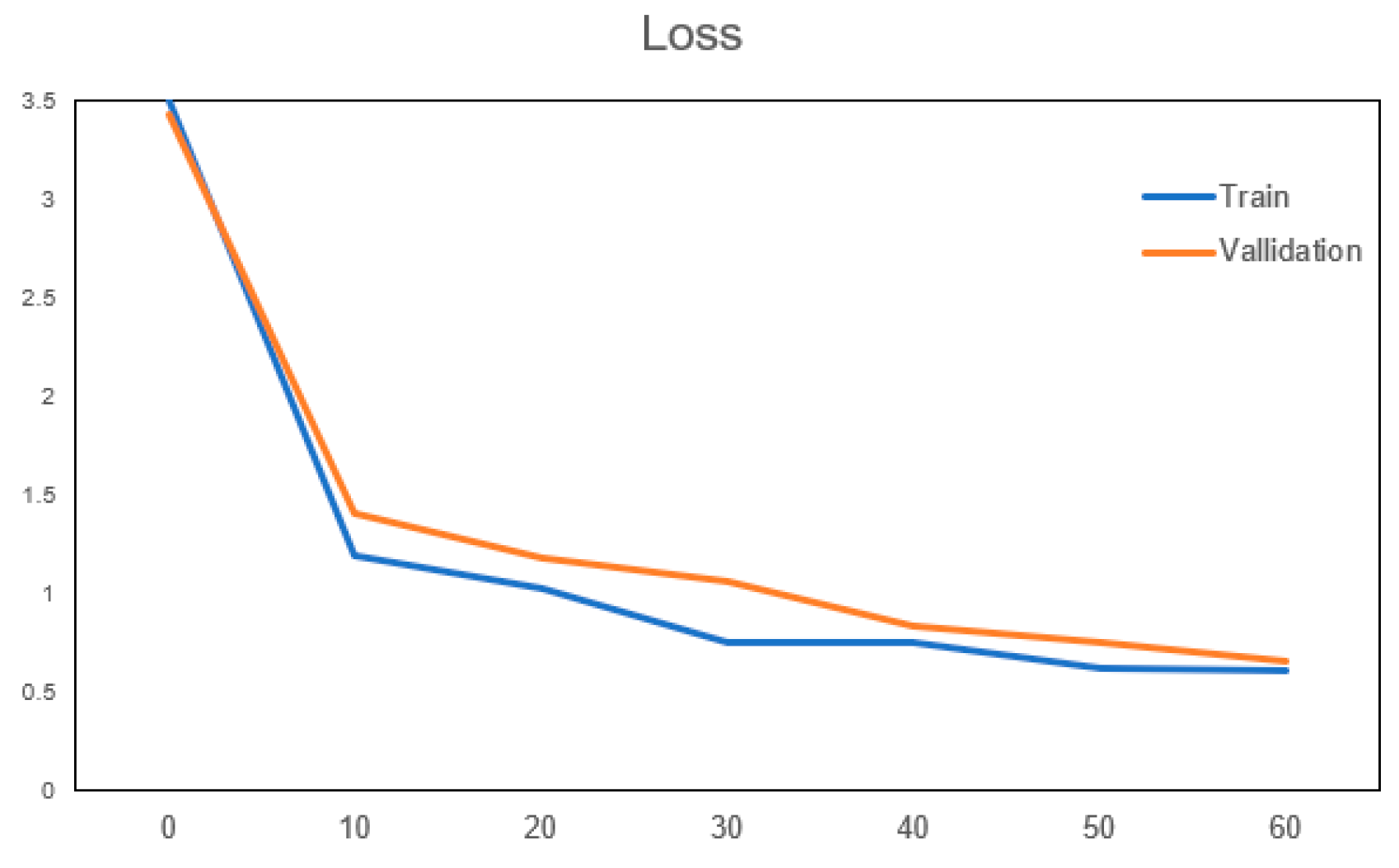
The following shows the training curves of this training model, respectively; the training and validation curves, mainly to verify the accuracy and training loss, and the specific images are shown in Figure 5 and Figure 6 below.
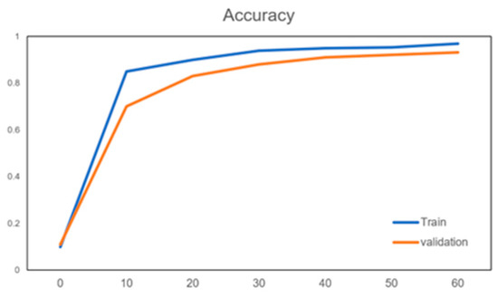
Figure 5.
Accuracy curve.
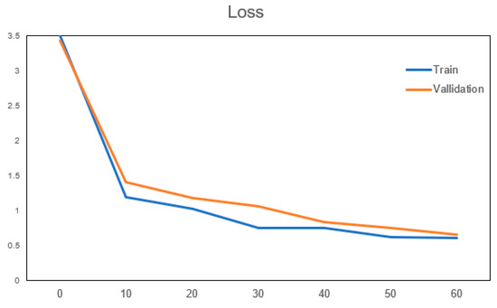
Figure 6.
Loss curve.
It can be seen from the above two pictures that as the number of iterations increases, the model is constantly optimized, the accuracy in the validation set continues to improve, the loss value is gradually reduced, and after verification, the accuracy and loss value above are basically close to the results of the training model. The number of iterations after the increase in the more tend to be more stable; therefore, we believe that the training of the model can satisfy the needs of this and further used it for the following weather recognition that you can deploy on hardware FPGA for acceleration.
4. Design of FPGA Implementation
4.1. System Architecture
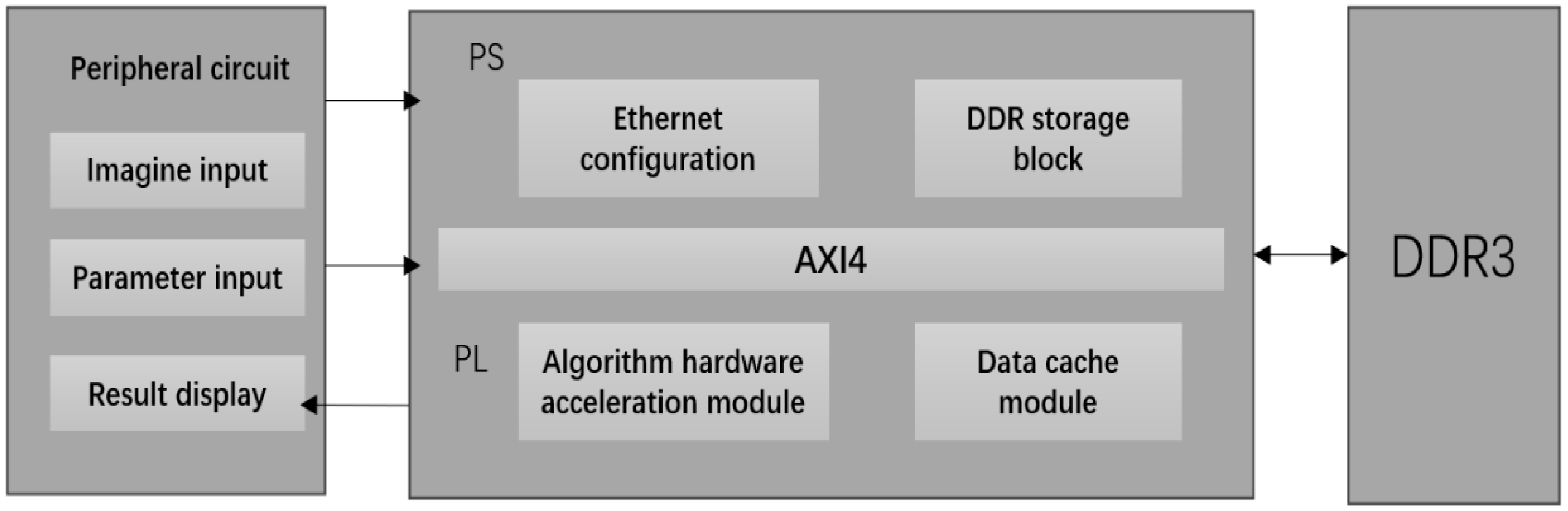
This design is based on a heterogeneous FPGA-development platform, and its main purpose is to fully shorten the forward reasoning time of the neural network model while reducing the BRAM resource occupation. Figure 7 shows the system block diagram of this design. The main institutional components of this design can be seen roughly in Figure 7 below.

Figure 7.
Weather-Net system architecture.
The external functional module includes a model parameter input module, weather-image-acquisition and preprocessing module, and recognition result display module, which is mainly responsible for inputting the processed image data and network parameters into FPGA through the network port and displaying the returned recognition results in real-time. The PL part of FPGA includes the algorithm hardware acceleration module and the data cache module, which is mainly responsible for the design and implementation of the weather recognition algorithm with Verilog language and the formulation of efficient data stream input and the cache form according to the algorithm model structure, so as to give full play to the speed advantage of FPGA parallel computing. The DMA IP core is used to control the data flow between the PL-end and PS-end DDR for high-speed and stable transmission. The PS part includes a DDR storage module and Ethernet configuration module, which is mainly responsible for controlling the input image data and model parameters and configuring the DMA IP core and Ethernet communication.
The actual application scenario of the system is the real-time recognition of multi-section weather images. The specific work-flow is as follows: first, the host computer sends the trained model parameters to the PS terminal of FPGA through the gigabit network port and saves them to the specified address of DDR to complete the initial configuration; then, the host computer preprocesses the acquired multi-channel image data and sends them successively to the PS DDR for caching through the gigabit network port. When the PL terminal operation module starts to work, the model parameters and input images will be sent to the PL terminal through DMA in the form of the AXI_Stream for calculation. Finally, the output result of the computing module will be returned to the upper computer through the PS end Ethernet port.
4.2. Convolutional BLOCK Design
In the Weather-Net network algorithm, the convolution module is the key part to extract image feature information, including the depthwise convolution module, parameter cache module, and pointwise convolution module.
Depthwise convolution is similar to the standard convolution principle, including window sliding, convolution calculation, and computational state control. The window sliding is realized by shift-ram and register. The network input image size is 128 × 128, and the convolution kernel size is 3 × 3; that is, two shift rams are needed, and each depth is set to 128. Convolution calculation is implemented by the Xilinx multiplier IP core. The input data are the quantized 16-bit fixed-point number, and finally, the calculation result is truncated to the corresponding bit width to keep the data bit width consistent. The calculation state control unit is implemented by a finite state machine, including an idle state, data valid, and an invalid state, which is used to intercept valid calculation results and discard some invalid results in the window sliding process. The final result is passed to the data cache module. The parameter data cache module is used to cache the results of the depthwise convolution calculation and pass them to the pointwise convolution module, using on-chip BRAM resources. Similar to depthwise convolution, the pointwise convolution module includes a convolution calculation unit and a calculation state control unit.
The convolution module is the most basic computing unit for FPGA to implement convolution operations, performing dot product operations of two 9-element vectors:
4.3. Data Quantification
The realization of convolutional neural networks in software is realized by floating-point numbers. However, implementing floating-point operations in hardware consumes a large number of multipliers and brings much power consumption. Once the network layer number is very deep, it may lead to the network not being all hardware or high-power consumption. Therefore, if the neural network is built on FPGA, the floating-point number needs to be quantified into a fixed-point number.
This design adopts a 16-bit fixed-point quantization method. The accuracy loss of using 16 bit fixed-point quantization is less than 1%, and in this paper, both the model input eigenvalues and weight parameters are normalized, and their values range from −1 to 1. Therefore, this paper finally chooses to use the 16-bit fixed-point data format and only retains 1 bit as the sign bit, and the remaining 15 bits indicate the decimal places, to minimize the loss of data accuracy, including a 1-bit symbol bit, 5-bit integer bit, and 10-bit decimal bit. The trained network parameters are exported and transformed into binary numbers that can be recognized by FPGA through Python 3.6, which are stored in ROM in advance and called when the convolution operation is performed. For the image data input by the camera, it is first stored in the internal FIFO; then, the normalized input image is quantized based on the lookup table, and finally, the quantized data are stored in the ROM. The final experimental results show that the parameter accuracy loss of the 16-bit quantization method is within 3%.
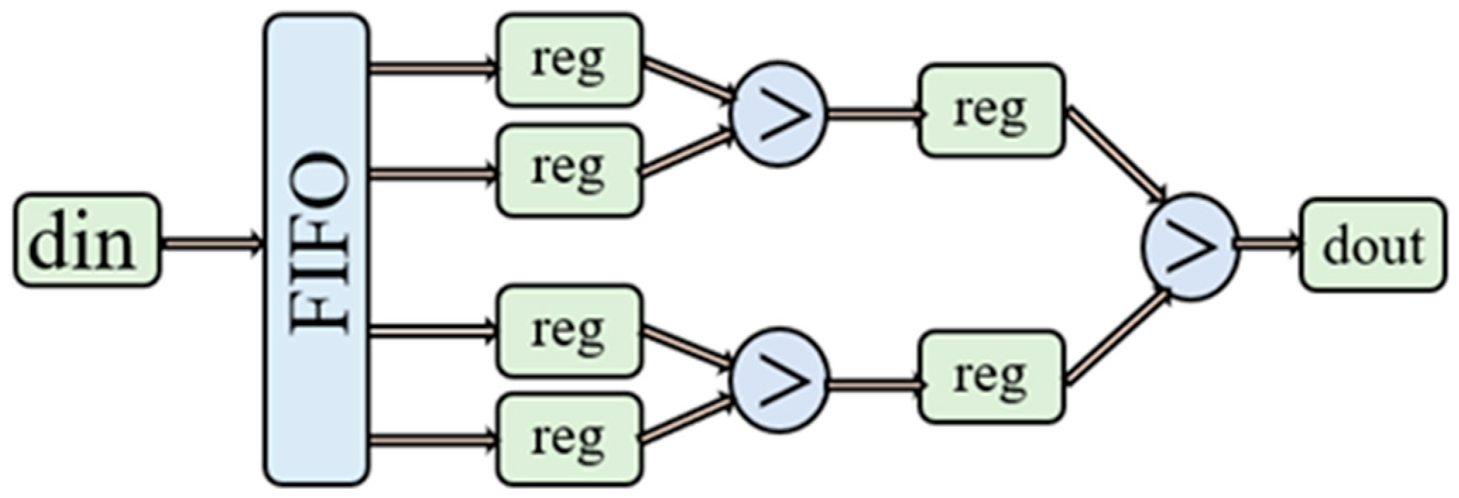
4.4. Max-Pooling Layer Design
The pooling module can downsample the feature image output after the convolution operation and further reduce the number of parameters while maintaining valid image features. A single FIFO buffer unit is used to construct a 2 × 2 size pooling window, and the maximum pooling is achieved by comparing the size relationship between the two datasets. Figure 8 shows a sample of the hardware architecture corresponding to the max-pooling layer.
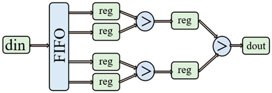
Figure 8.
Hardware architecture of the max-pooling layer using a kernel size of 2 × 2.
Figure 8 mainly wants to show the main structure of the pooling layer.
4.5. Activation Function Design
The main function of the activation function is the ability to perform a non-linear transformation of an arbitrary function based on the input, giving the convolutional neural network the ability to learn additional complex matters. At the same time, the activation function can classify it so that it allows error back propagation to train the network model. ReLU [27], sigmoid, and tanh are some of the commonly used activation functions, with ReLU being the less computationally-intensive activation function as it does not involve the calculation of exponents and divisions.
4.6. Convolutional Neural Network Simulation Waveform
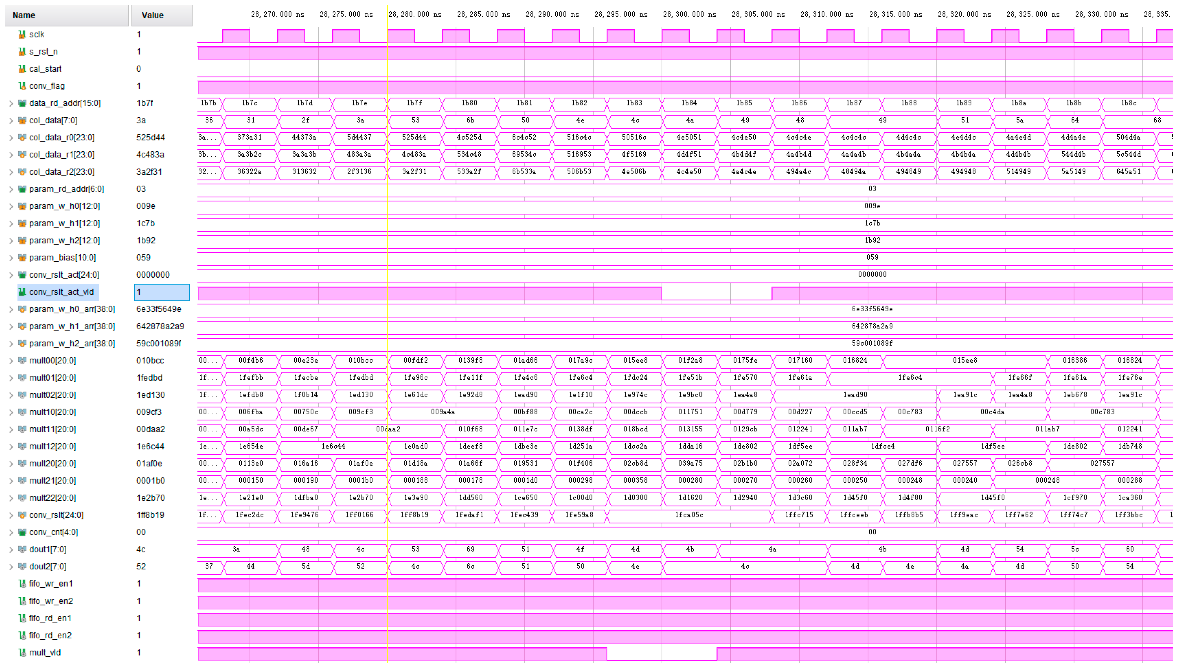
In FPGA hardware design, each convolutional layer, which accounts for more than 90% of the calculation of the algorithm, is realized by the standard convolutional computing unit, and the circuit module of the unit is simulated separately. By adding the input excitation, which is close to the actual use scenario, the calculated output result is observed, and the timing of each control signal is analyzed.
Figure 9 shows the simulation waveform diagram of the standard convolution unit. Input image data and parameter data are added to test the output results of the first layer of the standard convolution. The input clock frequency is 50 MHz, and the input image data size is 128 × 128 × 3. As can be seen from the figure, after the convolution calculation begins, image data and parameter data are successively read into the register cache. When the nine convolution kernel parameters of a channel are read, the parameter register stops updating. After the first feature graph convolution window appears, the operation unit starts to work, and eight convolution sliding window operations will be carried out simultaneously in one clock cycle. Because the addition tree is adopted in this paper to realize the addition of nine numbers, the effective signal of the output result of the operation unit has to lag two clock cycles, and the output result is the result of the multiplication and addition operation of the corresponding data in the window.
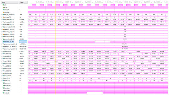
Figure 9.
Simulation waveform of standard convolution unit.
5. FPGA Implementation, Verification, and Results
5.1. FPGA Implementation
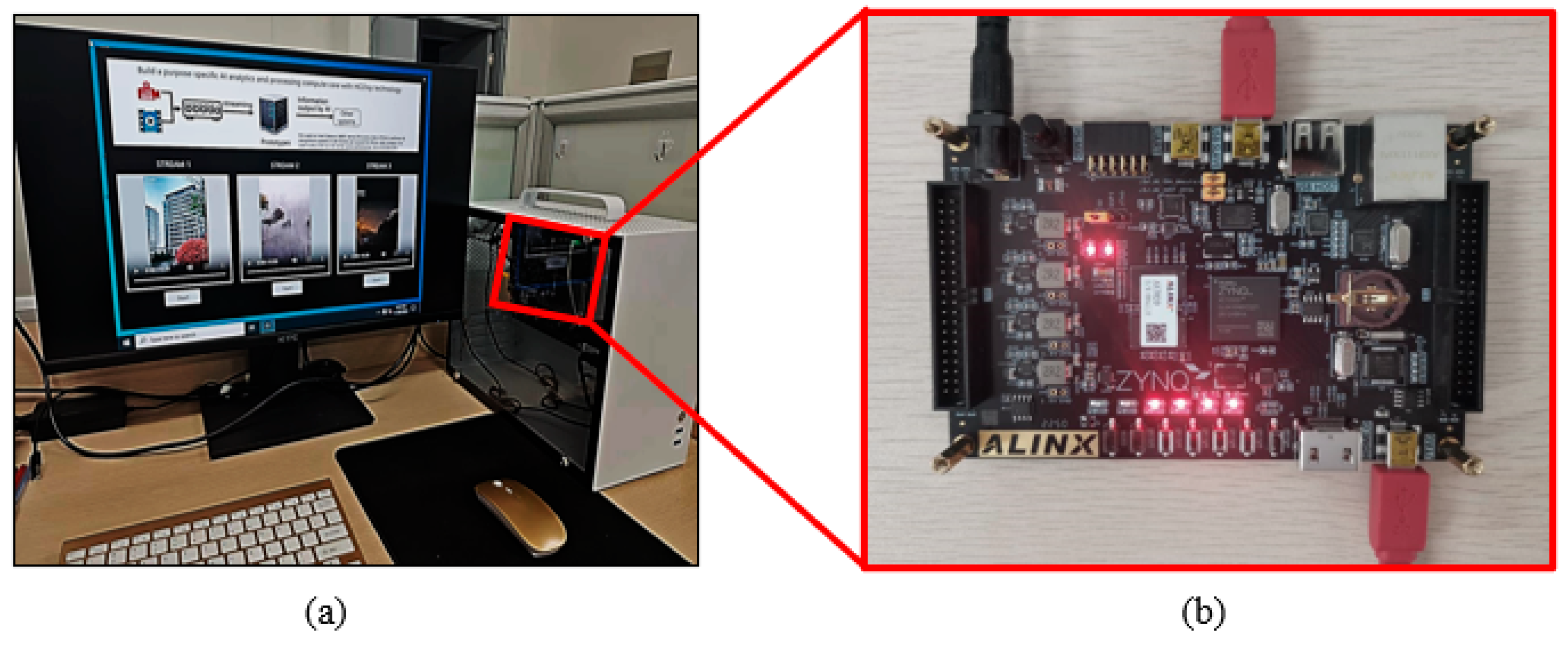
In this paper, when the Weather-Net network algorithm is deployed on FPGA, the selected FPGA chip is Xilinx Zynq-7020. The FPGA is connected to an x86-based host PC via a gigabit Ethernet cable. The platform characteristics are shown in Table 3. And Figure 10 shows the physical picture.
Table 3.
Some specifications of the Zynq-7020 development board.
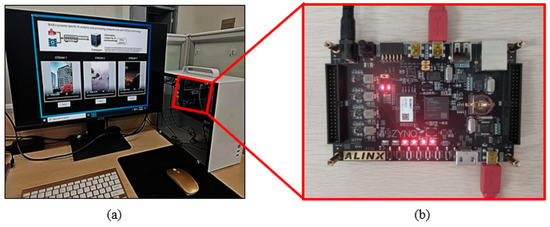
Figure 10.
FPGA verification system: (a) full system operation, including results captured on the monitor. (b) Physical picture of the FPGA platform.
The communication between the host computer and the FPGA uses Ethernet. Compared with serial port and USB2.0 interface transmission, Ethernet has a higher transmission rate, which can fully reduce the data transmission delay and improve the system identification speed. The FPGA development board mainly relies on the physical layer chip to achieve the network communication function. The AX7020 development board supports 10/100/1000 Mbps network transfer rates through a simplified Gigabit independent interface and Zynq 7000 PS data communication.
The specific testing procedure is as follows: first, we trained a traditional convolutional neural network model with the same number of layers as Weather-Net and compared the parameters of the two models with the recognition accuracy. Then, the weather-net is deployed on the FPGA, and the operating parameters are compared with the CPU and GPU. Finally, this design is compared with a number of other similar FPGA designs.
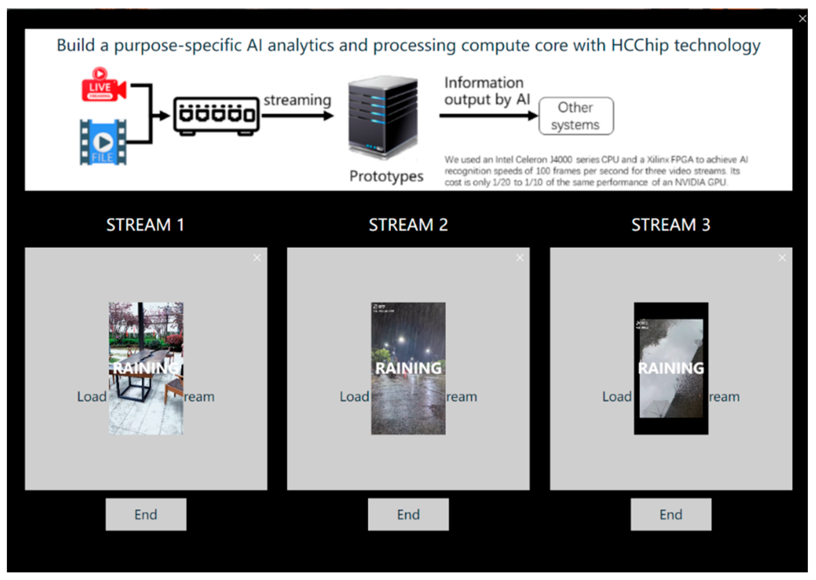
Through the communication between the host computer and the development board, we can realize the communication between the two sides and then complete the identification of different weather types. The specific identification results are shown in Figure 11.
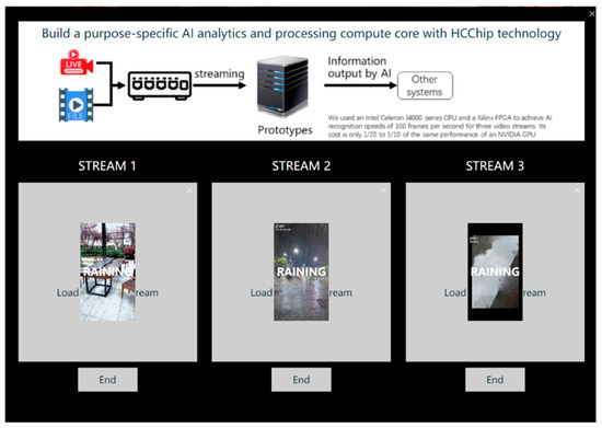
Figure 11.
Weather recognition results of the weather-recognition system.
5.2. FPGA Report
5.2.1. Resource Utilization
The resource consumption is shown in Table 4 below. It can be seen that the design consumes much BRAM resources on the FPGA chip. This is because in the design of this paper, the cache of image data and parameter data all use FPGA on-chip storage resources, which is beneficial to reduce the data transmission delay between each sub-function module, further accelerating the network running speed.
Table 4.
FPGA resource utilization.
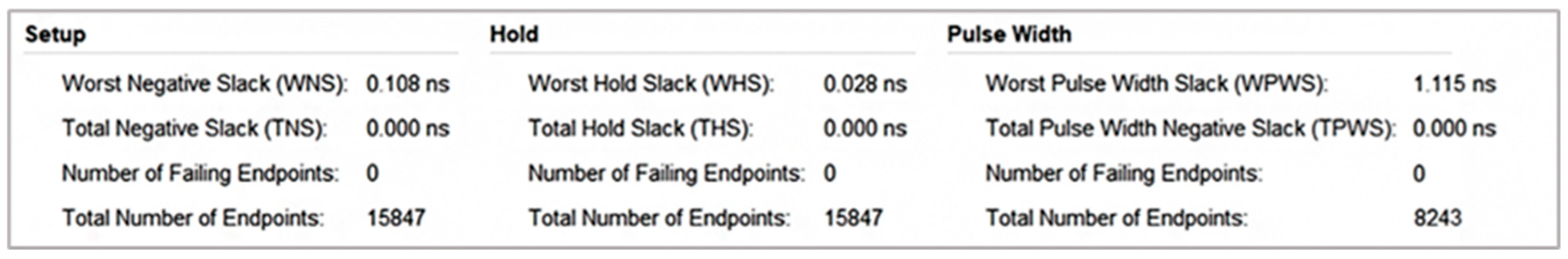
5.2.2. Timing Report
The timing report is shown in Figure 12 below. It can be seen that the setup time slack and hold time slack of the system designed in this paper are positive, indicating that the system timing is good and there are no timing violations.
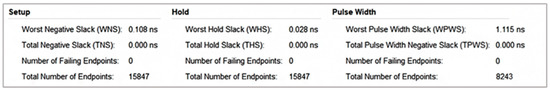
Figure 12.
Timing report.
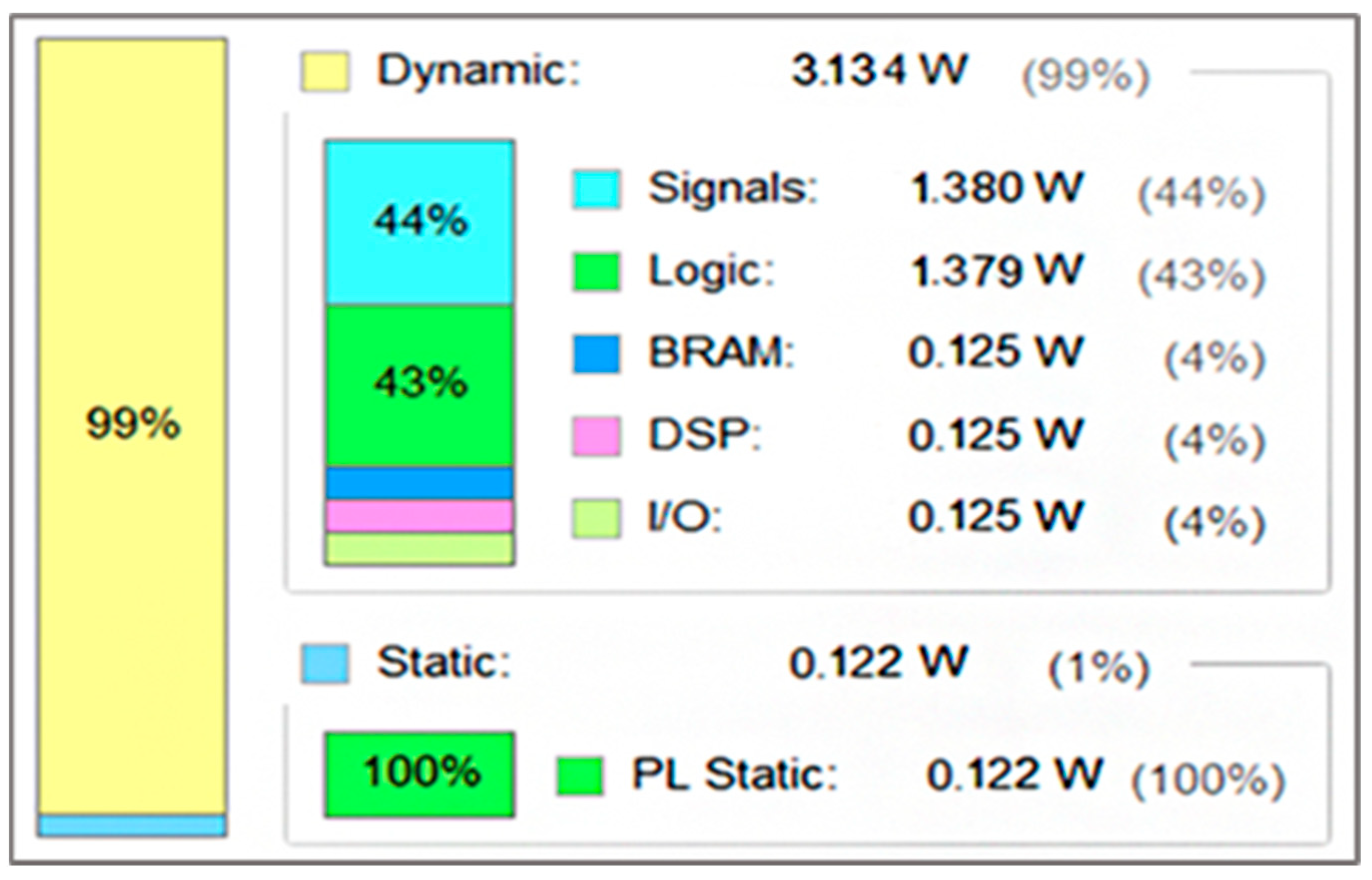
5.2.3. Power Consumption Report
The power consumption report is shown in Figure 13 below. The total power consumption on the FPGA chip is 3.256 W, of which the dynamic power consumption accounts for 99%, and the signal part and the logic part consume more. This is because this work uses FPGA on-chip storage resources to cache image data and network parameters, which can reduce the signal delay between various functional modules. Therefore, the Weather-Net network system consumes a large number of storage resources on the FPGA chip, so the power consumption of these two parts is relatively high.
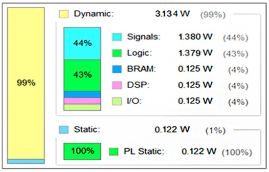
Figure 13.
Power consumption report.
5.3. Comparison of Experimental Results
The comparison results of the parameters and recognition accuracy of the two different convolutional models are shown in Table 5. It can be found that the network model based on the depthwise separable convolution operation can greatly reduce the parameters in the convolution process and has high accuracy.
Table 5.
Comparison of two models.
In Table 6, we compared our work with some existing works on implementing the depthwise separable convolutional neural network on different FPGAs.
Table 6.
Comparison with other FPGA accelerators.
We implement Weather-Net on three platforms, respectively, and compare the test results, including the running time, recognition accuracy, and running power consumption. The experimental results on three platforms are shown in Table 7.
Table 7.
Comparison of Weather-Net implementation on different platforms.
Through the above table, it can be seen that within the acceptable accuracy reduction range (accuracy reduction of 1.4%), compared with CPU, FPGA acceleration performance is ten times its power consumption and is only one quarter; compared to the GPU, FPGA acceleration performance is 1.5 times its power consumption and is only one-tenth. These data show that the FPGA acceleration system designed in this paper has superior acceleration performance and running power consumption while maintaining high recognition accuracy.
6. Conclusions
In this work, we build and train a network model for weather recognition based on depthwise separable convolution and propose a hardware-implementation scheme that can be deployed on FPGA. After experimental verification, the network recognition accuracy can reach 96.8%, and the accuracy is only reduced by 1.4%. FPGA acceleration performance is 108 FPS, and power consumption is only 3.256 W. Through comparative evaluation, the CPU platform acceleration performance is 20 FPS, and power consumption is 13.47 W; the acceleration performance of the GPU platform is 139 FPS, and the power consumption is 27.85 W. Through a comparison, we found that the design of this paper through the FPGA hardware acceleration after the completion of the deployment of the accuracy rate is slightly reduced, but the accuracy rate is reduced by only 1.4%; it is still more than 96%, and we believe that it is still able to meet the unmanned aerial vehicle in the process of real-time monitoring of the outside world environment and the weather status of the function and can assist the unmanned aerial vehicle to complete the flight task, to avoid the damage to the equipment and the limitations of the precision of the equipment. At the same time, after using FPGA hardware deployment acceleration compared to CPU and GPU, this design can simultaneously realize excellent platform acceleration performance and relatively low power consumption, so this design has important value.
Although this FPGA-based weather recognition system has certain advantages in its processing speed and power consumption and has certain application value in recognizing the weather to assist UAVs to fly better and complete their tasks, there are still some aspects that need to be improved and progressed. First of all, the weather recognition of this design is basically based on cloudy, sunny, rainy, and snowy, but the weather that affects the UAV’s flight is not only this; there are still haze and strong wind weather, especially the strong wind weather, and there is no way to use the picture or video-recognition to make an accurate judgment, so this is a place that needs to be improved in the future research. The second is to expand the application of the network model, and we can try to improve it based on a more perfect network model and at the same time expand the dataset to further improve the accuracy. The last thing that is hoped to be improved is the performance of the convolutional computation, and the effort in future research is to use higher-performance algorithms to improve the speed of the convolutional computation. It is hoped that future research will further improve performance and expand more application areas.
Author Contributions
All authors contributed to the study conception and design. Material preparation, data collection, and analysis were performed by L.C., F.L., F.W. and L.L. The first draft of the manuscript was written by F.L. and all authors commented on previous versions of the manuscript. All authors have read and agreed to the published version of the manuscript.
Funding
No funding was received to assist with the preparation of this manuscript.
Data Availability Statement
The data that support the findings of this study are available from the corresponding author upon reasonable request.
Conflicts of Interest
The authors have no competing interests to declare that are relevant to the content of this article.
References
- Cai, Z.; Jiang, F.; Chen, J.; Jiang, Z.; Wang, X. Weather condition dominates regional PM2.5 pollutions in the eastern coastal provinces of China during winter. Aerosol Air Qual. Res. 2018, 18, 969–980. [Google Scholar] [CrossRef]
- Mohan, P.; Patil, K.K. Deep learning based weighted SOM to forecast weather and crop prediction for agriculture application. Int. J. Intell. Eng. Syst 2018, 11, 167–176. [Google Scholar] [CrossRef]
- Li, Z.; Zhong, Y.; Chen, J.; Chen, Y. Multi-class weather classification based on multi-feature weighted fusion method. In IOP Conference Series: Earth and Environmental Science; IOP Publishing: Bristol, UK, 2020; Volume 558, p. 042038. [Google Scholar]
- Lu, C.; Lin, D.; Jia, J.; Tang, C.-K. Two-class weather classification. In Proceedings of the IEEE Conference on Computer Vision and Pattern Recognition, Columbus, OH, USA, 23–28 June 2014; pp. 3718–3725. [Google Scholar]
- Zhao, B.; Li, X.; Lu, X.; Wang, Z. A CNN–RNN architecture for multi-label weather recognition. Neurocomputing 2018, 322, 47–57. [Google Scholar] [CrossRef]
- Katsura, H.; Miura, J.; Hild, M.; Shirai, Y. A view-based outdoor navigation using object recognition robust to changes of weather and seasons. J. Robot. Soc. Jpn. 2005, 23, 75–83. [Google Scholar] [CrossRef]
- Zhu, Z.; Zhuo, L.; Qu, P.; Zhou, K.; Zhang, J. Extreme weather recognition using convolutional neural networks. In Proceedings of the 2016 IEEE International Symposium on Multimedia (ISM), San Jose, CA, USA, 11–13 December 2016; IEEE: New York, NY, USA, 2016; pp. 621–625. [Google Scholar]
- Zhu, Z.; Li, J.; Zhuo, L.; Zhang, J. “Extreme weather recognition using a novel fine-tuning strategy and optimized GoogLeNet. In Proceedings of the 2017 International Conference on Digital Image Computing: Techniques and Applications (DICTA), Sydney, Australia, 29 November–1 December 2017; IEEE: New York, NY, USA, 2017; pp. 1–7. [Google Scholar]
- Liu, W.; Yang, Y.; Wei, L. Weather recognition of street scene based on sparse deep neural networks. J. Adv. Comput. Intell. Intell. Inform. 2017, 21, 403–408. [Google Scholar] [CrossRef]
- Hubara, I.; Courbariaux, M.; Soudry, D.; El-Yaniv, R.; Bengio, Y. Quantized neural networks: Training neural networks with low precision weights and activations. J. Mach. Learn. Res. 2017, 18, 6869–6898. [Google Scholar]
- Denton, E.L.; Zaremba, W.; Bruna, J.; LeCun, Y.; Fergus, R. Exploiting linear structure within convolutional networks for efficient evaluation. Adv. Neural Inf. Process. Syst. 2014, 27, 1269–1277. [Google Scholar]
- Han, S.; Mao, H.; Dally, W.J. Deep compression: Compressing deep neural networks with pruning, trained quantization and huffman coding. arXiv 2015, arXiv:1510.00149. [Google Scholar]
- Iandola, F.N.; Han, S.; Moskewicz, M.W.; Ashraf, K.; Dally, W.J.; Keutzer, K. SqueezeNet: AlexNet-level accuracy with 50x fewer parameters and <0.5 MB model size. arXiv 2016, arXiv:1602.07360. [Google Scholar]
- Howard, A.G.; Zhu, M.; Chen, B.; Kalenichenko, D.; Wang, W.; Weyand, T.; Andreetto, M.; Adam, H. Mobilenets: Efficient convolutional neural networks for mobile vision applications. arXiv 2017, arXiv:1704.04861. [Google Scholar]
- Zhang, X.; Zhou, X.; Lin, M.; Sun, J. Shufflenet: An extremely efficient convolutional neural network for mobile devices. In Proceedings of the IEEE Conference on Computer Vision and Pattern Recognition, Salt Lake City, UT, USA, 18–23 June 2018; IEEE: New York, NY, USA, 2018; pp. 6848–6856. [Google Scholar]
- Chollet, F. Xception: Deep learning with depthwise separable convolutions. In Proceedings of the IEEE Conference on Computer Vision and Pattern Recognition, Honolulu, HI, USA, 21–26 July 2017; IEEE: New York, NY, USA, 2017; pp. 1251–1258. [Google Scholar]
- Simonyan, K.; Zisserman, A. Very deep convolutional networks for large-scale image recognition. arXiv 2014, arXiv:1409.1556. [Google Scholar]
- Chetlur, S.; Woolley, C.; Vandermersch, P.; Cohen, J.; Tran, J.; Catanzaro, B.; Shelhamer, E. cuDNN: Efficient primitives for deep learning. arXiv 2014, arXiv:1410.0759. [Google Scholar]
- Zhang, C.; Li, P.; Sun, G.; Guan, Y.; Xiao, B.; Cong, J. Optimizing FPGA-based accelerator design for deep convolutional neural networks. In Proceedings of the 2015 ACM/SIGDA International Symposium on Field-Programmable Gate Arrays, Monterey, CA, USA, 12–14 February 2023; pp. 161–170. [Google Scholar]
- Luo, S.; Zhang, G.; Wu, C.; Khan, S.U.; Li, K. Boafft: Distributed deduplication for big data storage in the cloud. IEEE Trans. Cloud Comput. 2015, 8, 1199–1211. [Google Scholar] [CrossRef]
- Lagorio, A.; Grosso, E.; Tistarelli, M. Automatic detection of adverse weather conditions in traffic scenes. In Proceedings of the 2008 IEEE Fifth International Conference on Advanced Video and Signal Based Surveillance, Santa Fe, NM, USA, 1–3 September 2008; IEEE: New York, NY, USA, 2008; pp. 273–279. [Google Scholar]
- Chen, Z.; Yang, F.; Lindner, A.; Barrenetxea, G.; Vetterli, M. How is the weather: Automatic inference from images. In Proceedings of the 2012 19th IEEE International Conference on Image Processing, Orlando, FL, USA, 30 September–3 October 2012; IEEE: New York, NY, USA, 2012; pp. 1853–1856. [Google Scholar]
- Roser, M.; Moosmann, F. Classification of weather situations on single color images. In Proceedings of the IEEE Intelligent Vehicles Symposium, Eindhoven, The Netherlands, 4–6 June 2008; IEEE: New York, NY, USA, 2008; pp. 798–803. [Google Scholar]
- Zhang, Z.; Ma, H. Multi-class weather classification on single images. In Proceedings of the 2015 IEEE International Conference on Image Processing (ICIP), Quebec City, QC, Canada, 27–30 September 2015; IEEE: New York, NY, USA, 2015; pp. 4396–4400. [Google Scholar]
- Sifre, L.; Mallat, S. Rigid-motion scattering for texture classification. arXiv 2014, arXiv:1403.1687. [Google Scholar]
- Lin, D.; Lu, C.; Huang, H.; Jia, J. RSCM: Region selection and concurrency model for multi-class weather recognition. IEEE Trans. Image Process. 2017, 26, 4154–4167. [Google Scholar] [CrossRef]
- Nwankpa, C.; Ijomah, W.; Gachagan, A.; Marshall, S. Activation functions: Comparison of trends in practice and research for deep learning. arXiv 2018, arXiv:1811.03378. [Google Scholar]
- Lin, Y.; Zhang, Y.; Yang, X. A Low Memory Requirement MobileNets Accelerator Based on FPGA for Auxiliary Medical Tasks. Bioengineering 2022, 10, 28. [Google Scholar] [CrossRef] [PubMed]
- Li, G.; Zhang, J.; Zhang, M.; Wu, R.; Cao, X.; Liu, W. Efficient depthwise separable convolution accelerator for classification and UAV object detection. Neurocomputing 2022, 490, 1–16. [Google Scholar] [CrossRef]
- Ding, W.; Huang, Z.; Huang, Z.; Tian, L.; Wang, H.; Feng, S. Designing efficient accelerator of depthwise separable convolutional neural network on FPGA. J. Syst. Archit. 2019, 97, 278–286. [Google Scholar] [CrossRef]

Disclaimer/Publisher’s Note: The statements, opinions and data contained in all publications are solely those of the individual author(s) and contributor(s) and not of MDPI and/or the editor(s). MDPI and/or the editor(s) disclaim responsibility for any injury to people or property resulting from any ideas, methods, instructions or products referred to in the content. |
© 2025 by the authors. Licensee MDPI, Basel, Switzerland. This article is an open access article distributed under the terms and conditions of the Creative Commons Attribution (CC BY) license (https://creativecommons.org/licenses/by/4.0/).