Abstract
We propose an autofocusing algorithm to obtain, relatively accurately, the 3D position of each particle, particularly its axial location, and particle number of a dense transparent particle solution via its hologram. First, morphological analyses and constrained intensity are used on raw reconstructed images to obtain information on candidate focused particles. Second, axial resolution is used to obtain the real focused particles. Based on the mean intensity and equivalent diameter of each candidate focused particle, all focused particles are eventually secured. Our proposed method can rapidly provide relatively accurate ground-truth axial positions to solve the autofocusing problem that occurs with dense particles.
1. Introduction
Digital holography (DH) is a sophisticated optical technology that specializes in capturing and reconstructing the optical information on three-dimensional (3D) objects. Unlike conventional microscopy, which is limited to imaging a single plane, digital holographic microscopy (DHM) is able to capture an entire volume and reconstruct every plane of this volume. Recently, the challenges of sizing, counting, and locating in situ micro-objects (particles, bubbles, or microorganisms) have garnered significant attention from researchers. This interest has been particularly driven by the development of in-line DH and its potential as an alternative to conventional microscopy [1,2]. In both DH and DHM, autofocusing is a crucial technique used to precisely determine the location of an object. While experimental configurations can achieve autofocusing [3,4], it is more commonly realized through computational algorithms, including the methods based on image sharpness [5,6], structure tensor [7], edge sparsity [8], magnitude differential [9], etc.
A number of researchers [10,11,12,13] have employed spherical waves to illuminate particles suspended in water. They determined the position and measured the size of each particle using a captured hologram. The experimental configuration achieved magnification of the target object. However, this approach not only reduces the field of view (FOV), but also significantly impacts the accuracy of both the particle count and their locations along the z-axis, depending on the chosen depth spacing. On the other hand, Tian et al. [14] investigated bubbles in water and employed the minimum intensity as a focus metric to detect the edges of bubbles, thereby accurately determining the location of each bubble, particularly its axial position. However, despite the faster processing speed of their proposed approach, the location information obtained is inaccurate. Moreover, when several bubbles are clustered together, they are mistakenly identified as a single bubble. These conventional methods, which are subject to the diffraction limit, cause severe defocused image problems if the ground-truth z-position of each micro-object is unknown. This ultimately leads to inaccuracies in determining the micro-objects on the mount and their locations. Later on, Lang et al. [15] utilized the Q value as the focus metric to recognize the best axial location for plankton; however, this focus metric is not suitable for numerous particles, especially dense particles in DH.
Compressive models leveraging sparsity have demonstrated remarkable performance in addressing noise and ghost artifacts by reformulating the hologram reconstruction problem as a regularized nonlinear optimization task. Brady et al. [16] introduced a compressive sensing algorithm for DH and showed that decompressive inference can infer multidimensional objects from a single 2D hologram. Liu et al. [17,18] applied compressive holography to object localization, achieving significant improvements in transverse localization accuracy when the solution is sparse in its derivatives. Chen et al. [19] further explored this domain by using a plane wave to illuminate bubbles; however, their method struggled with distinguishing bubbles that were completely or partially overlapped along the z-axis and could not effectively process dense particle fields. A common thread among these studies was the use of total variation regularizers. In contrast, Li et al. [20] applied a 3-D hybrid-Weickert nonlinear diffusion regularizer to DH, which successfully located small-sized transparent scattering particles that overlapped along the z-axis and removed defocused images. As a result, similar autofocusing for multiple micro-objects was achieved while simultaneously eliminating defocused images. Despite these advancements, all of the aforementioned methods have their drawbacks, including slow processing speed, the inability to process dense particles due to a sparse prior, difficulty in fine-tuning the parameters, among others.
With the recent advancements in machine learning, several innovative approaches have been developed to address autofocusing and 3D reconstruction challenges in DH. Ren et al. [21] efficiently employed convolutional neural networks (CNN) to reformulate autofocusing as a classification problem, thereby providing approximations of the focusing distance for each classification. This method is particularly well suited for single large objects, although it does not require reconstructing images. Lee et al. [22] proposed an alternative approach in which the centroid of each particle is first determined and then the cropped hologram of each particle is fed into a CNN to obtain depth information. Shao et al. [23] and Wu et al. [24] utilized a modified U-net network to extract 3D morphological information of all particles, including their 3D positions, sizes, and shapes, primarily from holograms. Li et al. [25] and Hao et al. [26] combined Dense Block and U-net to achieve 3D particle distribution with particle sizes particularly from reconstructed images. Ou et al. [27] employed a modified CNN architecture to predict particle numbers from holograms. However, this approach is incapable of obtaining the 3D positions of particles, especially their axial positions.
In this study, we propose an autofocusing method based on morphological analyses and axial resolution to obtain, relatively accurately, the 3D position of each particle, particularly its axial location, and the particle number of a dense transparent particle solution via a hologram. Our proposed method has two main components. First, morphological analyses and constrained intensity are used on raw reconstructed images, from which information on candidate focused particles is obtained and saved in one matrix. Second, axial resolution is used to obtain the real focused particles from the aforementioned matrix. For the focus metric, we propose using the product of the mean intensity and equivalent diameter of each candidate focused particle. Eventually, we are able to secure all focused particles for one hologram. In our experiments, we used particles located at fixed distances and in a particle solution that was filled in a cuvette to examine and verify the proposed method.
The remainder of this paper is organized as follows. Section 2 introduces the principles. Section 3 presents the methodology, in which the description of the algorithm is a key point. Section 4 discusses the experimental results and analyses. Finally, Section 5 presents the conclusions of our study.
2. Principles
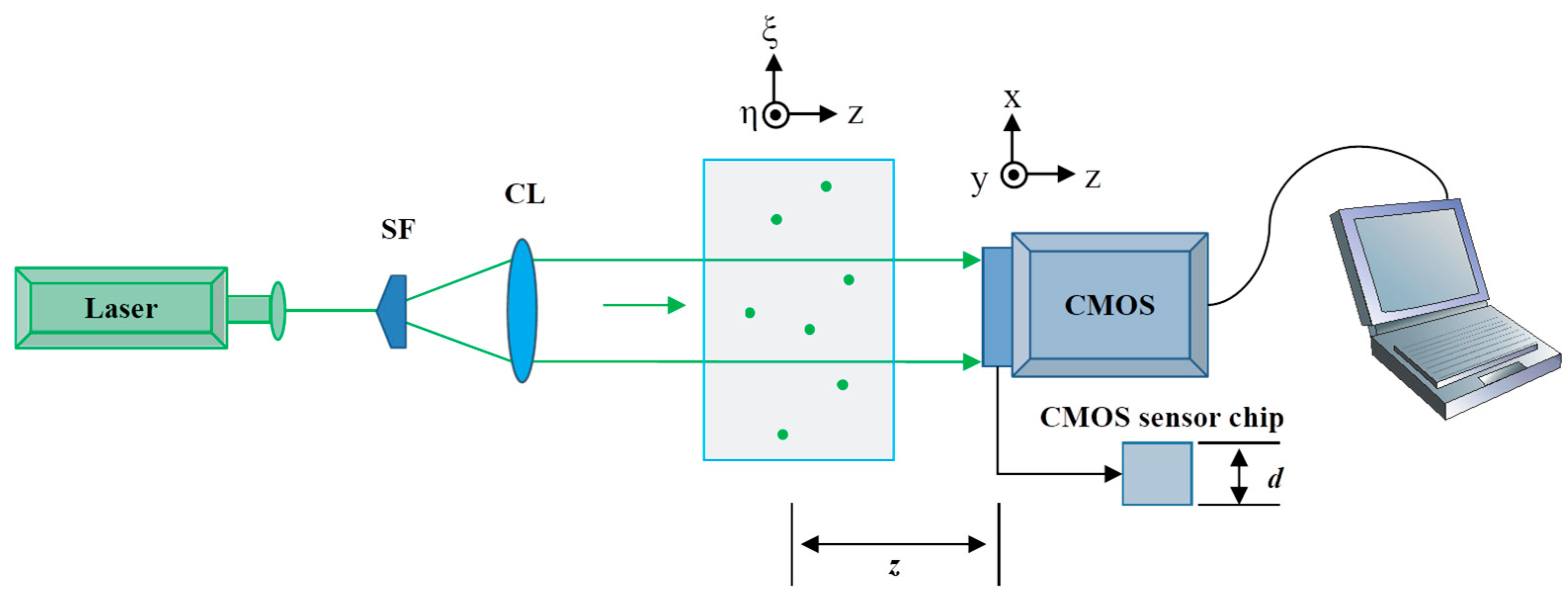
Herein, it is assumed there are a large number of transparent particles suspended in Milli-Q water, all with a uniform size (diameter) denoted by , where i = 1, 2, … m. A plane wave with wavelength illuminates these particles, and holograms of the 3D information of all the particles in the entire volume are captured using a complementary metal oxide semiconductor (CMOS) camera, as shown in Figure 1. If each particle is suspended at a distance from the image sensor chip (hologram plane), the Fresnel diffraction [28] for each particle can be mathematically expressed as follows:
where denotes the lateral coordinates of the particle position, signifies the spatial frequency domain, denotes the hologram plane, and denote the complex amplitude and conjugate, respectively, of the hologram , and n indicates the noise induced by the optical system (including high-frequency speckle noise, the diffraction patterns of dust or bubbles in the optical path, among others). Owing to the use of a plane wave as the reference beam, the amplitude of the reference beam . Therefore, the hologram can be rewritten as shown in Equation (4), in which .

Figure 1.
Schematic diagram of in-line digital holographic setup for capturing holograms of multiple particles (SF: spatial filter; CL: collimating lens; z: transmission distance between object plane and hologram plane; d: height of CMOS sensor chip).
3. Methodology
3.1. Axial Resolution
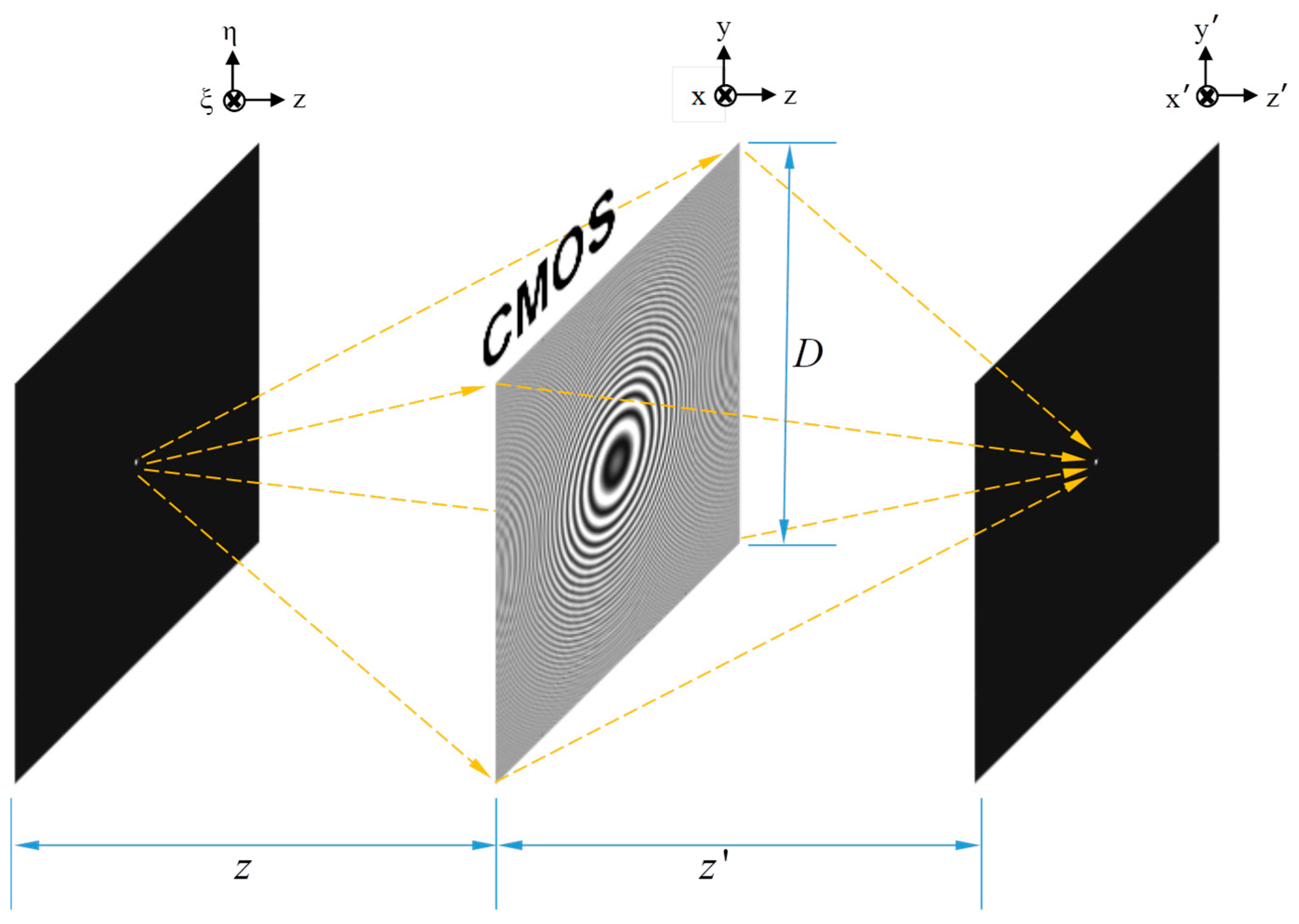
In a digital holographic system, assume a point light source with a wavelength is located at a distance away from the CMOS sensor (hologram plane) whose size is and pixel pitch is ; therefore, the height of the hologram is . The schematic diagram is depicted in Figure 2, where denote the lateral coordinates of the object’s position; denote the hologram plane; and denote the plane of the reconstructed image. Therefore, the numerical aperture (NA) of the hologram and sensor are given by Equation (5) and Equation (6), respectively. The smaller NA is chosen as the real NA between and , and is renamed .
where denotes choosing the minimum one. The lateral resolution of the digital holographic system is given by Equation (8), and the axial resolution of the hologram is presented in Equation (9) [29,30].
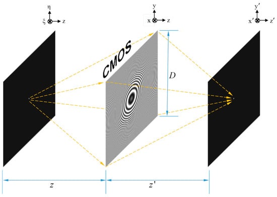
Figure 2.
Schematic diagram of holographic system for one point.
3.2. Constrained Intensity for Each Candidate Focused Particle
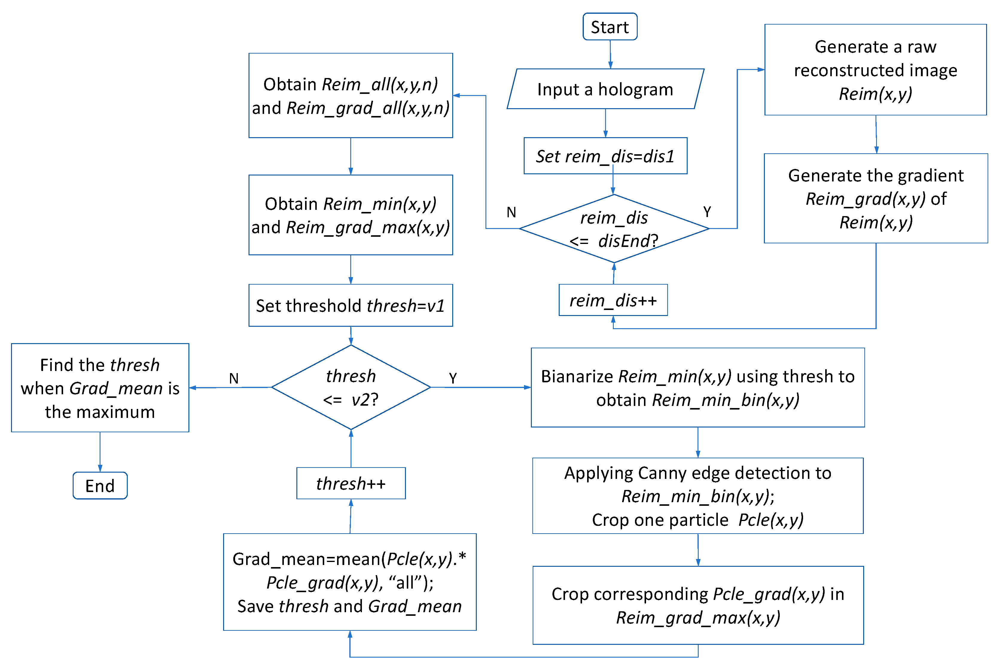
Subsequently, we must find out a suitable threshold value to recognize the candidate focused particles in each raw reconstructed image generated from the hologram, in which there are a large number of transparent particles. A flowchart illustrating the procedure of how to find a suitable constrained intensity is shown in Figure 3. First, a stack of raw reconstructed images and corresponding gradient images is generated. Subsequently, the minimum value along the z-axis is extracted from to obtain a synthetic minimum intensity image . Similarly, the maximum value along the z-axis is extracted from to obtain a synthetic maximum gradient image . Then, a threshold in the range of is sequentially set to binarize to obtain a binarization image . Canny edge detection is applied to obtain the edge of each particle. Afterward, one particle is cropped from , and the corresponding position in the is multiplied to obtain the mean value, applying . The threshold is considered to be suitable when reaches the maximum value. Several other particles are similarly chosen, and their corresponding suitable thresholds are similarly calculated. Finally, among these, the minimum threshold is selected; this is the most suitable constrained intensity for the candidate focused particles [31].
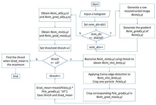
Figure 3.
Flowchart of procedure to find most suitable constrained intensity for candidate focused particles.
3.3. Description of Algorithm
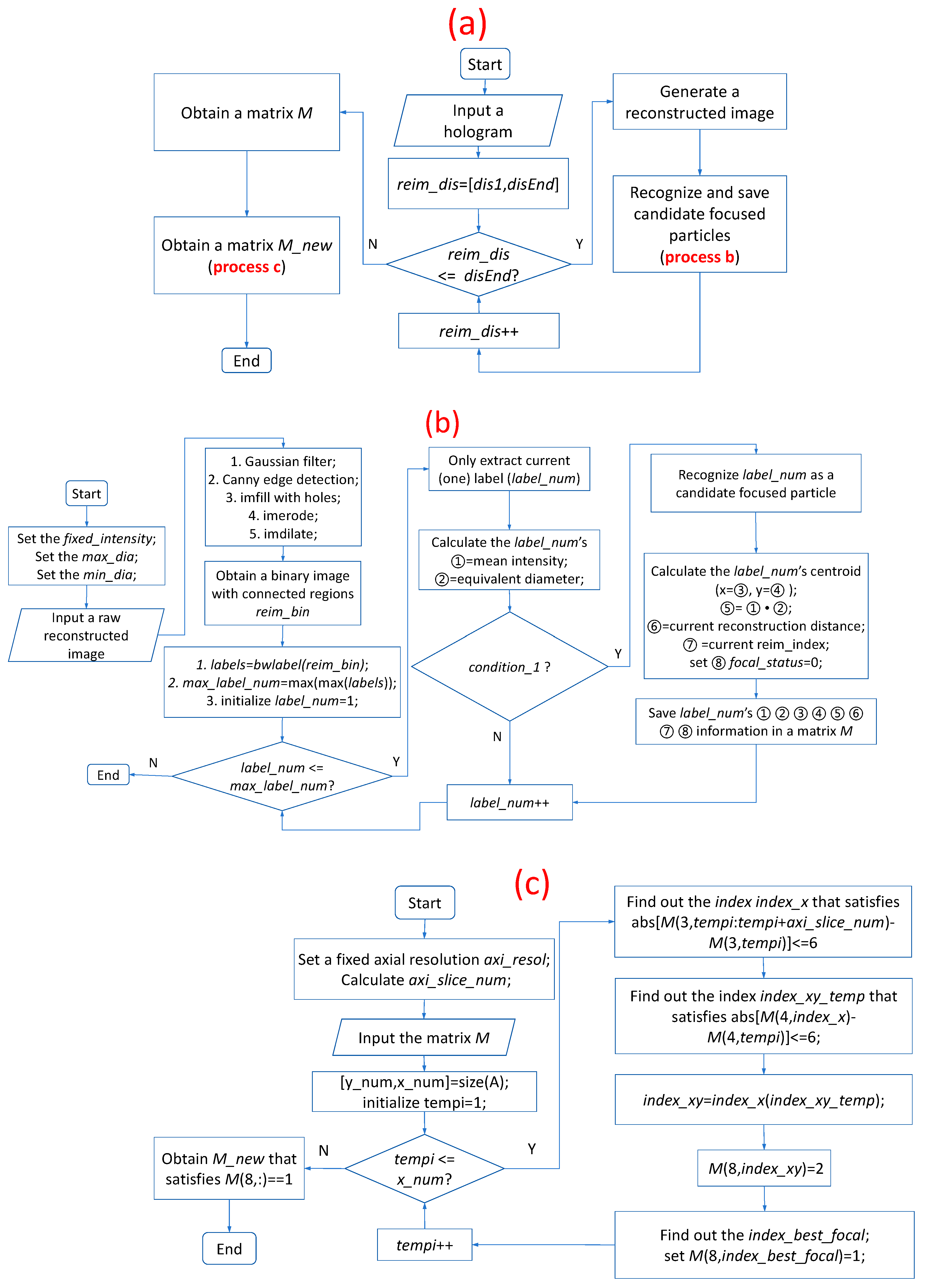
It is assumed that the hologram is captured using an optical setup, the schematic of which is shown in Figure 1. The axial resolution is obtained as described in Section 3.1 to set the smallest axial distance by which to recognize a focused particle. A flowchart of the overall procedure is shown in Figure 4a, which references process b and process c. Process b, shown in Figure 4b, recognizes and saves the information on each candidate focused particle in matrix M, whereas process c, shown in Figure 4c, recognizes the focused particles from matrix M and saves their information in matrix M_new.
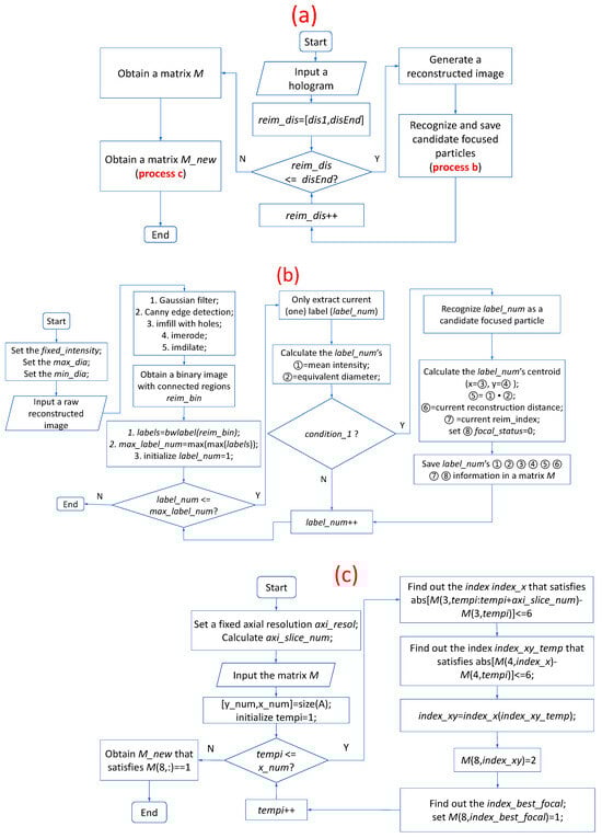
Figure 4.
Flowcharts of (a) overall process to obtain all focused particles’ information, (b) process to obtain and save all candidate focused particles’ information in matrix M, and (c) process to determine and save the focused particles in matrix M_new.
As depicted in Figure 4a, the reconstruction distance range with a fixed reconstruction depth spacing is settled first, and a series of raw reconstructed images are generated using the back Fresnel propagation method. Subsequently, process b is implemented to obtain the matrix M, in which the information of all candidate focused particles are saved. Finally, process c is implemented to obtain the matrix M_new, in which the informtion of all focused particles are saved. The matrix M_new is a subset of the matrix M.
In process b, the constrained intensity fixed_intensity is calculated as described in Section 3.2 to constrain the intensity of each candidate focused particle. The particle diameters are in the range of µm, which is known. After Gaussian filtering, Canny edge detection, hole filling, erosion, and dilation of morphological operations are sequentially applied on one raw reconstructed image, a binary image with connected regions is obtained. The function bwlabel is utilized to extract all of the connected regions (labels), and the number of labels is obtained. Subsequently, all of the labels are traversed. First, the current label label_num is extracted in isolation, and its mean intensity (①) and equivalent diameter (②) are calculated using the function regionprops. If ① is smaller than fixed_intensity and ② is in the range , which is renamed to ‘condition_1’ in Figure 4b, label_num is recognized as a candidate focused particle. Subsequently, its centroid (x, y) (③ and ④), and are continually calculated; the reconstruction distance (⑥) and reim_index (⑦) are saved; and focal_status is set to 0 (⑧). Then, for candidate focused particle label_num, the values of ①, ②, ③, ④, ⑤, ⑥, ⑦, and ⑧ are all saved in matrix M. Eventually, we obtain a matrix M containing the information of all candidate focused particles via process b.
In process c, the focused particles from matrix M are extracted and the information, ①, ②, ③, ④, ⑤, ⑥, ⑦, and ⑧, of each focused particle are saved into a new matrix M_new, except that ⑧ focal_status is made equal to 1. The axial resolution axi_resol is obtained, as described in Section 3.1, to set the smallest axial distance by which to recognize a focused particle. The corresponding axi_slice_num is also calculated. We obtain the number (x_num) of all candidate focused particles from matrix M. Then, we traverse all of these candidate focused particles. During the process, we set tempi = 1:x_num, extract the information of particle tempi, and find the index index_xy in M wherein the particles whose x and y axes of the centroid and the tempi particle’s x and y axes of the centroid are both less than six pixels, in a series of the reconstructed images, from tempi to . Meanwhile, focal_status is set to , to indicate that these candidate focused particles in matrix M have already been traversed. Eventually, we find the index index_best_focal that satisfies the condition that is the minimum value in , and focal_status (⑧) is set to be equal to . Finally, we obtain a new matrix M_new composed of all of the focused particles. As the candidate focused particles in matrix M are traversed, focal_status is made equal to 2, to indicate that the corresponding particle has already traversed; indicates that the corresponding particle has not yet been traversed, whereas indicates that the front axi_slice_num reconstructed images of the corresponding particle have already been traversed and it is a focused particle, but the rear axi_slice_num reconstructed images of the corresponding particle have not yet been traversed. Therefore, if the focal_status of particle tempi is equal to 0 or 1, the particle should be traversed. After all particles are traversed in matrix M, the particles whose focal_status are equal to 1 are the focused particles. For the focus metric, we propose using the minimum of product (⑤) of the mean intensity (①) and equivalent diameter (②), which is easier for processing multiple particles in DH, according to the experimental results.
4. Experimental Results and Analyses
4.1. Particles in Two Layers
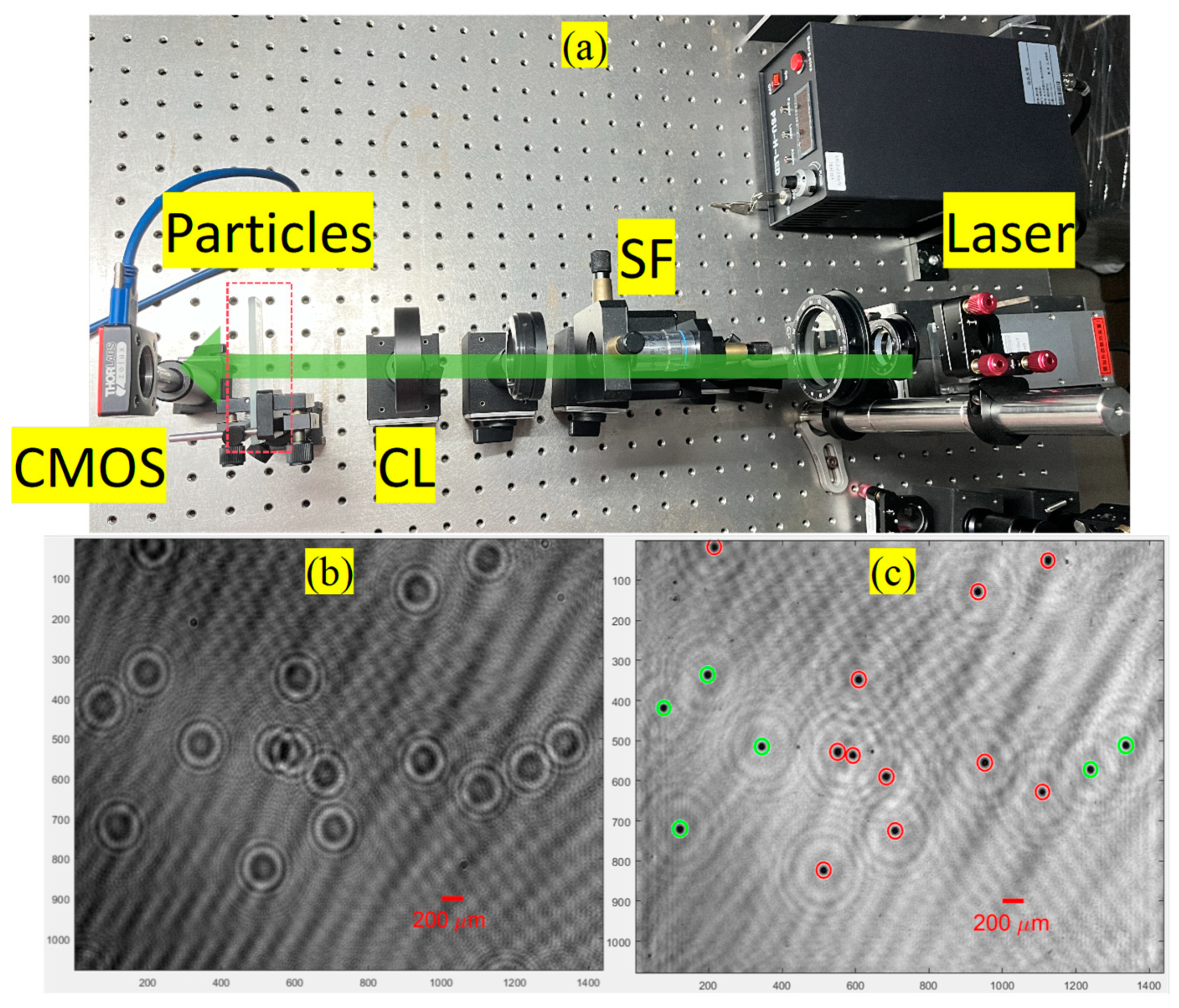
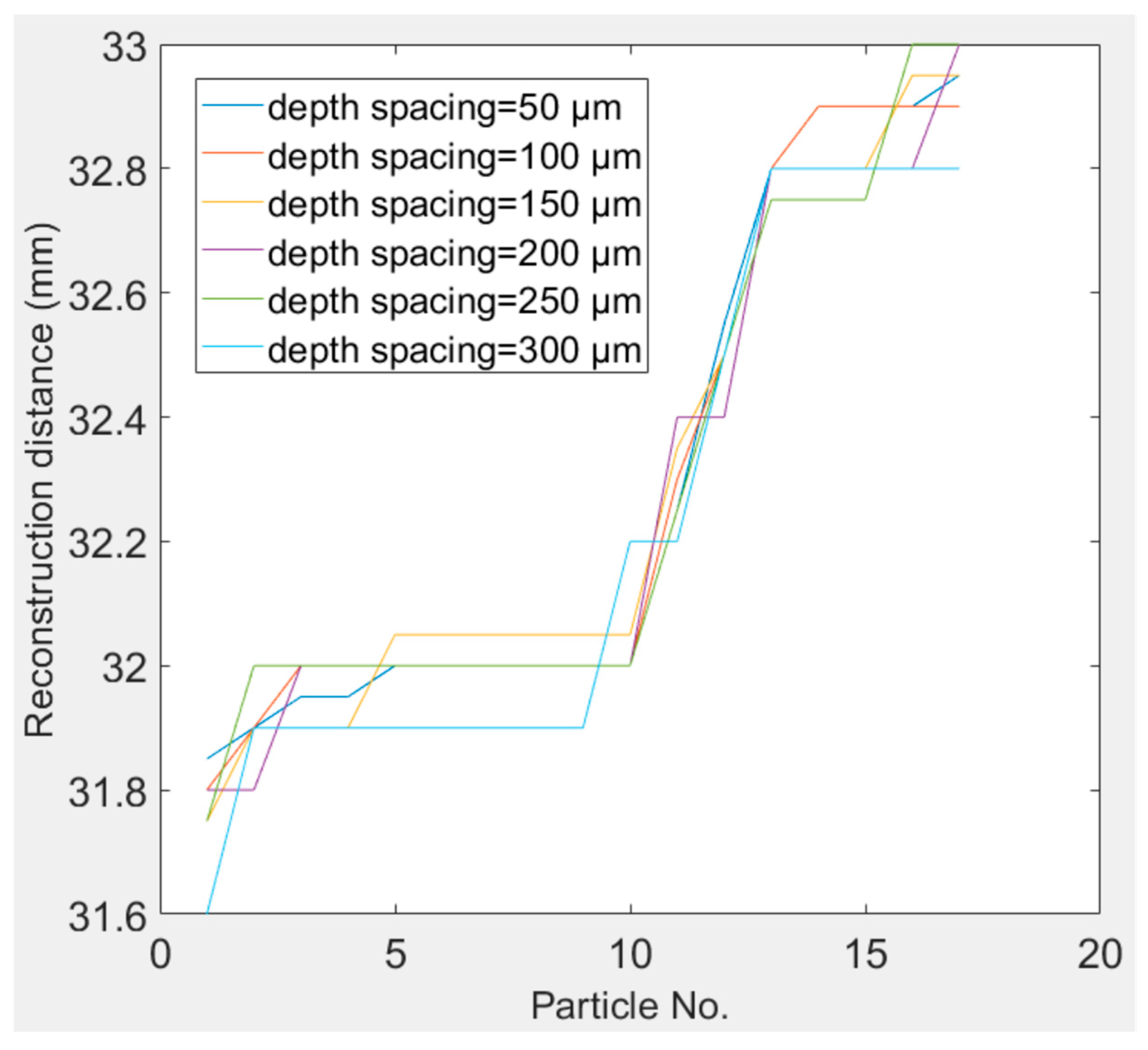
In this experiment, an in-line digital holographic experimental setup, as depicted in Figure 5a, was employed to capture the holograms. The used transparent particles were unibead monodispersed polystyrene microspheres, with diameters of 50 to 62 µm and solid content of 2.5% (w/v). First, a coherent (green) light source, with a wavelength of nm, was utilized to illuminate two layers of particles that were sandwiched between three glass slides; the thickness of each glass slide was about 1 mm. A hologram, which was captured by a CMOS camera with size and pixel pitch µm, is displayed in Figure 5b, and the synthetic minimum intensity image, which was the minimum value along the z-axis of all the raw reconstructed images generated in the distance range of (31, 34) mm with a depth spacing equal to 50 µm from this hologram, is shown in Figure 5c. There were a total of 17 particles in the two layers; the particles enclosed by the red circles were placed in one layer, whereas the particles enclosed by the green circles were placed in the other layer. The particle centroids, reim_index, and reconstruction distances are listed in Table 1. We obtained 17 particles when the depth spacing was equal to 50 µm (spent 29.0 s and generated 61 reconstructed images), 100 µm (spent 15.2 s and generated 31 reconstructed images), 150 µm (spent 10.5 s and generated 21 reconstructed images), 200 µm (spent 8.4 s and generated 16 reconstructed images), 250 µm (spent 6.9 s and generated 13 reconstructed images), and 300 µm (spent 6.2 s and generated 11 reconstructed images), respectively. The reconstruction distances of the particles corresponding to these reconstruction depth spacings are depicted in Figure 6. We can observe that these particles were relatively well distributed between the two slices.
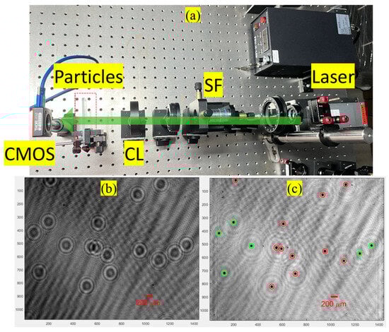
Figure 5.
(a) Experimental setup (SF: spatial filter; CL: collimating lens), (b) hologram (size ), and (c) synthetic minimum intensity image generated from all raw reconstructed images of hologram in (b).

Table 1.
Information for focused particles in Figure 5b’s hologram.
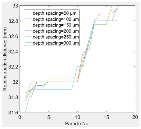
Figure 6.
Reconstruction distance of each particle corresponding to reconstruction depth spacings equal to 50 µm, 100 µm, 150 µm, 200 µm, 250 µm, and 300 µm, respectively.
4.2. Particles in Cuvette
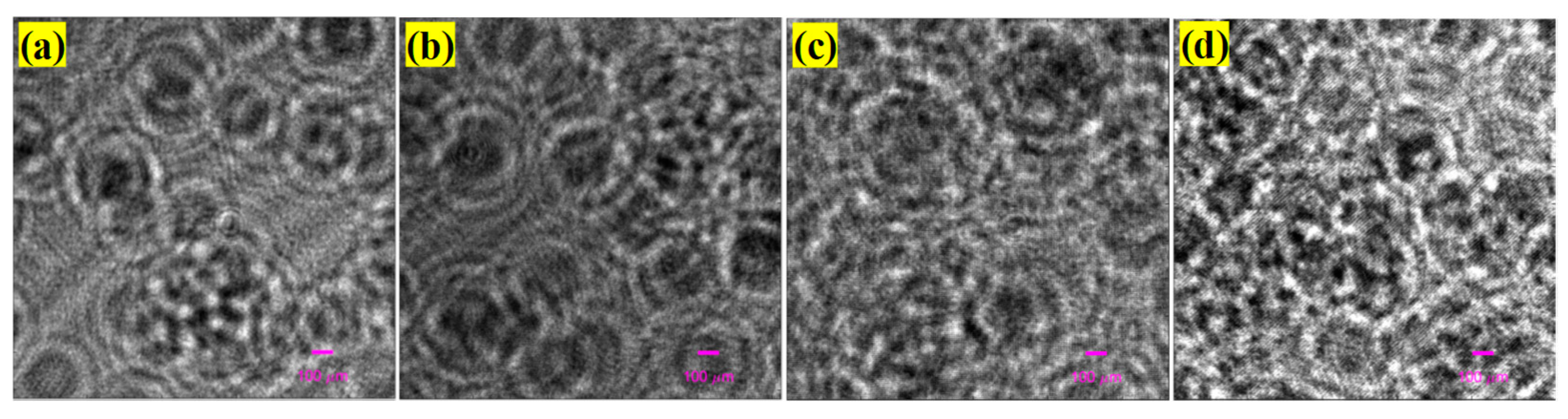
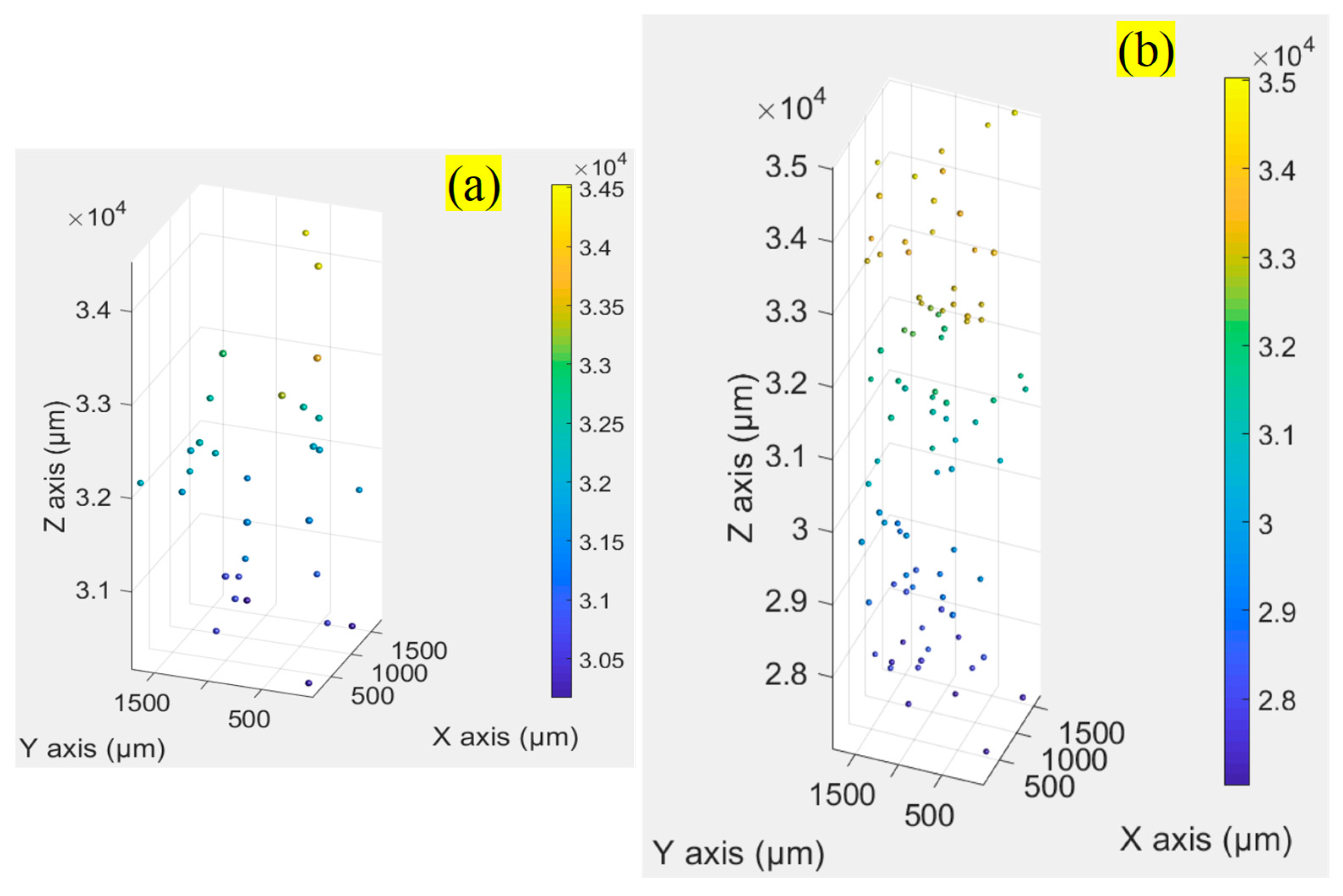
We continually captured holograms of large numbers of particles suspended in Milli-Q water that filled 3-mm (the dimension is mm3) and 10-mm (the dimension is mm3) cuvettes, respectively. In this section, only one particle solution, where approximately 3205 particles were seeded per mL, was made. We performed four experiments. In the first one, the 3-mm cuvette filled with the particle solution was placed 30 mm away from the same CMOS camera. While each captured original hologram was cropped into four equal smaller holograms (), so each smaller hologram captured a volume of mL. 16 holograms, each of which approximately contained 30 particles, were collected for this experiment. A hologram sample is shown in Figure 7a. We calculated the axial resolution at the distance of 30 mm to be approximately 2.5 mm, and the constrained intensity for each candidate focused particle must be less than 0.39, according to Section 3.2. Using the proposed method, we counted 498 focused particles from the 16 holograms and obtained a relative error of 3.75%. The particle distribution of the hologram from Figure 7a in 3D space is shown in Figure 8a.
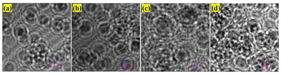
Figure 7.
Holograms (size ) of same particle solutions in (a) 3 mm cuvette placed at 30 mm away, (b) 3 mm cuvette placed at 40 mm away, (c) 3 mm cuvette placed at 60 mm away, and (d) 10 mm cuvette placed at 30 mm away from CMOS, respectively.

In the second experiment, we placed the same cuvette with the same particle solution 40 mm away from the CMOS camera. A total of 180 holograms with the size of , a hologram sample of which is shown in Figure 7b, were collected for this experiment. We calculated the axial resolution at the distance of 40 mm to be approximately 4.4 mm; however, because the thickness of the cuvette was only 3 mm, we still used the axial resolution of 2.5 mm instead of 4.4 mm, and the same constrained intensity for each candidate focused particle. Using the proposed method, we counted 5796 focused particles from the 180 holograms and obtained a relative error of 7.33%.
In the third experiment, we placed the same cuvette with the same particle solution 60 mm away from the CMOS camera. A total of 160 holograms with sizes of , a hologram sample of which is shown in Figure 7c, were collected for this experiment. We calculated the axial resolution at the distance of 60 mm to be approximately 9.8 mm; however, because the thickness of the cuvette was only 3 mm, we still used the axial resolution of 2.5 mm instead of 9.8 mm, and the same constrained intensity for each candidate focused particle. Using the proposed method, we counted 4841 focused particles from the 160 holograms and obtained a relative error of 0.85%.
In the last experiment, we used a 10 mm cuvette filled with the same particle solution and placed it at 30 mm away from the same CMOS camera. While the original captured holograms were cropped into four equal smaller holograms (), so each smaller hologram captured a volume of mL 200 holograms (), a hologram sample of which is displayed in Figure 7d, were collected for this experiment. Since the cuvette was placed 30 mm from the CMOS, we continually set the axial resolution to 2.5 mm and the constrained intensity to be the same as that in the previous experiments. We counted 18851 focused particles from the 200 holograms and obtained a relative error of 5.75%. The particle distribution of the hologram Figure 7d in 3D space is depicted in Figure 8b. The results of the four experiments are presented in detail in Table 2.
Table 2.
Detailed results of four experiments.
5. Conclusions
We propose an autofocusing method based on morphological analyses and axial resolution to obtain, relatively accurately, the 3D position of each particle, particularly its axial location, and the particle number of a dense transparent particle solution via a hologram. Our proposed method has two components. First, morphological analyses and constrained intensity are used on the raw reconstructed images, from which the information on candidate focused particles is then obtained and saved in one matrix. Second, axial resolution is utilized to obtain the real focused particles from the aforementioned matrix. For the focus metrics, we propose using the product of the mean intensity and equivalent diameter of each candidate focused particle. Eventually, we are able to secure all focused particles for one hologram. In our experiments, we used particles located at fixed distances and in a particle solution that was filled in a cuvette to examine and verify the proposed method. The deviations of the recognized axial locations were in the range of mm, and relative errors of the recognized particle numbers were less than 8%. Therefore, the proposed method is able to rapidly provide relatively accurate ground-truth axial positions for machine learning methods to solve the autofocusing problem that occurs with dense particles and makes it convenient to generate ground-truth datasets for these machine learning methods.
Author Contributions
Conceptualization, W.-N.L.; methodology, W.-N.L. and X.X.; validation, W.-N.L., Y.Z., J.C. and H.O.; formal analysis, X.X.; investigation, H.O.; data curation, W.-N.L.; writing—original draft preparation, W.-N.L.; writing—review and editing, W.-N.L., Y.Z., J.C., H.O. and X.X.; supervision, W.-N.L.; funding acquisition, W.-N.L. and X.X. All authors have read and agreed to the published version of the manuscript.
Funding
This study was supported by the STU Scientific Research Foundation for Talents and Guangdong University Key Platform [No. 2021GCZX009].
Data Availability Statement
Data underlying the results presented in this paper are not publicly available at this time but may be obtained from the authors upon reasonable request.
Conflicts of Interest
The authors declare no conflicts of interest.
References
- Garcla-Sucerqula, J.; Xu, W.; Jericho, S.K.; Klages, P.; Jericho, M.H.; Kreuzer, H.J. Digital in-line holographic microscopy. Appl. Opt. 2006, 45, 836–850. [Google Scholar] [CrossRef] [PubMed]
- Wu, Y.; Yao, L.; Brunel, M.; Coëtmellec, S.; Li, R.; Lebrun, D.; Zhou, H.; Gréhan, G.; Cen, K. Characterizations of transparent particle holography in near-field using Debye series. Appl. Opt. 2016, 55, A60–A70. [Google Scholar] [CrossRef] [PubMed]
- Gao, P.; Yao, B.; Min, J.; Guo, R.; Ma, B.; Zheng, J.; Lei, M.; Yan, S.; Dan, D.; Ye, T. Autofocusing of digital holographic microscopy based on off-axis illuminations. Opt. Lett. 2012, 37, 3630–3632. [Google Scholar] [CrossRef] [PubMed]
- Zheng, J.; Gao, P.; Shao, X. Opposite-view digital holographic microscopy with autofocusing capability. Sci. Rep. 2017, 7, 4255. [Google Scholar] [CrossRef]
- Langehanenberg, P.; von Bally, G.; Kemper, B. Autofocusing in digital holographic microscopy. 3D Res. 2011, 2, 4. [Google Scholar] [CrossRef]
- Ilhan, H.A.; Doğar, M.; Özcan, M. Digital holographic microscopy and focusing methods based on image sharpness. J. Microsc. 2014, 255, 138–149. [Google Scholar] [CrossRef]
- Ren, Z.; Chen, N.; Lam, E.Y. Automatic focusing for multisectional objects in digital holography using the structure tensor. Opt. Lett. 2017, 42, 1720–1723. [Google Scholar] [CrossRef]
- Zhang, Y.; Wang, H.; Wu, Y.; Tamamitsu, M.; Ozcan, A. Edge sparsity criterion for robust holographic autofocusing. Opt. Lett. 2017, 42, 3824–3827. [Google Scholar] [CrossRef]
- Lyu, M.; Yuan, C.; Li, D.; Situ, G. Fast autofocusing in digital holography using the magnitude differential. Appl. Opt. 2017, 56, F152–F157. [Google Scholar] [CrossRef]
- Khanam, T.; Darakis, E.; Rajendran, A.; Kariwala, V.; Asundi, A.K.; Naughton, T.J. On-line digital holographic measurement of size and shape of microparticles for crystallization processes. Proc. SPIE 2008, 7155, 514–523. [Google Scholar]
- Darakis, E.; Khanam, T.; Rajendran, A.; Kariwala, V.; Naughton, T.J.; Asundi, A.K. Microparticle characterization using digital holography. Chem. Eng. Sci. 2010, 65, 1037–1044. [Google Scholar] [CrossRef]
- Kempkes, M.; Darakis, E.; Khanam, T.; Rajendran, A.; Kariwala, V.; Mazzotti, M.; Naughton, T.J.; Asundi, A.K. Three dimensional digital holographic profiling of micro-fibers. Opt. Express 2009, 17, 2938–2943. [Google Scholar] [CrossRef]
- Khanam, T.; Rajendran, A.; Kariwala, V.; Asundi, A.K. Measurement of two-dimensional crystal shape using digital holography. Cryst. Growth Des. 2013, 13, 3969–3975. [Google Scholar] [CrossRef]
- Tian, L.; Loomis, N.; Domínguez-Caballero, J.A.; Barbastathis, G. Quantitative measurement of size and three-dimensional position of fast-moving bubbles in air-water mixture flows using digital holography. Appl. Opt. 2010, 49, 1549–1554. [Google Scholar] [CrossRef] [PubMed]
- Lang, K.; Qiang, J.; Qiu, Y.; Wang, X. Autofocusing method for multifocal holograms based on connected domain analysis. Opt. Lasers Eng. 2025, 184, 108624. [Google Scholar] [CrossRef]
- Brady, D.J.; Choi, K.; Marks, D.L.; Horisaki, R.; Lim, S. Compressive holography. Opt. Express 2009, 17, 13040–13049. [Google Scholar] [CrossRef]
- Liu, Y.; Tian, L.; Lee, J.W.; Huang, H.Y.H.; Triantafyllou, M.S.; Barbastathis, G. Scanning-free compressive holography for object localization with subpixel accuracy. Opt. Lett. 2012, 37, 3357–3359. [Google Scholar] [CrossRef]
- Liu, Y.; Tian, L.; Hsieh, C.-H.; Barbastathis, G. Compressive holographic two-dimensional localization with 1/302 subpixel accuracy. Opt. Express 2014, 22, 9774–9782. [Google Scholar] [CrossRef]
- Chen, W.; Tian, L.; Rehman, S.; Zhang, Z.; Lee, H.P.; Barbastathis, G. Empirical concentration bounds for compressive holographic bubble imaging based on a Mie scattering model. Opt. Express 2015, 23, 4715–4725. [Google Scholar] [CrossRef]
- Li, W.-N.; Zhang, Z.; Su, P.; Ma, J.; Wang, X. Removal of defocused images using three- -dimensional nonlinear diffusion based on digital holography. J. Opt. 2020, 22, 051701. [Google Scholar] [CrossRef]
- Ren, Z.; Xu, Z.; Lam, E.Y. Learning-based nonparametric autofocusing for digital holography. Optica 2018, 5, 337–344. [Google Scholar] [CrossRef]
- Lee, S.J.; Yoon, G.Y.; Go, T. Deep learning-based accurate and rapid tracking of 3D positional information of microparticles using digital holographic microscopy. Exp. Fluids 2019, 60, 170. [Google Scholar] [CrossRef]
- Shao, S.; Mallery, K.; Hong, J. Machine learning holography for measuring 3D particle distribution. Chem. Eng. Sci. 2020, 225, 115830. [Google Scholar] [CrossRef]
- Wu, Y.; Wu, J.; Jin, S.; Cao, L.; Jin, G. Dense-U-net: Dense encoder-decoder network for holographic imaging of 3D particle fields. Opt. Commun. 2021, 493, 126970. [Google Scholar] [CrossRef]
- Li, W.-N.; Su, P.; Ma, J.; Wang, X. Short U-net model with average pooling based on in-line digital holography for simultaneous restoration of multiple particles. Opt. Lasers Eng. 2021, 139, 106449. [Google Scholar] [CrossRef]
- Hao, Z.; Li, W.-N.; Hou, B.; Su, P.; Ma, J. Characterization method for particle extraction from raw-reconstructed images using U-net. Front. Phys. 2022, 9, 816158. [Google Scholar] [CrossRef]
- Ou, H.; Lin, W.; Li, W.-N.; Xie, X. Real-time particle concentration measurement from a hologram by deep learning. Phys. Scr. 2024, 99, 095512. [Google Scholar] [CrossRef]
- Goodman, J.W. Introduction to Fourier Optics, 4th ed.; W. H. Freeman: New York, NY, USA, 2017. [Google Scholar]
- Born, M.; Wolf, E. Principles of Optics, 7th ed.; Cambridge University Press: Cambridge, UK, 1999. [Google Scholar]
- Meng, H.; Hussain, F. In-line recording and off-axis viewing technique for holographic particle velocimetry. Appl. Opt. 1995, 34, 1827–1840. [Google Scholar] [CrossRef]
- Li, H.; Ji, F.; Li, L.; Li, B.; Ma, F. In lab in-line digital holography for cloud particle measurement experiment. Proc. SPIE 2016, 10156, 1015618. [Google Scholar]
Disclaimer/Publisher’s Note: The statements, opinions and data contained in all publications are solely those of the individual author(s) and contributor(s) and not of MDPI and/or the editor(s). MDPI and/or the editor(s) disclaim responsibility for any injury to people or property resulting from any ideas, methods, instructions or products referred to in the content. |
© 2025 by the authors. Licensee MDPI, Basel, Switzerland. This article is an open access article distributed under the terms and conditions of the Creative Commons Attribution (CC BY) license (https://creativecommons.org/licenses/by/4.0/).