In this section, we apply the proposed technique to several analytic and simulated examples when the time delay is either known exactly or can be estimated using other techniques. We also consider the effect of noise presence on the accuracy of time delay estimation.
5.1. Four-Pole Example
Consider a transfer function with four poles and time delay
, defined by:
with:
where
,
,
,
, and
. Since the poles of
are located in the upper half
w-plane at
and
, this function is causal as a sum of four causal transforms and has no time delay. Therefore, the function
is a causal function delayed with offset
.
H is sampled on
at
N frequency points varying from
to 1500 with
.
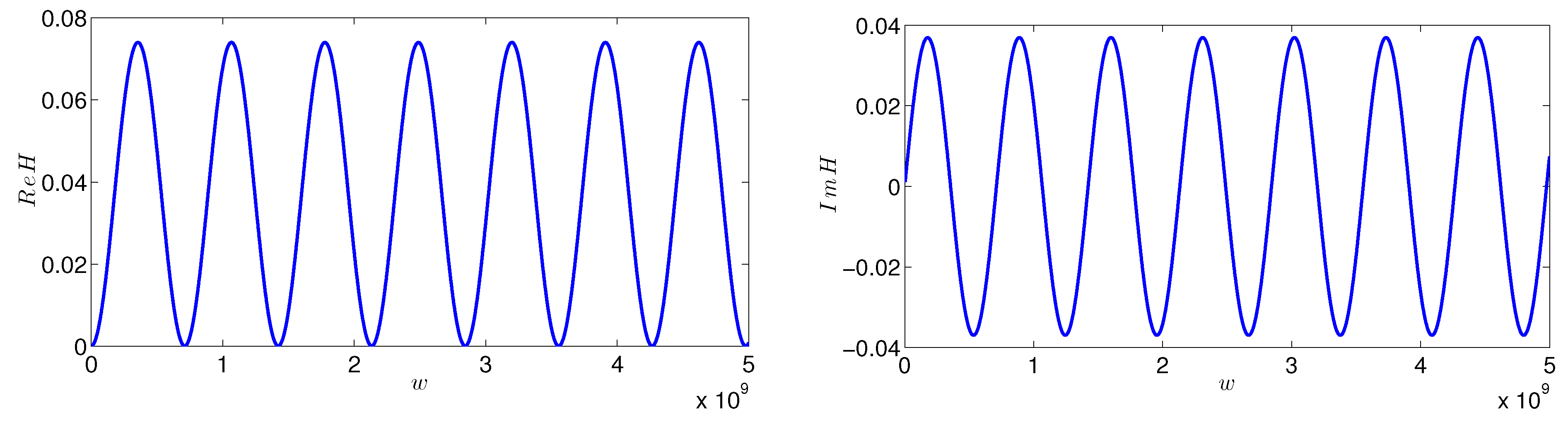
The real and imaginary parts of
are shown in
Figure 1. After rescaling with
and reflecting to negative frequencies, we obtain a rescaled transfer function
defined on
, for which we construct a causal Fourier continuation
defined in Equation (
9) using
Fourier coefficients. Hence, the number
M of Fourier coefficients also varies between 50 and 1500.
and
of the rescaled and reflected
together with their causal Fourier continuations with
are depicted in
Figure 2. Even though given
and its causal Fourier continuation approximation look indistinguishable, the actual reconstruction errors
and
in both the real and imaginary parts, which are defined in (13) and (14), are on the order of
, and they decrease as
M increases (with
). For example, with
, the errors are on the order of
. Since both errors
and
are of the same order, it is enough to analyze one of the errors, for example
. The results using
are similar.
Figure 1.
and in the four-pole example.
Figure 1.
and in the four-pole example.
Figure 2.
and of the rescaled and reflected by symmetry transfer function in the four-pole example together with their causal Fourier continuations and , respectively, with Fourier coefficients.
Figure 2.
and of the rescaled and reflected by symmetry transfer function in the four-pole example together with their causal Fourier continuations and , respectively, with Fourier coefficients.
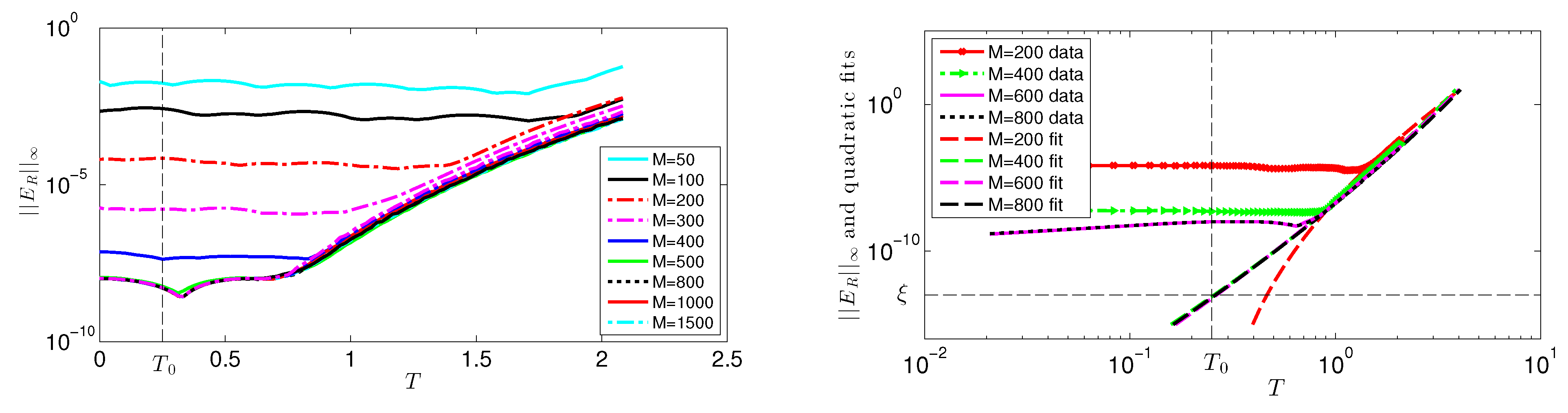
To estimate the time delay, we analyze the evolution of
, the
∞ norm of
, shown in
Figure 3, for various values
M.
Figure 3.
Evolution of the reconstruction error as a function of T in the four-pole example. The dashed line corresponds to the exact delay .
Figure 3.
Evolution of the reconstruction error as a function of T in the four-pole example. The dashed line corresponds to the exact delay .
Since the error due to a causal Fourier series approximation decreases with
M (see error bound (16)), the reconstruction error between the given transfer function
H and its causal Fourier continuation
also decreases as
M increases until it either reaches the level
ξ of filtering of singular values or a level
ϵ of noise/causality violations (see error bounds (17) and (18), respectively). For each fixed
M, as time
T increases, the errors
and
first are small and about of the same order until some transition time close to the time delay
is approached. After that, the errors grow approximately as a power function on the log-log scale. For smaller
T, the errors are dominated by a causal Fourier series approximation error. Then for
T greater than some transition time, they are dominated by causality violations since this value
T provides a large enough negative time delay and shifts a causal function into a non-causal area. A transition value
, we call it a critical time, from a plateau region to a growth region is different for each
M. It decreases as the resolution or number of Fourier coefficients increases if the error is dominated by the causal Fourier series approximation error. The critical times
approach the time delay
as
M increases. The goal is to estimate
using the error curves shown in
Figure 3. Analyzing graphs of the error curves for
, we observe some non-monotonic behavior at
T close to
. This behavior is due to the filtering of the singular values below the threshold
that we used in our experiments. By increasing the value of
ξ, the non-monotonic behavior will be present at smaller values of
M. This suggests that portions of error curves close to threshold
ξ are affected by filtering and may be inaccurate and difficult to use for time delay estimation as we find in our experiments. To estimate critical times
of transition from the plateau region to the growth region, we approximate the growing region by a quadratic function on the log-log scale. Specifically, we assume that
, where coefficients
,
and
are determined in the least squares sense. The resulting quadratic function
is then evaluated at the value of
at
that is assumed to be the “most causal” time. By taking the exponential function of the result, we find a critical transition time
for a given
M. This procedure produces estimates of the time delay
for various values of
M. The graph of the critical transition times
as a function of
M is shown in
Figure 4. One can clearly see that the critical times approach the exact time delay
as
M increases. A good approximation of
is achieved at
.
Figure 4.
Critical transition times in the four-pole example that approach as M increases. The dashed line corresponds to the exact delay .
Figure 4.
Critical transition times in the four-pole example that approach as M increases. The dashed line corresponds to the exact delay .
The values of
for
are presented in
Table 1. The results indicate that the approximations become more accurate as
M increases. The error with
is less than 1%. At the same time, the error with
is about 3%, which is due to the fact that the results in this case are more affected by the filtering of singular values. In the cases when
M is high and the resulting error is not flat for
, instead of evaluating a fitted quadratic curve at the value of
at
, we evaluate it at
ξ, the threshold of filtering singular values, to avoid using results affected by filtering.
Table 1.
Critical transition times in the four-pole example that approach as M increases.
Table 1.
Critical transition times in the four-pole example that approach as M increases.
| M | | M | |
|---|
| 200 | 1.4604 | 700 | 0.3394 |
| 300 | 1.1294 | 800 | 0.2529 |
| 400 | 0.9077 | 900 | 0.2497 |
| 500 | 0.6655 | 1000 | 0.2472 |
| 600 | 0.4759 | 1500 | 0.2576 |
In practice, the number
N of samples of the transfer function
is usually limited, which sets the bound for the number
of Fourier coefficients, so it may not always be possible to use large enough
M to obtain critical time
close enough to the actual time delay
. A good method should be capable of producing an accurate approximation of
even with a small number of data points. We achieve this by employing another approach for time delay estimation. Using the obtained fitted quadratic error curves, we extrapolate them to the value
ξ of the filtering of singular values, which is typically chosen to be close to the machine precision. This corresponds to finding time
T at which the error reaches the value
ξ. This choice is natural, since the errors below
ξ are most likely affected by filtering and may not be accurate enough to use. The results of such extrapolation are shown in
Figure 5 for
, 400, 600 and 800. An intersection of the extrapolated curve corresponding to
is at a value
, which is a bit far from the exact
. At the same time, intersections of extrapolated curves with higher values of
M are much closer; see
Table 2 for details.
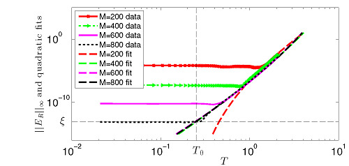
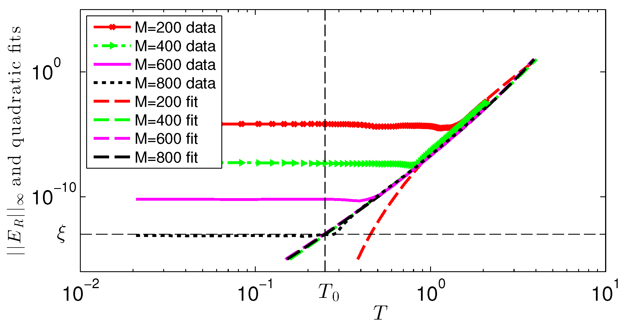
Figure 5.
in the four-pole example with , 400, 600 and 800 together with their extrapolated quadratic fits. The vertical dashed line indicates the exact time delay , while the horizontal dashed line indicates the level of filtering of singular values given by .
Figure 5.
in the four-pole example with , 400, 600 and 800 together with their extrapolated quadratic fits. The vertical dashed line indicates the exact time delay , while the horizontal dashed line indicates the level of filtering of singular values given by .
Table 2.
Approximations of in the four-pole example using extrapolation. The exact value , averaged value .
Table 2.
Approximations of in the four-pole example using extrapolation. The exact value , averaged value .
| M | Approximation | M | Approximation |
|---|
| 200 | 0.45451 | 700 | 0.24734 |
| 300 | 0.27235 | 800 | 0.24969 |
| 400 | 0.25297 | 900 | 0.24974 |
| 500 | 0.25053 | 1000 | 0.24724 |
| 600 | 0.24633 | 1500 | 0.25759 |
Results shown in
Table 2 indicate that as
M increases, the extrapolated quadratic curve intersects the horizontal line with the value
ξ at times closer to
. Obtained approximations of
can be averaged producing
. The approach with extrapolation provides a faster convergence and good approximations of
even for small values of
M,
i.e., less data points are needed to approximate
.
We also consider the effect of noise on the time delay estimation. To study this, we impose a sine perturbation:
of various amplitudes
a that we add to
, while keeping
unchanged. We choose
and vary
a from
–
. For the convenience of the reader, the perturbed profiles of
are shown in the left panel of
Figure 6 using the signal-to-noise ratio (SNR) format, where we consider ratios of
to the amplitude
a of the perturbation, presenting them in dB units,
i.e., plotting
. The reconstruction error
with no perturbation for early times
is of the order of
, as shown in the right panel of
Figure 6, that corresponds to the level of the filtering of singular values. When the perturbation is added, the reconstruction errors for
are higher and approximately of the order of
a. Once some critical transition time greater than
is passed, reconstruction errors start growing. They grow at the same rate and coincide almost perfectly with each other. This observation suggests that the proposed approach can also be used in the cases when data have a noise, which is typical in real-life applications, when data have either measurement or simulation errors. For noise with a smaller amplitude, the region close to
will be less affected by noise, and a bigger growing region will be available for fitting, so we expect better accuracy of time delay estimation in such cases. When more noise in data is present, the less growing region will be available for fitting, and the extrapolation of fitted quadratic error curves may be less accurate. We demonstrate this by considering two cases: with
(noisier case) and
(less noisy case).
Figure 6.
Left panel: profiles of perturbed in the signal-to-noise ratio (SNR) format, i.e., , plotted in dB. Right panel: evolution of in the four-pole example with added sine perturbation . The vertical dashed line corresponds to the exact delay .
Figure 6.
Left panel: profiles of perturbed in the signal-to-noise ratio (SNR) format, i.e., , plotted in dB. Right panel: evolution of in the four-pole example with added sine perturbation . The vertical dashed line corresponds to the exact delay .
Figure 7.
Left panel: evolution of in the four-pole example with the added perturbation . The dashed line corresponds to the exact delay . Right panel: error curves in the four-pole example with the added perturbation and , 400, 600 and 800 together with their extrapolated quadratic fits. The vertical dashed line indicates the exact time delay , while the horizontal dashed line indicates the level of filtering of singular values given by .
The error curves with a higher amplitude
are presented in the left panel of
Figure 7. It is clear that the error does not become smaller than
as
gets larger because of the noise. We use available growing regions and extrapolate fitted error curves to find their intersection with the horizontal line with value
ξ. This gives us time
T when the error reaches the value
ξ for each considered
M. The results of such extrapolation for
, 400, 600 and 800 are shown in the right panel of
Figure 7. Clearly, extrapolated error curves reach value
ξ at times around
, but not close enough to
and without established convergence, but rather in a spread-out manner around
.
Approximations of
for the values of
M that we investigated are shown in
Table 3. Averaging these approximations, we obtain
. The extrapolated curves can be made more focused around
by narrowing down the fitted region. The results of this procedure are shown in
Figure 8. This improves the average time delay to
.
Table 3.
Approximations of in the four-pole example with perturbation using extrapolations with original fitting regions for various M. The exact value , averaged value .
Table 3.
Approximations of in the four-pole example with perturbation using extrapolations with original fitting regions for various M. The exact value , averaged value .
| M | Approximation | M | Approximation |
|---|
| 200 | 0.40158 | 700 | 0.39113 |
| 300 | 0.25578 | 800 | 0.28392 |
| 400 | 0.19863 | 900 | 0.26543 |
| 500 | 0.14311 | 1000 | 0.20293 |
| 600 | 0.45358 | 1500 | 0.32837 |
Figure 8.
in the four-pole example with the added perturbation and , 400, 600 and 800 together with their extrapolated quadratic fits constructed using more narrow fitting region. The vertical dashed line indicates the exact time delay = , while the horizontal dashed line indicates the level of filtering of singular values given by ξ = .
Next, we show the results when a smaller noise of amplitude
is added. The evolution of
as
T increases is shown in the left panel of
Figure 9. We can see that the plateau error region in this case is at about the
level, so the error growth region is bigger than in the previous case, which should make fitting and extrapolation more accurate.
Indeed, extrapolated quadratic curves intersect the horizontal line with value
ξ in a more localized region about
, as shown in the right panel of
Figure 9, while averaging of obtained approximations to
produces
, which is more accurate than in the case with a higher amplitude
. Approximations of
for various
M are shown in
Table 4.
Figure 9.
Left panel: evolution of in the four-pole example with the added perturbation of a smaller amplitude. The dashed line corresponds to the exact delay . Right panel: in the four-pole example with the added perturbation and , 400, 600 and 800 together with their extrapolated quadratic fits. The vertical dashed line indicates the exact time delay , while the horizontal dashed line indicates the level of filtering of singular values given by .
Table 4.
Approximations of in the four-pole example with perturbation using extrapolations for various M. The exact value , averaged value = .
Table 4.
Approximations of in the four-pole example with perturbation using extrapolations for various M. The exact value , averaged value = .
| M | Approximation | M | Approximation |
|---|
| 200 | 0.46392 | 700 | 0.25502 |
| 300 | 0.27635 | 800 | 0.26081 |
| 400 | 0.25683 | 900 | 0.2444 |
| 500 | 0.26798 | 1000 | 0.25582 |
| 600 | 0.26391 | 1500 | 0.25292 |
5.2. Transmission Line Example
We consider a uniform transmission line segment with the following per unit-length parameters:
L =
nH/inches,
pF/inches,
/inches,
μS/inches and length
inches. The frequency is sampled on the interval
GHz. The scattering matrix of the structure is computed using MATLAB function
rlgc2s. We consider the element
and impose the time delay
ns by multiplying
by
to get the delayed transfer function
. The real and imaginary parts of
are given in
Figure 10.
Figure 10.
and in the transmission line example.
Figure 10.
and in the transmission line example.
The error curves for different
M are shown in the left panel of
Figure 11, indicating that the reconstruction error decreases quickly as
M increases and reaches the level close to machine precision at
.
Figure 11.
Left panel: evolution of in the transmission line example as M varies. The vertical dashed line indicates the time delay ns. Right panel: estimation of the delay time in the transmission line example using critical transition times as M varies. The dashed line corresponds to the exact delay ns.
Figure 12.
in the transmission line example with , 400, 600 and 800 together with their quadratic fits. The vertical dashed line indicates the exact time delay = ns, while the horizontal dashed line indicates the level of filtering of singular values given by .
Figure 12.
in the transmission line example with , 400, 600 and 800 together with their quadratic fits. The vertical dashed line indicates the exact time delay = ns, while the horizontal dashed line indicates the level of filtering of singular values given by .
Constructing fitted quadratic error curves and finding their intersections with
at
or finding times when these fitted error curves reach the value
ξ of the error for
, we get a sequence of critical transition times
, which we show in the right panel of
Figure 11. Clearly, critical times
converge to
and provide a good approximation of
for
. Using an alternative approach when we extrapolate the fitted quadratic error curves to find their intersections with the error threshold
ξ, we also obtain good approximations of
. Some of these curves for
, 400, 600 and 800 are depicted in
Figure 12.
Approximations of
using the extrapolation procedure for various values of
M ranging from
M = 200 to 1500 are given in
Table 5. An accurate approximation of
is obtained even with
. As before, approximations of
become better as
M increases, but for very large values of
when the reconstruction error falls below the filtering threshold
ξ and filtering affects the results more, extrapolation becomes less accurate. Averaging obtained approximations of
produces
ns, which is very close to the exact value
ns.
Table 5.
Approximations of (in ns) in the transmission line example using extrapolations for various M. The exact value ns, averaged value ns.
Table 5.
Approximations of (in ns) in the transmission line example using extrapolations for various M. The exact value ns, averaged value ns.
| M | Approximation | M | Approximation |
|---|
| 200 | | 700 | |
| 300 | | 800 | |
| 400 | | 900 | |
| 500 | | 1000 | |
| 600 | | 1500 | |
5.4. Stripline Example
We simulated an asymmetric stripline modeled in [
39] with length
in, width
mils, distances from the trace to reference planes
mils,
mils, substrate dielectric Megtron6-1035, laminate with a dielectric constant
using a Cadence software tool with an FEM full-wave field solver. The scattering matrix
S is obtained on
with
GHz. We analyze element
of the transfer matrix. The real and imaginary parts of
H are shown in
Figure 15.
Figure 15.
and in the stripline example with .
Figure 15.
and in the stripline example with .
The evolution of
for various
M is depicted in
Figure 16. Even for high values of
M, the error in causality does not go to the machine precision or the filtering level
ξ and, instead, levels off around
. This indicates that our finite element simulation results are accurate only within
. For causality characterization, this implies that data have noise/approximation errors with an amplitude around
. Graphs of
suggest that for
, the error is dominated by Fourier series approximation error, while for higher
M, the error is dominated by the noise/approximation errors from the finite element method.
Figure 16.
in the stripline example for various M. The vertical dashed line indicates the closed form microwave theory time delay approximation ns.
Figure 16.
in the stripline example for various M. The vertical dashed line indicates the closed form microwave theory time delay approximation ns.
In this example, the time delay is estimated using a closed form microwave theory approximation as
ns, where
m/s is the speed of light and
is a conversion factor to convert from inches to meters. The error curves were fitted to quadratic curves, as explained above. Because of the relatively high errors in the data, the fitted regions are not long enough. Besides, there is more nonlinear behavior of the error curves for high values of
. All this makes it difficult to estimate the time delay, as shown in the left panel of
Figure 17. As can be seen, extrapolated quadratic curves do not focus at
, but instead spread out around
, similarly to the four-pole example with an imposed noise of relatively large amplitude considered in
Section 5.1.
Figure 17.
Left panel: extrapolated quadratic curves based on the initial fitting range in the stripline example. Right panel: extrapolated quadratic curves based on a more narrow fitting range in the stripline example. The average time delay is ns.
Figure 17.
Left panel: extrapolated quadratic curves based on the initial fitting range in the stripline example. Right panel: extrapolated quadratic curves based on a more narrow fitting range in the stripline example. The average time delay is ns.
This problem can be corrected by decreasing the fitting range and going further away from transition regions. The results are shown in the right panel of
Figure 17.
The approximations of
are given in
Table 7. Averaging them for values of
M up to 3000 produces
ns, which agrees well with an analytically estimated time delay using a closed form formula. As in other examples, results with very high values of
, which are more affected by noise and approximation errors in data, are less accurate.
Table 7.
Approximations of (in ns) in the stripline example using extrapolations of fitted quadratic error curves for various M. The closed form approximation of the time delay is ns, and the averaged value is ns for M ranging up to 3000.
Table 7.
Approximations of (in ns) in the stripline example using extrapolations of fitted quadratic error curves for various M. The closed form approximation of the time delay is ns, and the averaged value is ns for M ranging up to 3000.
| M | Approximation | M | Approximation |
|---|
| 80 | 1.266 | 700 | 1.1987 |
| 100 | 1.2312 | 800 | 1.2179 |
| 200 | 1.2553 | 900 | 1.2593 |
| 300 | 1.2797 | 1000 | 1.2205 |
| 400 | 1.2826 | 2000 | 1.246 |
| 500 | 1.2413 | 3000 | 1.5878 |
| 600 | 1.1833 | 4000 | 1.0168 |
5.5. Finite Element Model of a DDR4 Module with a DRAM Package
In this example, we use a scattering matrix
S generated by a finite element modeling of a DDR4 module with a DRAM package (courtesy of Micron Technology, Inc.). The package is attached to the module using ball grid array (BGA) technology. The model includes a no-die DRAM package on a printed circuit board (PCB). The model contains 110 input and output ports. The simulation process is performed for 100 equally spaced frequency points ranging from
=0 to
GHz using ANSYS Electromagnetics Suite. For time delay analysis, we consider a group of address buses A8–A4 from module pins to package die-side pins. The port assignment for this group is as follows. Port 1 is placed at the junction of the package and PCB or the BGA; Port 2 is placed at the die-side pin of the package; and Port 3 is placed at the module pin. Hence,
represents how the signal is transmitted on the address bus from the BGA to the die;
shows how the signal is transmitted from the BGA to the module pin; while
represents how the signal is transmitted from the die to the module pin. The magnitudes of these scattering parameters in a signal-to-noise ratio format are shown in
Figure 18 assuming that the data accuracy is
, as justified below.
We chose the element
to test the performance of the proposed method. The real and imaginary parts of
H are shown in
Figure 19. Since the number
of data points is fixed in this example, we first use
Fourier coefficients. The evolution of
reveals that the causality for early times is satisfied only within
, suggesting either low data resolution or relatively high approximation errors in the data. Approximating the time delay
by extrapolating only one error curve to the filtering threshold
may be inaccurate, so we decided to construct causal Fourier series approximations for several numbers
M of Fourier coefficients ranging from
to 600 while keeping the same resolution with
to get several approximations of the time delay
. Using more than
Fourier coefficients did not significantly affect the causality accuracy, as can be seen in the left panel of
Figure 20. The results indicate that the data are only accurate within
at most, which is consistent with the expected accuracy of the finite element simulations of the model. It should be noted that with
, causal Fourier series approximations become more oscillatory, and the amplitude of the oscillations increases as
M increases. In fact, for
, we construct trigonometric interpolants with very small errors at collocation data points, but large oscillations between the collocation points. The presence of such spurious oscillations is the reason why over-collocation [
38] is suggested for SVD-based Fourier continuations. With over-collocation, the number of data points should exceed the number of Fourier coefficients, and it is recommended to use at least twice more collocation data points than the number
M of Fourier coefficients. We have
data points because of the spectrum symmetry, and we use
Fourier coefficients to get accurate and non-oscillatory causal Fourier series approximations. Even though using more Fourier coefficients
M in this example than the number
N of collocation points affected causal Fourier series approximations, the qualitative dynamics of the error curves has not changed. At the same time, having several error curves that can be extrapolated to the level
ξ provided several approximations of the time delay
, which we can use to get an average time delay.
Figure 18.
Magnitudes of elements , and in dB using the signal-to-noise ratio (SNR) format in the DDR4 module with a DRAM package example with data accuracy.
Figure 18.
Magnitudes of elements , and in dB using the signal-to-noise ratio (SNR) format in the DDR4 module with a DRAM package example with data accuracy.
Figure 19.
and of the element from the DDR4 module with a DRAM package example.
Figure 19.
and of the element from the DDR4 module with a DRAM package example.
In the right panel of
Figure 20, we show several error curves together with their extrapolated quadratic fits. The fits were obtained using a more localized fitting range, since the data have a relatively high level of error.
Figure 20.
Left panel: evolution of for various M in the DDR4 module with a DRAM package example. The vertical dashed line indicates the time delay ns estimated using alternative methods. Right panel: error curves together with their extrapolated quadratic curves, and the horizontal dashed line indicates the level of filtering of singular values given by . The average time delay is ns.
The approximation of the time delay
using various values of
M is shown in
Table 8. Averaging them, we obtain
ns.
Table 8.
Approximations of (in ns) in the DDR4 module with a DRAM package example using extrapolations of fitted quadratic error curves for various M. An estimate of the time delay obtained using alternative methods is ns. The average time delay obtained using various numbers of Fourier coefficients ranging from 100 to 600 is ns.
| M | Approximation | M | Approximation |
|---|
| 100 | | 240 | |
| 150 | | 300 | |
| 170 | | 400 | |
| 180 | | 500 | |
| 200 | | 600 | |
For comparison, the time delay
is estimated using two other alternative methods. In the first method, since
S parameters have units of voltage amplitudes,
is considered as a minimum-phase transfer function [
26]. The plot of the phase of
, shown in the left panel of
Figure 21, reveals that the phase of
is approximately a linear function for the frequencies we consider (for higher frequencies, it is expected to have a more nonlinear behavior). Its slope can be used to approximate the time delay. For example, from DC to 3.939 GHz, the phase of
has changed −0.9996 radians. This implies that the time delay
ns. Alternatively, the slope of the phase of
can be approximated by using the linear least squares fitting. We find the slope to be
. Dividing it by
gives
ns.
Another way to estimate the time delay from
S-parameters is by using the time domain transmission (TDT). The input step function is initialized with the sample time
ps and rise time
ps, and it is shown in the right panel of
Figure 21 using a solid blue line. The transfer function
is fit to a rational function using the vector fitting method implemented in the MATLAB function
rationalfit. Since the bandwidth of
is only 5 GHz and the transfer function does not decay enough, we extend the bandwidth of the fitted rational function to 50 GHz to avoid aliasing according to the Nyquist criterion. Then, we use the inverse fast Fourier transform to compute the response of the system to the unit step function due to
in the time domain. This response is shown in the right panel of
Figure 21 using a dashed red line. Measuring times at which the input step function and the output step response reach
of their maximum values and taking their difference, we obtain an approximation to the time delay
.
The average time delay ns obtained using the proposed method is consistent with other alternative approximations of the time delay, which demonstrates the robustness of our technique.
Figure 21.
Left panel: phase of as a function of frequency in the DDR4 module with a DRAM package example. Its slope is , which gives an approximation of the time delay ns.
Figure 21.
Left panel: phase of as a function of frequency in the DDR4 module with a DRAM package example. Its slope is , which gives an approximation of the time delay ns.


