Article

Nonlinearities Associated with Impaired Sensors in a Typical SHM Experimental Set-Up

Department of Innovation Engineering, University of Salento, 73100 Lecce, Italy
*
Author to whom correspondence should be addressed.
Electronics 2018, 7(11), 303; https://doi.org/10.3390/electronics7110303
Submission received: 16 October 2018 / Revised: 1 November 2018 / Accepted: 5 November 2018 / Published: 6 November 2018
(This article belongs to the Special Issue Sensing and Signal Processing in Smart Healthcare)

Abstract

:
Structural Health Monitoring (SHM) gives a diagnosis of a structure assessing the structural integrity and predicting the residual life through appropriate data processing and interpretation. A structure must remain in the design domain, although it can be subjected to normal aging due to usage, action of the environment, and accidental events. SHM involves the integration of electronic devices in the inspected structure that sometimes are Piezoelectric Transducers (PZT). These are lightweight and small and can be produced in different geometries. They are used both in guided wave-based and electromechanical impedance-based methods. The PZT bonding requires essential steps such as preparation of the surfaces, application of the adhesive, and assembly that make the bonding process not so easy to be realised. Furthermore, adhesives are susceptible to environmental degradation. Transducer debonding or non-uniform distributed glue underneath the sensor causes the reduction of the performance and can affect the reliability of the SHM system. In this paper, a sensor diagnostic method for the monitoring of the PZT operational status is proposed in order to detect bonding defect/damage between a PZT patch and a host structure. The authors propose a method based on the nonlinear behaviour of the contact PZT/structure that allows the identification of the damaged PZT and the geometrical characterization of the debonding. The feasibility of the diagnostic procedure is demonstrated by numerical studies and experiments, where disbonds were created by inhibiting the adhesive action on a part of the interface through Teflon film. The proposed method can be used to evaluate the sensor functionality after an extreme loading event or over a long period of service time.

1. Introduction

SHM is receiving growing interest from the scientific community with emerging researches oriented to the development of damage detection systems allowing the transition from Scheduled Maintenance (SM) to Condition Based Maintenance (CBM) in civil and military fields. USA, Japan, China, and other countries have been doing concerted considerable efforts to monitor bridges, important buildings, and dams [1].
In recent years, the aerospace industry has done great investments to integrate inspection sensors within the structures and to develop algorithms for determining the structural health in real time.
SHM is concerned with directly assessing the state of a structure depending on the presence and extent of damage by electronic devices (e.g., Piezoelectric Transducers (PZT) sensors) permanently installed on it from [2,3,4,5,6,7]. Structural inspections with PZTs can be performed using several methods such as wave propagation, frequency response transfer function or electromechanical (E/M) impedance from [8,9,10,11]. These methodologies apply techniques which rely on PZT sensors functionality and on the state of the mechanical coupling provided by the adhesive layer. It is generally assumed that the surfaces of PZT/structure interface are undamaged and properly bonded during usage. However, this assumption cannot be valid especially in some operating conditions. The sensors may undergo different operational loadings or environmental conditions that can damage them. The testing of the sensor or actuator proper functionality is mandatory for a robust and complete SHM system. Adhesive bonding represents the only way to install PZTs on a structure. It presents several drawbacks and disadvantages [12,13]: surface preparation is requested in order to achieve good adhesion; the final strength depends on the environmental conditions; the long-term strength of adhesives is influenced by various physical and chemical actions, which are in the environment (chemical attacks, the presence of moisture and ultraviolet light). For these reasons, a sensor diagnostics and validation process must be used to identify the bonding defects between a PZT patch and a host structure.
In [14] the state of the mechanical coupling PZT/structure was assessed by monitoring the power consumed in an electric circuit coupled to a piezoelectric sensor. By using the electric power as indicator of a possible debonding, it was demonstrated that the RMS power diminishes with greater debonding.
The bonding assessment was obtained in [15,16,17,18] by tracking the changes in the capacitive value (imaginary part of the measured electrical admittances) of piezoelectric materials resulting from the degradation of the mechanical/electrical properties and its attachment to a structure. In [18] the effect of bonding defects or damage on the Lamb wave (S0 and A0 modes at 100 kHz) propagation was also investigated. The response comparison between undamaged and damaged sensor highlighted remarkable changes in the magnitude, shape, and arrival time. Thus, the bonding defects can cause a delay in PZT excitation, phase distortion and inhibiting to efficiently excite the input frequency. If techniques based on the wave attenuation or Time-of-Flight (ToF) information are to be used, the changes due to PZT bonding defects can be mistakenly considered as a structural damage. Lee et al. in [19,20] proposed a methodology based on reciprocity theorem [21] for PZT transducer diagnosis to identify incorrect working by using linear reciprocity of guided wave propagation between pairs of surface-mounted sensors on metallic structures. The responses between two identical (same material properties, sizes, and bonding conditions) PZT transducers are identical because of the reciprocity of linear system. A change on bonding conditions causes an amplitude difference in the two responses to conserve the energy transmission ratio satisfying the reciprocity theorem. The abnormal PZT transducer pair was so identified by comparing the measured time responses.
In [22], the fundamental anti-symmetric Lamb wave mode A0 was used to detect the sensor debonding. PZT sensors usually exhibit a unique peak voltage when subjected to a propagating Lamb wave field. The peak-frequency depends on the sensor dimension and wavelength of the propagating wave: maximum voltage occurs when the length of sensor equals an odd multiple of the half wavelength [23]. Sensor debonding varies the effective bonding surface leading in the shift of the peak voltage response in the frequency scale. The frequency shift was used as parameter for detecting damage in the sensor.
In this paper, ToF evaluation method and a new approach based on the nonlinearity of the PZT/structure contact are proposed for assessing the sensors functionality. The first method consists in comparing the ToF of Lamb wave packet received from undamaged and damaged sensor. The presence of debonding is then detected by knowing the time delay and the propagation velocity of the excited Lamb mode (fundamental symmetric mode S0). Despite the fact that this technique is easily applied, it has the disadvantage that it is not baseline-free and it is necessary to know the fully bonded PZT sensor and the correct position of each sensor. In the new approach proposed in this paper, the nonlinear content of the structural response of an intact aluminium bar equipped with PZT sensors subjected to ultrasonic harmonic excitation is numerically and experimentally studied to characterise the debonding within PZT/structure interface.

2. Materials and Methods

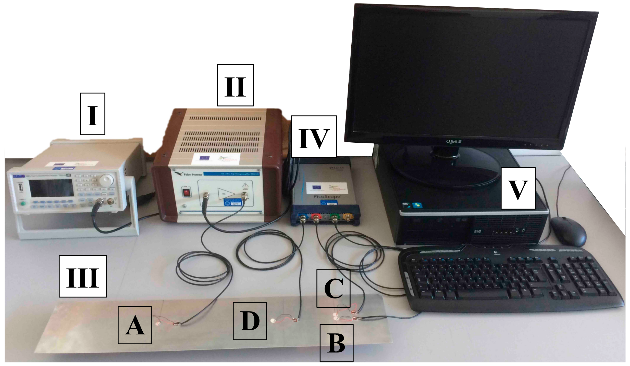
2.1.Experimental Set-Up

The experimental set-up is shown in the following Figure 1: I signal generator TG5012A (Aim & Thurlby Thandar Instrument); II power-amplifier Falco System WMA-300 (that multiplies by 50 the input voltage); III aluminium plate (with thickness equal to 1.2 mm and the following mechanical properties: E = 71 GPa; ρ = 2770 kg/m3; υ = 0.33); IV oscilloscope Serie 3000 PicoScope; V PC (using software PicoScope 6 and MATLAB codes).
The sensors (10 mm of diameter and 0.2 mm of thickness) used in this work, A, B, C, and D (see Figure 1 and Figure 2) were made of PIC255 (piezoelectric ceramic material) that corresponds to 600 series of EN50324 European Standard.
These PZTs have large charge coefficient, moderate permittivity and high coupling factor (the piezoelectric material is a soft ceramic with high domain mobility that allows a relatively easy polarization). The electrodes are wrapped-around on the same side in order to establish electrical contacting at a favourable position: in the following Table 1 the sensor properties are reported.
The “sensors status” is the main focus of this work: the sensor adhesion, with typical two-component epoxy glue, can fail for the quality of the metal and PZT surfaces preparation, for poor adhesive properties or a wrong bonding process: in most of the cases, the failure starts at the edge of the adhesive zone [24] (see Figure 2). For this reason, experimental specimens were manufactured with artificial damages by insertion of a thin Teflon patch between the sensor and the plate during the glue curing. In terms of adhesion area:
  • A and C Are fully bonded;
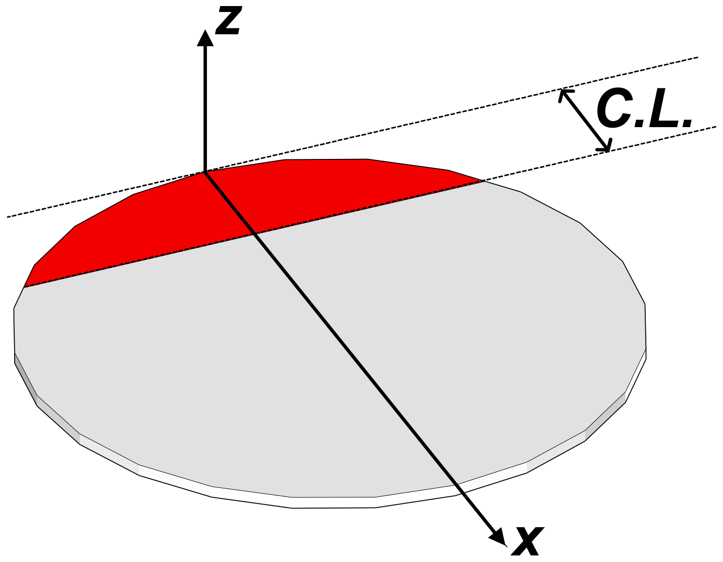
  • B is partially bonded, with an adhesive area equal to a circular segment with the “cut off” chord at 75% of the sensor diameter, along x-axis in Figure 3 (Teflon patch in red);
  • D is bonded for the half of the contact area.

2.2. SHM Techniques

2.2.1. ToF Evaluation Method

A 200 kHz-5 peaks toneburst was created by a MATLAB script and imported in the signal generator in order (i) to excite the fundamental Lamb modes (S0 and A0) on the aluminium plate by using sensor A, (ii) to ensure that the edge reflection waves do not overlap the S0 wave packet and (iii) to limit the phenomenon of velocity dispersion (see Figure 4, obtained by resolving Rayleigh—Lamb equation). In this case fd was equal to 0.24 MHzmm.
The amplitude signal was set to 150 Vpp. Single Trigger mode control allowed the oscilloscope to monitor the incoming signal on the other sensors (B and C), waiting for the voltage to rise above a set threshold. The received signals were post-processed in MATLAB. Short Time Fourier Transform (STFT) was used to evaluate the ToF [25] of S0 200 kHz packet wave to reach the impaired (B) and undamaged (C) sensors: signal differences between B and C outputs indicated the presence of a damaged sensor, i.e., signal delay suggested there was a bad working sensor.

2.2.2. Nonlinear Method by Using Subharmonics

In order to evaluate the acquisition system nonlinearities, PZTs A, B and D in Figure 2 were excited one at time (one sensor in exciting mode and the other two in receiving mode). When the sensor is partially debonded from the surface on to which it is applied, the debonded part, the red one in Figure 3, is free to move and can be considered as a cantilevered plate in motion under the action of external forces. Firstly, it was necessary to set a threshold below which the sensor could be considered “fully bonded”: a damage with Characteristic Length (C.L. in Figure 3) lower than 1 mm was set as not meaningful. In this manner, the first natural frequency associated with the debonded part of the sensor provided the lower frequency limit for the excitation signal as explained after in the paper.
In the case of a variable cross-section plate (as the red one in Figure 3), the bending natural frequency of the sensor debonded part is expressed by means of Rayleigh’s quotient [26] as:
f 2 = E ( 1 ν 2 ) 0 C . L . I y ( x ) [ d 2 g ( x ) d x 2 ] 2 d x 4 π 2 ρ 0 C . L . A ( x ) [ g ( x ) ] 2 d x
where E (65 GPa), ν (0.3) and ρ (7800 kg/m3) are elastic modulus, Poisson’s ratio and density of the sensor material, Iy(x) and A(x) are the variable cross-sectional moment of inertia and area that are measured at the generic abscissa x (see Figure 3), and are expressed as:
I y ( x ) = w ( x ) t 3 12   and   A ( x ) = w ( x ) t  
with w(x) being the variable width and t the constant thickness. g(x) is the distribution function of plate deflection. Equation (1) is quite versatile as it enables calculating the out-of-plane bending resonant frequency of cantilever plate whose cross-section vary continuously (w(x) defined by a single analytical profile). It can be shown (see [27] for more details) that the distribution function can generically be expressed in terms of compliances.
g ( x ) = C l ( x ) + κ E G C a ( x ) x C c ( x ) C l
where:
  • G is the shear modulus of the sensor material; κ is a coefficient to model the short-plate character of this structure and, for a rectangular cross-section, is equal to 5/6;
  • Cl is the linear compliance, and is calculated as the ratio between the free-end, out-of-plane deflection and the corresponding force applied at the same point about the same direction; Cl(x) is another linear compliance that is calculated as the ratio of the out-of-plane deflection at a generic point of abscissa x to the force that is applied at the cantilever free end;
  • Ca(x), the axial compliance, represents the ratio between the axial displacement at a point of abscissa x and the axial force that would be applied at the cantilever free end;
  • Cc(x), the cross compliance, is the ratio of the slope of the deformed cantilever being measured at the point of abscissa x to the free-end, out-of-plane force.
C l = 0 C . L . x 2 E I y ( x ) d x ;   C l ( x ) = x C . L . x 2 E I y ( x ) d x ; C a ( x ) = x C . L . 1 E A ( x ) d x ;   C c ( x ) = x C . L . x E I y ( x ) d x
Using Rayleigh’s quotient, the first natural frequency of the sensor debonded part with C.L. equal to 1 mm was 138 kHz. Debondings between the sensor and the plate characterized by C.L. bigger than 1 mm will have a first natural frequency smaller than 138 kHz (as suggested by the previous Equations). Keeping this in mind, the authors, for choosing the optimal excitation frequency, performed a frequency sweep between 180 and 220 kHz to collect the signals with the highest response amplitudes. Following these preliminary tests, the excitation signal to feed the actuating sensor was chosen harmonic at 200 kHz and 150 Vpp: if the structure would be linear, the response would be linear indeed. If some sensors are debonded, the clapping between them and the plate will lead to the appearance of superharmonics in the response. The signals detected at the receivers were then post-processed in MATLAB by using the Fast Fourier Transform (FFT) in order to catch the “fully bonded” sensor (by monitoring first superharmonic amplitude) as discussed and explained after. Successively, experimental campaigns (using harmonic signals) were carried out in order to find which exciting frequency fe (using the “fully bonded” sensor) causes one single dominant subharmonic fD in the structural response. Finally, when fe = fD, each nonlinear component in the spectrum corresponds with a specific sensor damage (using Equation (1)).

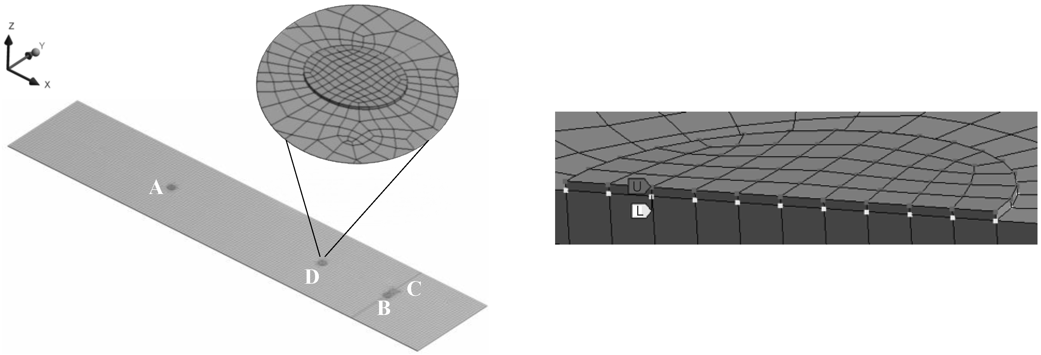
3. Numerical Simulations

The Finite Element Model (FEM) of the tested sample was created in Ansys Workbench where coupled field elements were used to study the PZTs acquisition system. Numerical models were implemented to simulate the piezoelectric and anisotropic behaviour of PZT sensors bonded on the structure. Command snippets were used to simulate the action of the experimental instruments.
The geometry was obtained by Design Modeler presented in Ansys Workbench. The aluminium plate was created by Extrude [28] feature and split by Face Split [28] in order to define PZT/structure interfaces and so the studied debonding. Cylindrical coordinate systems were defined on each sensor regarding to which the material properties were specified.
The aluminium plate was discretised by shell elements SHELL181 [28] suitable for analyses of thin to moderately-thick structures (see Figure 5—left). PZT disks were meshed by SOLID226 elements supporting piezoelectric physics combination (KEYOPTION (1) = 1001 for coupled-field piezoelectric analysis [28]). This element includes twenty nodes with Degrees of Freedom (DOFs) set by the field keys combination: piezoelectric DOFs are given by structural (field key = 1) and electrostatic (field key = 1000) field key.
The piezoelectric strain matrix [d in Table 1] was defined in Engineering Data and then converted to piezoelectric stress matrix before use and the anisotropic behaviour was taken into account defining the elasticity compliance matrix. All parts were meshed by Multizone method with hexagonal mapped mesh. A body sizing of 2 mm was used to discretise the aluminium plate and a sizing of 1 mm for the edges of the PZT/structure interfaces for a total of 10,885 nodes and 10,092 elements.
Ansys allows using several elements to model cases of changing mechanical contact between parts of an assembly or between different faces of a single part. The CONTA174 elements were used to mesh the contact between PZT sensors and structure.
Bonded contacts with Multi-Point-Constraint (MPC) [28] formulation were defined for undamaged sensors (A and C) and for the intact part of the adhesive interface at sensors B and D. MPC formulation is a direct and not penalty-based method that adds constraint equations to prevent relative displacements between contacting surfaces. Frictionless contact was used to model the debondings of PZT sensors. It has a unilateral behaviour for which normal pressure equals zero if separation occurs and leads to a nonlinear solution because the area of contact may change as the load is applied.
Named selections were used to select the nodes belonging to the upper and lower PZT surfaces. These were electrically constrained each other in order to define top and bottom electrodes. The PZT lower nodes (L in Figure 5—right) were grounded while the upper ones (U) were used to impose voltage or to detect signals.
Coupled-field models were implemented for solving problems where the coupled interaction of various physical phenomena, such as piezoelectricity, is important [29]. A direct formulation was used with elements having all the necessary DOF (displacements and charge) from which the appropriate element matrices and load vectors are calculated. The element matrix equations were derived by a strong coupling method [28]:
[ [ K 11 ] [ K 12 ] [ K 21 ] [ K 22 ] ] { { u } { V } } = { { F } { L } }
where {u} and {V} are the displacements and voltage respectively, {F} and {L} are the load vectors. The coupled effect is given by the presence of the off-diagonal submatrices [K12] and [K21] and calculated in one iteration.
Modal analyses were carried out in order to estimate the defect/damage first resonance frequency where only PZT sensors were modelled. The bonding with the aluminium plate was replaced by a definition of a fixed support on the interface. A resonance frequency of 130 kHz was calculated for the smallest C.L. (1 mm) classifiable as defect/damage in this work. The use of signals at higher frequencies allowed avoiding the excitation of a Local Defect Resonance (LDR) due to PZT debonding with C.L. bigger than 1 mm.
The experimental toneburst was imported in a Transient Structural analysis through *TREAD function and applied on the upper electrode of A sensor in order to simulate the fundamental Lamb modes (S0 and A0). In analysis settings, two steps were specified: the time length of the first equals the length of toneburst (5 Te where Te is the period of the used exciting packets) and those of the second one was fixed to 150 μs. The time step was fixed to Te/20 and the large displacement options was disabled. The received signals were obtained by detecting the voltage on the other sensors (B and C) and post-processed in MATLAB.
For the nonlinear method, Transient Structural analyses were carried out in order to evaluate the acquisition system nonlinearities by exciting PZTs one at time. Sensors were loaded by the same experimental harmonic signal, specified as a function in Workbench. The signals detected on the receivers were then post-processed in MATLAB by using the Fast Fourier Transform (FFT) in order to obtain the frequency spectra.

4. Results and Discussion

First of all, the sample was excited with the 200 kHz–5 peaks toneburst (sensor A in exciting mode), in order to compare the ToF between sensors B and C. The measurements were repeated five times to evaluate their consistency and robustness of the approach. If both the sensors would be intact, the ToF to B and C would be equal and this was tested before damaging the sensor B for calibrating the sample. The toneburst was imposed at the exciter and repeated with a frequency of 10 Hz (excitation generated every 0.1 s). The signal generator and the oscilloscope do not exchange information between them and this repeating technique is needed to catch at least one signal by the Picoscope. Signals with normalised amplitude and relative STFTs at 200 kHz are plotted in Figure 6 (Experimental and FEM cases). The differences between experimental and numerical time axes is due to the use of trigger in experiments that allows to register the sensor response when voltage on it exceeds a threshold level defined by the Picoscope. The S0 wave packet in Figure 6.a was picked up after about 1 ms from generator turning on. The sensor debonding affected the ToF needed for wave packet reaching B and C positions. As experimentally showed, there was an average time-shift of 1.6 microseconds with an uncertainty of ±0.2 microseconds: the signal arrived to B with a delay respect to the sensor C and this was expected since the B sensor was partially debonded. The numerical models confirmed the experimental results with a time-shift of 1.8 microseconds. The ToF variation can be actually used as an indicator of sensor debonding with some limitations:
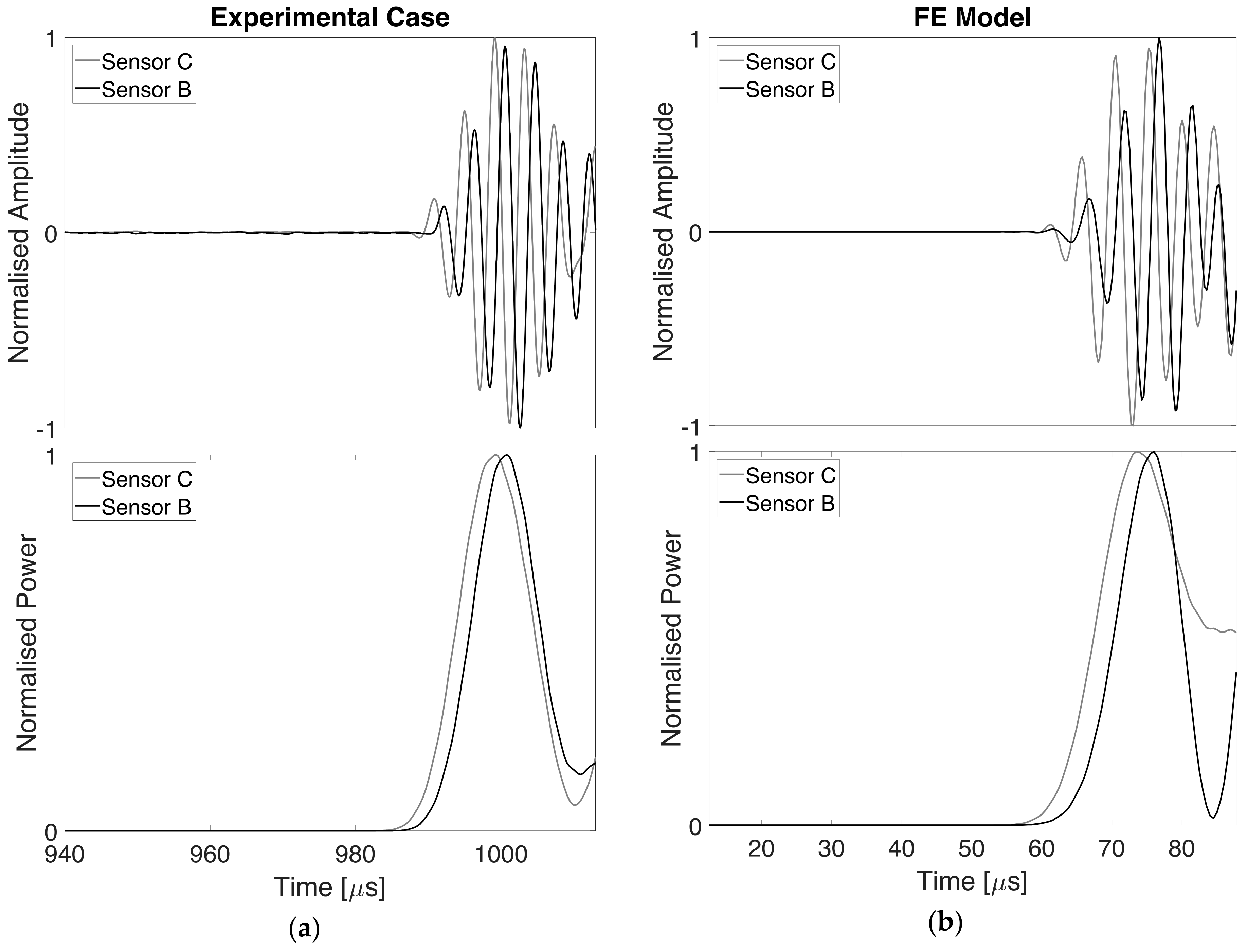
  • the ToF associated with the intact (fully bonded) sensor should be known a priori: in this way the time-shift (otherwise wrongly interpreted) allows to identify the damaged sensor;
  • the debonded region must be oriented to the exciting sensor like in the present case of investigation: the ToF actually indicates the presence of debonding when it occurs between approaching edge and propagation wavefront as reported also in [22]. If this condition is not satisfied, the ToF can be useless in the identification of impaired sensors;
  • a comparison with an undamaged sensor (in this case the sensor C) should be made to evaluate the time-shift, which makes this approach requiring a baseline.
To overcome the ToF technique limits, the harmonic analyses were carried out by exciting sensors A, B, and D, evaluating the nonlinearities in the acquired signals, due to the clapping between the damaged sensor and the aluminium plate. The first superharmonic amplitude in the receiver spectral response was used as nonlinear parameter. Also in this case the measurements were repeated five times and averaged for minimizing the noise effect and reducing the uncertainty.
As reported in Table 2, when A was used as actuator (i.e., exciter) and B and D were used as receivers, higher first superharmonics appeared in the receiver’s spectral response than when B and D were used as actuators. Both experimental and numerical results revealed a first superharmonic amplitude difference at least of 8 dBu corresponding to a 150% voltage difference. The relevant nonlinearities produced by sensor A in exciting mode indicated the presence of defect/damage that in this work can be associated only with the other sensors B and D since an undamaged aluminium plate was used as inspected structure and the electronic equipment feeding the actuating sensor did not produce in itself nonlinearities.
The excitation from B and D produced, both in experiments and numerical analyses, lower superharmonics in the receiver’s spectral response because of the damaged interface between them and the plate that does not allow a good energy transfer between the actuator and the structure. For these reasons, A, B, and D were identified respectively as fully bonded (undamaged) sensor and impaired sensors.
This suggests a procedure for the identification of impaired sensors in a typical SHM network of sensors.
The sensor A was then used to excite the structure and to characterise the debonding at sensors B and D interfaces. Differences between experimental and numerical signal amplitudes were due to the need of limiting the computational time using particular mesh sizing and contact parameters (not affecting indeed the correlation with the experimental results). As done in [30,31,32], the specimen was excited by harmonic voltage imposed at sensor A and the dynamic response was picked up at receivers B and D. The signal frequency was varied from 2.1 kHz to 138 kHz corresponding to the resonance frequency of sensors with C.L. respectively of 7.5 and 1 mm calculated analytically by Equation (1). The presence of subharmonic components (fD = fe/2 and multiplies of fD) in the frequency spectra would indicate LDR occurrence.
A first subharmonic appeared experimentally at an excitation frequency of 10.91 kHz: the spectrum of the signal acquired at the sensor B (Figure 7a) showed subharmonic components at multiples of 5.48 kHz; the spectrum in D (Figure 8a) exhibited the same behaviour with subharmonics at multiples of 5.43 kHz. The spectra obtained at an excitation frequency of 10.26 kHz by the FE models showed subharmonics at 5.13 kHz (Figure 7b and Figure 8b) that is in a good agreement with the experimental results. A second subharmonic appeared during experiments at fe equal to 39.98 kHz. In Figure 7c a component of 20.05 kHz was clearly identified in the spectrum of signal in B, while subharmonics occurred at multiplies of 19.94 kHz in the spectrum of signal in D (Figure 8c). Numerical simulations with fe equal to 40.94 kHz showed for the same cases a subharmonic frequency value of 20.51 and 20.52 kHz (Figure 7d and Figure 8d). The experimental results are in good agreement with the numerical ones (error of 6% in the worst case).
In order to understand the relation between LDRs and sensor B and D damages, harmonic analyses were carried out by exciting A at previously evaluated subharmonic frequencies and by monitoring the voltage at sensors B and D.
The amplitude responses to harmonic excitation are reported in Table 3:
  • the excitation at first subharmonic frequency (fe at 5.45 kHz in experiments and fe at 5.13 kHz in numerical simulations) led to voltage peak at sensor D higher than the received one at sensor B. The excitation at first subharmonic frequency (fe at 19.99 kHz in experiments and fe at 20.51 kHz in numerical simulations) led to voltage peak at sensor B higher than the received one at sensor D;
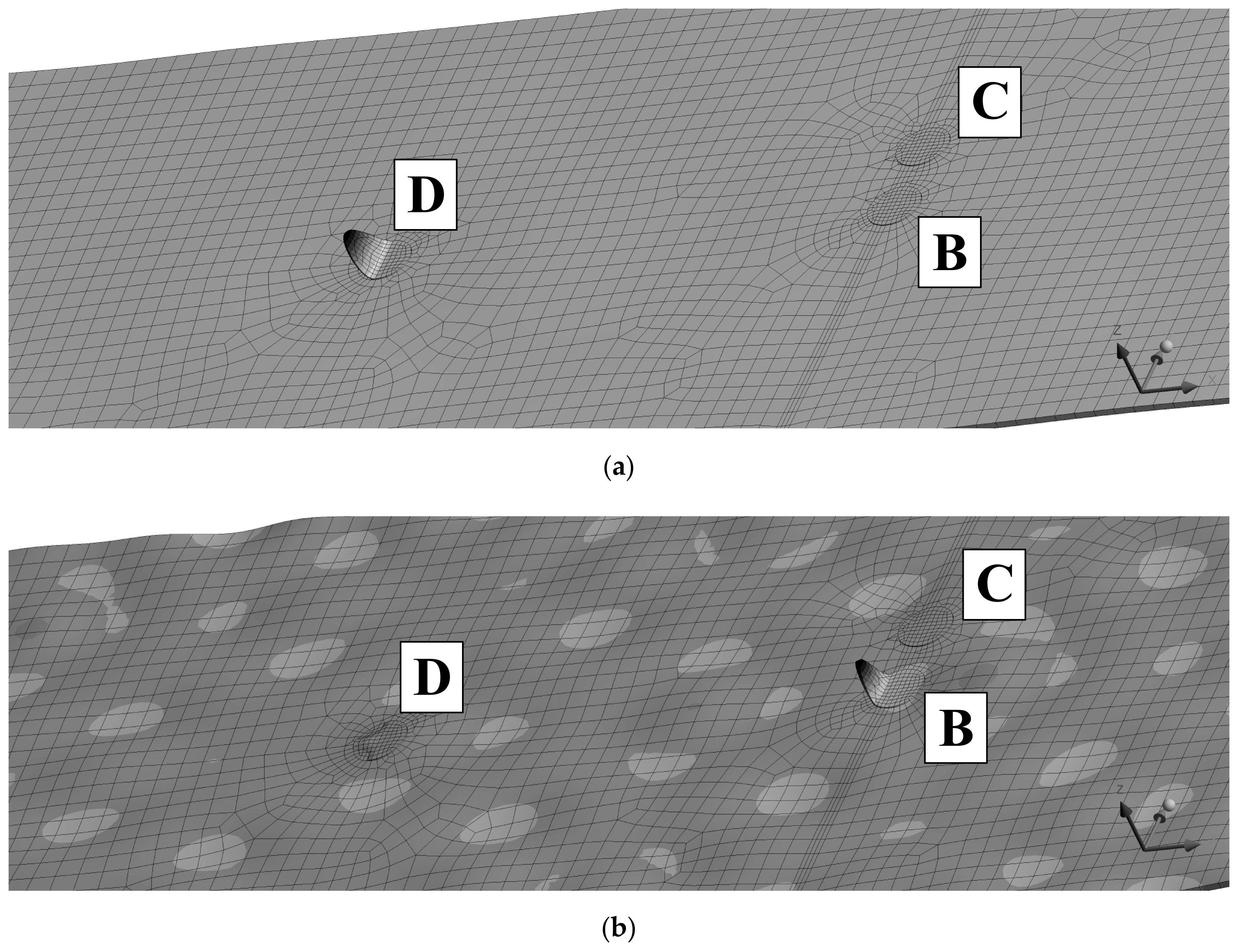
  • for every exciting frequency (experimental cases or FE models), the higher voltage peak was produced by the impaired sensor which was characterised by having the damage resonance frequency equal to fe (LDR). This happens because a structure excited at its natural frequency, behaves with abnormal vibrations (as highlighted in Figure 9): in the specific case of the present investigation, the excitation from the sensor A resulted in higher voltage peak of the impaired sensor since its frequency was equal to the first natural frequency of the sensor debonded part that was free to vibrate as a cantilevered plate.
Essentially the 5.45 kHz frequency observed experimentally was related to the damage on sensor D, the frequency 19.99 kHz was related to the damage on sensor B.
The final step of the damage identification was to evaluate C.L. at sensor B and D, using Equation (1), plotted in Figure 10 representing the natural frequency of a cantilevered plate for different values of C.L. In the first instance, the good correlation between analytical and numerical results is highlighted by the error bars (10%) in the graph. In the second instance, it is easy to conclude that the sensor (i.e., B or D) suffers damage with a specific C.L. provided by the chart in Figure 10 entering with the proper value of natural frequency experimentally found. Using this approach, the adhesive area of sensor B was estimated equal to a circular segment with the “cut off” chord at 74% of the sensor diameter (actual position of Teflon patch at 75%); while the adhesive area of sensor D was estimated equal to a circular segment with the “cut off” chord at 48.5% of the sensor diameter (actual position of Teflon patch at 50%).

5. Conclusions

Electronics can affect the efficiency of SHM systems if the electronic devices on which they are based do not work properly. In the present paper, techniques for the identification of impaired PZT sensors are experimentally tested and numerically simulated.
A novel method based on nonlinearities associated with impaired sensors is provided. The dynamic responses picked up at the damaged sensors showed the presence of higher harmonics and, in some particular case, of subharmonics [30]. This behaviour was due to nonlinear effects caused by the clapping contact between PZT and the structure. The nonlinearity of the acquisition system was evaluated by comparing the amplitude of the first superharmonic f1st = 2fe (with fe the excitation frequency) using a sensor as actuator and the others as receivers, testing different configurations. In this way, it was possible to evaluate the state of each PZT and then to distinguish the fully bonded sensors from those impaired. The identified undamaged sensor was then used to excite the others with harmonic signal sweeping up to high frequencies to find subharmonics induced by LDR ([31,32]). The presence of subharmonic at fD = fe/2 in the acquired signals allowed to detect and to characterise possible debondings of the sensors mounted on the structure. A harmonic excitation at fD frequency was then imposed to undamaged PZT and the responses of the other sensors were acquired: LDR was associated with the PZT signal with the highest fundamental amplitude in the entire spectrum. The method was validated by the good agreement between the experimental and numerical results. This technique, unlike ToF evaluation, does not depend on the damage positions. The debonded part of PZTs will be induced to vibration and thus to LDR regardless of its location and orientation respect to the exciting PZT.
The proposed method could provide a baseline-free detection tool for the identification of debonded sensors used in typical SHM networks consisting of numerous sensors mounted on large aircraft structures.

Author Contributions

Conceptualization, G.S.; methodology, G.S., S.C., and F.N.; software, S.C.; validation, F.N.; formal analysis, G.S., S.C., and F.N.; investigation, G.S., F.N., and S.C.; resources, G.S.; data curation, S.C. and F.N.; writing—original draft preparation, S.C. and F.N.; writing—review and editing, G.S.; visualization, G.S., S.C., and F.N.; supervision, G.S.; project administration, G.S.

Conflicts of Interest

The authors declare no conflict of interest.

References

  1. Abe, M. Structural monitoring of civil structures using vibration measurement Current practice and future. In Artificial Intelligence in Structural Engineering; Springer: Berlin/Heidelberg, Germany, 1998; pp. 1–18. ISBN 978-3-540-68593-7. [Google Scholar]
  2. Ostachowicz, W.; Kudela, P.; Krawczuk, M.; Zak, A. Guided Waves in Structures for SHM: The Time-Domain Spectral Element Method; John Wiley & Sons: New York, NY, USA, 2011; pp. 233–294. ISBN 978-0-470-97983-9. [Google Scholar]
  3. De Marchi, L.; Marzani, A.; Miniaci, M. A dispersion compensation procedure to extend pulse-echo defects location to irregular waveguides. NDT E Int. 2013, 54, 115–122. [Google Scholar] [CrossRef]
  4. Miniaci, M.; Gliozzi, A.S.; Morvan, B.; Krushynska, A.; Bosia, F.; Scalerandi, M.; Pugno, N.M. Proof of concept for an ultrasensitive technique to detect and localize sources of elastic nonlinearity using phononic crystals. Phys. Rev. Lett. 2017, 118, 214301. [Google Scholar] [CrossRef] [PubMed]
  5. Ciampa, F.; Mankar, A.; Marini, A. Phononic Crystal Waveguide Transducers for Nonlinear Elastic Wave Sensing. Sci. Rep. 2017, 7, 14712. [Google Scholar] [CrossRef] [PubMed] [Green Version]
  6. Senesi, M.; Xu, B.; Ruzzene, M. Experimental characterization of periodic frequency-steerable arrays for structural health monitoring. Smart Mater. Struct. 2010, 19, 055026. [Google Scholar] [CrossRef]
  7. Gliozzi, A.S.; Miniaci, M.; Bosia, F.; Pugno, N.M.; Scalerandi, M. Metamaterials-based sensor to detect and locate nonlinear elastic sources. Appl. Phys. Lett. 2015, 107, 161902. [Google Scholar] [CrossRef] [Green Version]
  8. Song, G.; Gu, H.; Mo, Y.L.; Hsu, T.T.; Dhonde, H. Concrete structural health monitoring using embedded piezoceramic transducers. Smart Mater. Struct. 2007, 16, 959. [Google Scholar] [CrossRef]
  9. Giri, P.; Kharkovsky, S.; Zhu, X.; Clark, S.M.; Taheri, S.; Samali, B. Characterization of carbon fiber reinforced polymer strengthened concrete and gap detection with a piezoelectric-based sensory technique. Struct. Health Monit. 2018, 11. [Google Scholar] [CrossRef]
  10. Wu, F.; Chang, F.K. Debond detection using embedded piezoelectric elements in reinforced concrete structures-part I: Experiment. Struct. Health Monit. 2006, 5, 5–15. [Google Scholar] [CrossRef]
  11. Wang, Y.; Zhu, X.; Hao, H.; Ou, J. Guided wave propagation and spectral element method for debonding damage assessment in RC structures. J. Sound Vib. 2009, 324, 751–772. [Google Scholar] [CrossRef]
  12. Adams, R.D.; Adams, R.D.; Comyn, J.; Wake, W.C. Structural Adhesive Joints in Engineering; Springer Science & Business Media: Dordrecht, The Netherlands, 1997; p. 244. ISBN 978-0-412-70920-3. [Google Scholar]
  13. Viana, G.M.; Costa, M.; Banea, M.D.; da Silva, L.F. A review on the temperature and moisture degradation of adhesive joints. Proc. Inst. Mech. Eng. Part L J. Mater. Des. Appl. 2017, 231, 488–501. [Google Scholar] [CrossRef]
  14. Tinoco, H.A.; Serpa, A.L.; Peña, F.M. Debonding estimation of piezoelectric sensors by power consumption analysis in smart structures using the finite element method. In Proceedings of the V Congreso Internacional de Ingenierıa Mecįnica y III de Ingenierıa Mecatronica, Colombia, Bogota, 11–12 August 2011; pp. 1–12. [Google Scholar]
  15. Overly, T.G.; Park, G.; Farrar, C.R. Development of signal processing tools and hardware for piezoelectric sensor diagnostic processes. Sens. Syst. Netw. Phenom. Technol. Appl. NDE Health Monit. 2007, 6530, 653018. [Google Scholar] [CrossRef]
  16. Wandowski, T.; Moll, J.; Malinowski, P.; Opoka, S.; Ostachowicz, W. Assessment of piezoelectric sensor adhesive bonding. J. Phys. Conf. Ser. 2015, 628, 012114. [Google Scholar] [CrossRef] [Green Version]
  17. Lanzara, G.; Yoon, Y.; Kim, Y.; Chang, F.K. Influence of interface degradation on the performance of piezoelectric actuators. J. Intell. Mater. Syst. Struct. 2009, 20, 1699–1710. [Google Scholar] [CrossRef]
  18. Park, G.; Farrar, C.R.; Rutherford, A.C.; Robertson, A.N. Piezoelectric active sensor self-diagnostics using electrical admittance measurements. J. Vib. Acoust. 2006, 128, 469–476. [Google Scholar] [CrossRef]
  19. Lee, S.J.; Sohn, H.; Michaels, J.E.; Michaels, T.E. In situ detection of surface–mounted pzt transducer defects using linear reciprocity. In AIP Conference Proceedings; AIP: Kingston, Rhode Island, 2010; Volume 1211, pp. 1844–1851. [Google Scholar]
  20. Lee, S.J.; Michaels, J.E.; Sohn, H.; Michaels, T.E. Piezoelectric transducer diagnostics via linear reciprocity for guided wave structural health monitoring. AIAA J. 2011, 49, 621–629. [Google Scholar] [CrossRef]
  21. Achenbach, J.A.; Achenbach, J.D. Reciprocity in Elastodynamics; Cambridge University Press: Cambridge, UK, 2003; pp. 90–115. ISBN 9780511550485. [Google Scholar]
  22. Sathyanarayana, C.N.; Ashwin, U.; Raja, S. Effect of sensor debonding on lamb wave propagation in plate structure. ARPN J. Eng. Appl. Sci. 2014, 9, 1358–1366. [Google Scholar]
  23. Giurgiutiu, V. Structural Health Monitoring with Piezoelectric Wafer Active Sensors; Elsevier: Burlington, MA, USA, 2007; pp. 321–329. [Google Scholar]
  24. Scarselli, G.; Corcione, C.; Nicassio, F.; Maffezzoli, A. Adhesive joints with improved mechanical properties for aerospace applications. Int. J. Adhes. Adhes. 2017, 75, 174–180. [Google Scholar] [CrossRef]
  25. Duarte, R.M.; Villanueva, J.M.; Costa, M.M.; Freire, R.C.; Catunda, S.Y.; Costa, W.M. Ultrasonic time of flight estimation for wind speed measurement based on time-frequency domain using STFT. In Proceedings of the 19th IMEKO TC 4Symposium and 17th IWADC Workshop Advances in Instrumentation and Sensors Interoperability, Barcelona, Spain, 15 July 2013; pp. 18–19. [Google Scholar]
  26. Lobontiu, N.; Ilic, B.; Reissman, T.; Garcia, E.; Nam, Y.; Craighead, H.G. Modeling, Design and Experimental Characterization of Bending Resonant Circular Nano Cantilevers. Micro Nanosyst. 2009, 1, 22–29. [Google Scholar] [CrossRef]
  27. Lobontiu, N. Compliant Mechanisms: Design of Flexure Hinges; CRC Press: Boca Raton, FL, USA, 2002; pp. 214–215. ISBN 9780849313677. [Google Scholar]
  28. ANSYS Help. Available online: https://ansyshelp.ansys.com (accessed on 30 August 2018).
  29. Chien, W.T.; Yang, C.J.; Yen, Y.T. Coupled-field analysis of piezoelectric beam actuator using FEM. Sens. Actuators A Phys. 2005, 118, 171–176. [Google Scholar] [CrossRef]
  30. Ciampa, F.; Scarselli, G.; Meo, M. On the generation of nonlinear damage resonance intermodulation for elastic wave spectroscopy. J. Acoust. Soc. Am. 2017, 141, 2364–2374. [Google Scholar] [CrossRef] [PubMed] [Green Version]
  31. Scarselli, G.; Ciampa, F.; Nicassio, F.; Meo, M. Non-linear methods based on ultrasonic waves to analyse disbonds in single lap joints. Proc. Inst. Mech. Eng. Part C J. Mech. Eng. Sci. 2017, 231, 3066–3076. [Google Scholar] [CrossRef]
  32. Scarselli, G.; Ciampa, F.; Ginzburg, D.; Meo, M. Non-destructive testing techniques based on nonlinear methods for assessment of debonding in single lap joints. In Proceedings of the Structural Health Monitoring and Inspection of Advanced Materials, Aerospace, and Civil Infrastructure, San Diego, CA, USA, 1 April 2015; International Society for Optics and Photonics: San Diego, CA, USA, 2015; p. 943706. [Google Scholar]
Figure 1. Experimental set-up.
Electronics 07 00303 g001
Figure 2. Sample dimensions.
Electronics 07 00303 g002
Figure 3. Characteristic Length (C.L.) of damaged sensor.
Electronics 07 00303 g003
Figure 4. Rayleigh–Lamb curves: (top) wave speed and (bottom) group velocity dispersion curves.
Electronics 07 00303 g004
Figure 5. Meshing of plate and sensor (left) and Section on Plane XZ of Sensor Model (right).
Electronics 07 00303 g005
Figure 6. S0 packet and Short Time Fourier Transform (STFT) at 200 kHz for (a) experimental results and (b) Finite Element Model (FEM) data.
Electronics 07 00303 g006
Figure 7. Experimental (fe = 10.91 kHz in (a) and fe = 39.98 kHz in (c)) and FEM (fe = 10.26 kHz in (b) and fe = 40.94 kHz in (d)) spectra for subharmonic detection at sensor B.
Electronics 07 00303 g007
Figure 8. Experimental (fe = 10.91 kHz in (a) and fe = 39.98 kHz in (c)) and FEM (fe = 10.26 kHz in (b) and fe = 40.94 kHz in (d)) spectra for subharmonic detection at sensor D.
Electronics 07 00303 g008
Figure 9. FE simulation of harmonic excitation at 5.13 kHz (a) and 20.51 kHz (b).
Electronics 07 00303 g009
Figure 10. Analytical results (see Equation (1)) and FEM data.
Electronics 07 00303 g010
Table 1. Properties of PIC255.
Mechanical PropertiesDielectric Properties
Density
ρ [kg/m3]
7800Elastic Compliance
S33 [m2/N]
20.7 × 10⁻¹²Curie Temperature
[K]
623Relative Permittivity1650
Elastic Compliance
S11 [m2/N]
16.1 × 10⁻¹²Elastic Stiffness
E33 [N/m2]
10.0 × 10¹⁰Relative Permittivity1750Dielectric Loss Factor20 × 10−3
Electromechanical properties
Coupling factorPiezoelectric charge coefficientPiezoelectric Voltage Coefficient
kp0.62k330.69d31 [C/N]−180 × 10−12g31 [Vm/N]−11.3 × 10−3
kt0.47k150.66d33 [C/N]400 × 10−12g33 [Vm/N]25.0 × 10−3
k310.35d15 [C/N]550 × 10−12
Table 2. First superharmonic amplitude for nonlinear method.
Actuator (Exciter)ReceiverExperimental First Superharmonic Amplitude [dBu]Numerical First Superharmonic Amplitude [dBu]
AB−33.8−44.5
D−40.2−43.5
BA−54.0−55.7
D−53.2−56.1
DA−52.0−56.9
B−51.6−55.3
Table 3. Fundamental amplitude with fe equal to subharmonic frequencies.
Actuator (Exciter)ReceiverExperimentalNumerical
fe [kHz]Fundamental Amplitude [dBu]fe [kHz]Fundamental Amplitude [dBu]
AB5.45−20.25.13−18.7
D−15.1−13.3
B19.99−16.120.51−14.2
D−27.4−26.3

