Demodulation of Angular Position and Velocity from Resolver Signals via Chebyshev Filter-Based Type III Phase Locked Loop


Abstract
:1. Introduction
2. Resolver Principles and Problem Formulation
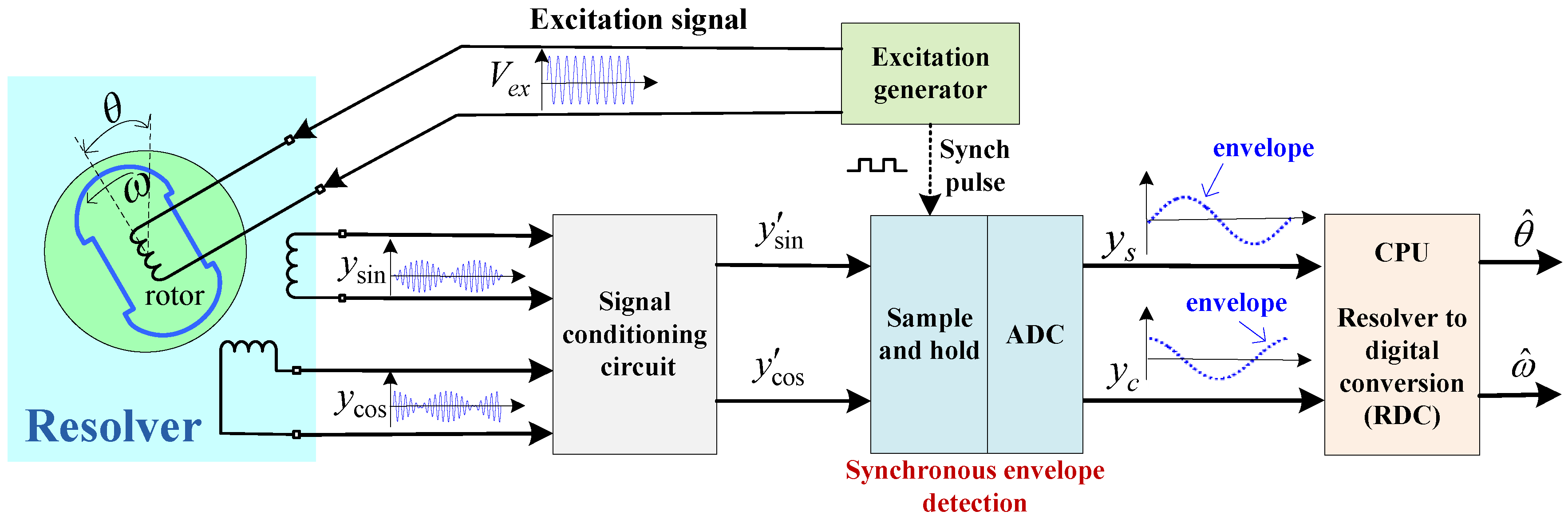
2.1. Principle of Resolver and Software-Based RDC
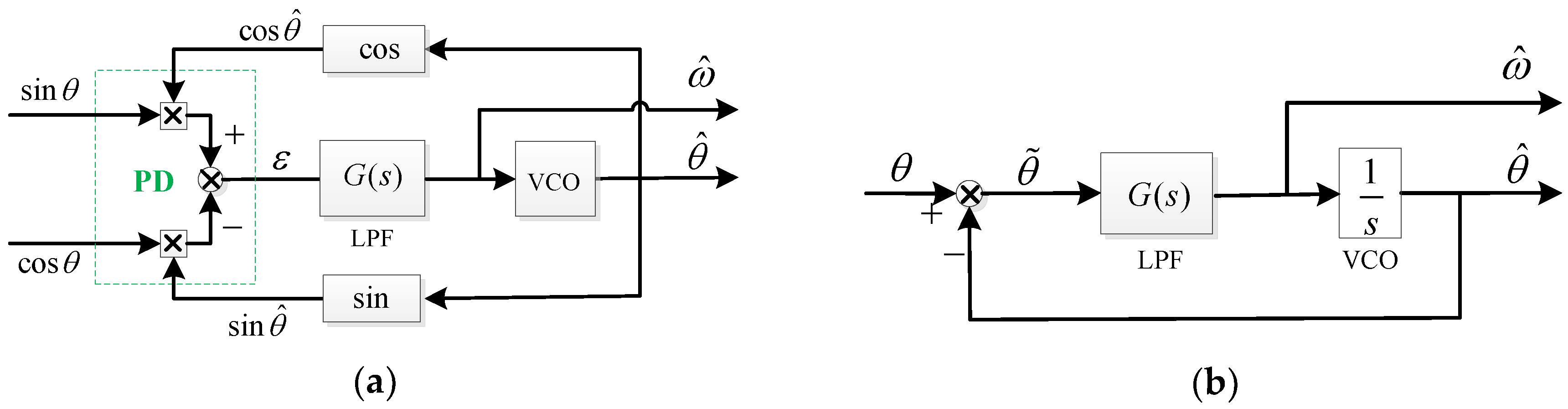
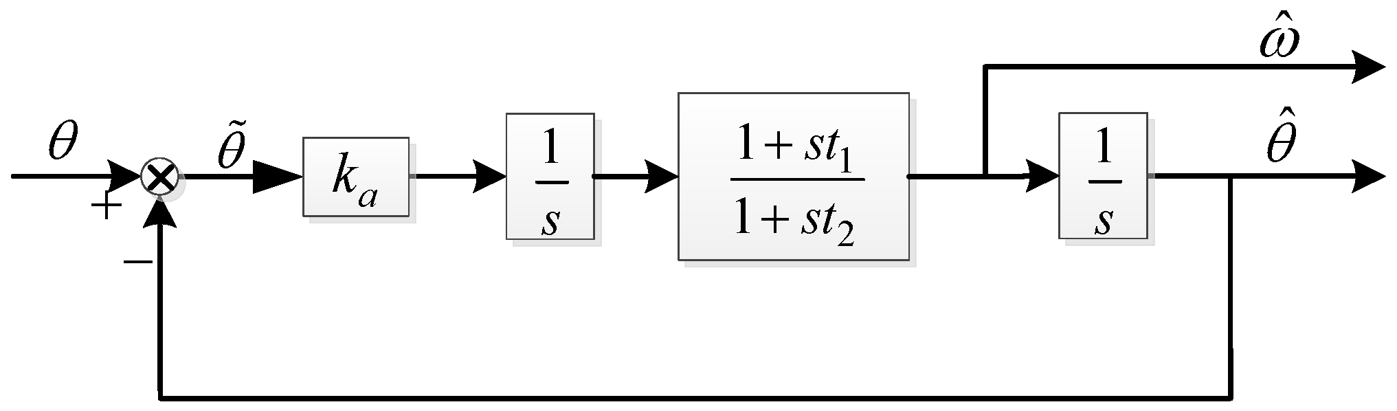
2.2. Review of Conventional PLL-Based Demodulation Method
3. Design of Chebyshev Filter-Based Type III PLL for Demodulation
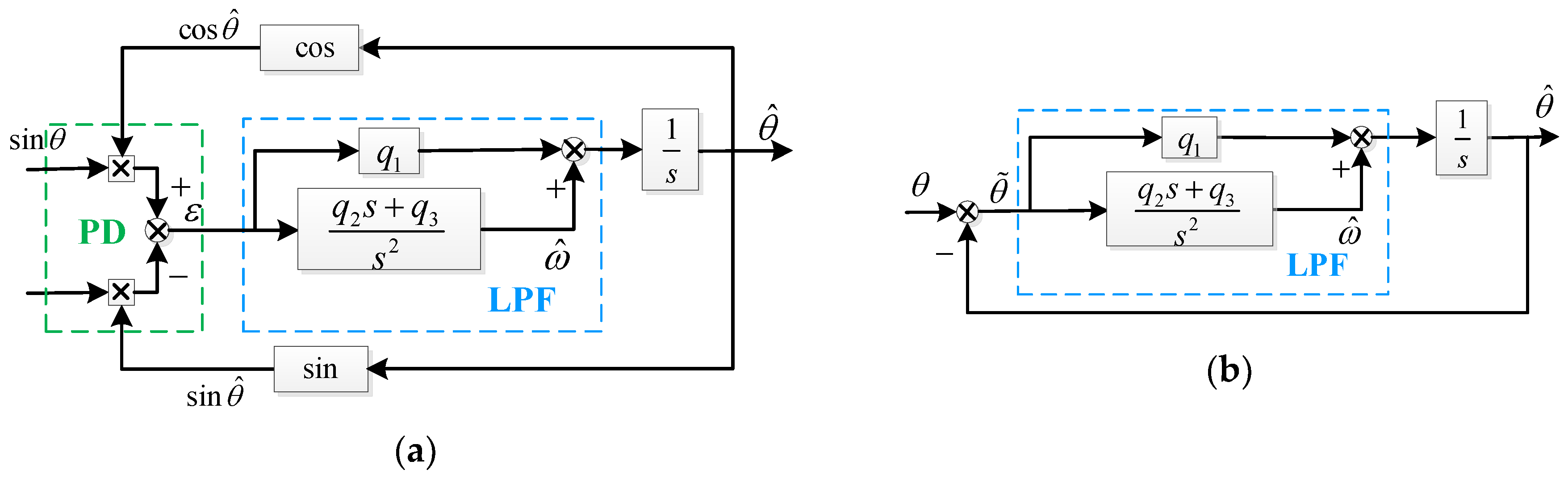
3.1. Design of Type III PLL
3.2. Parameter Design of Type III PLL via Chebyshev Filter
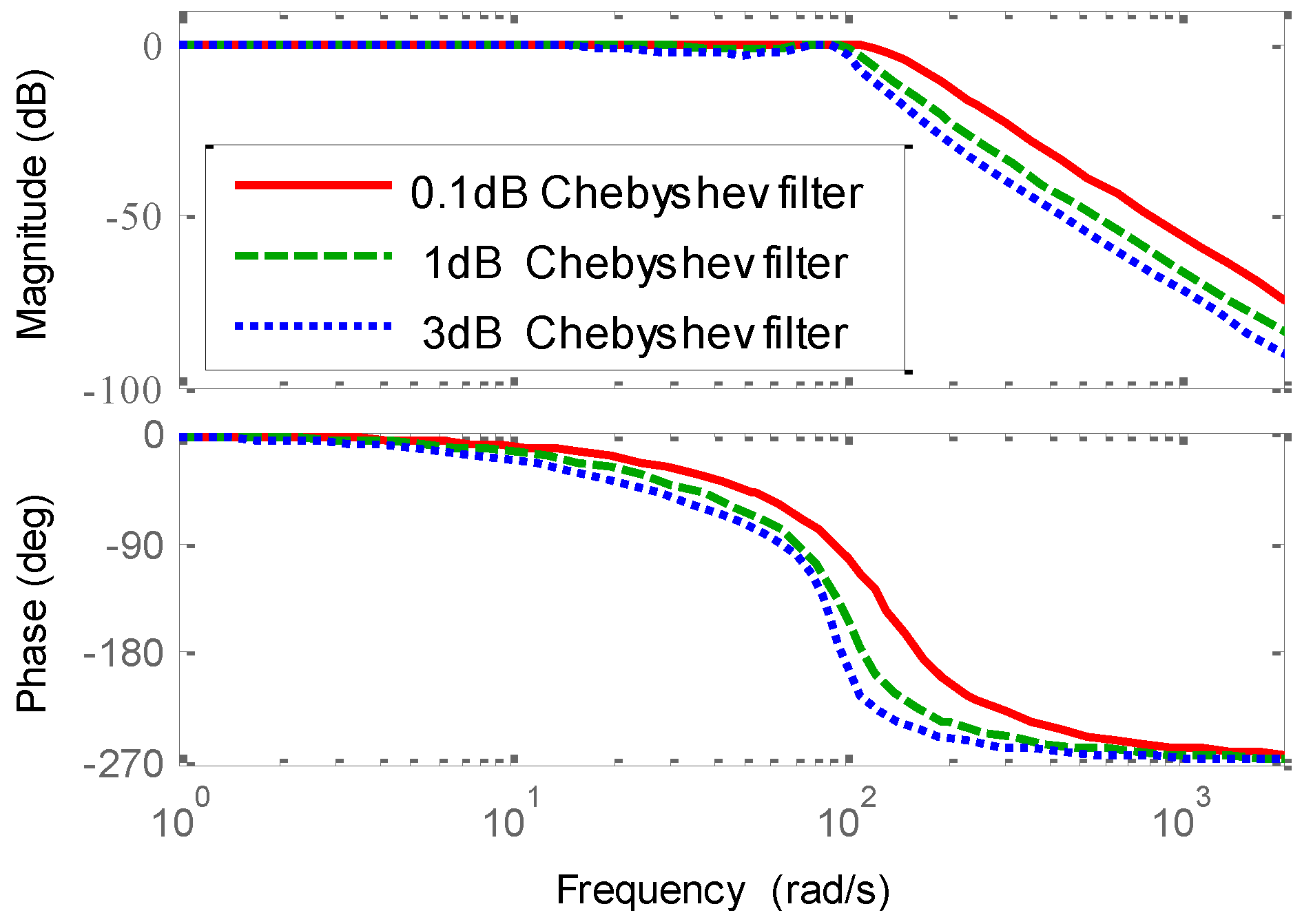
3.2.1. Introduction to Chebyshev Filter
3.2.2. Parameter Design of Type III PLL
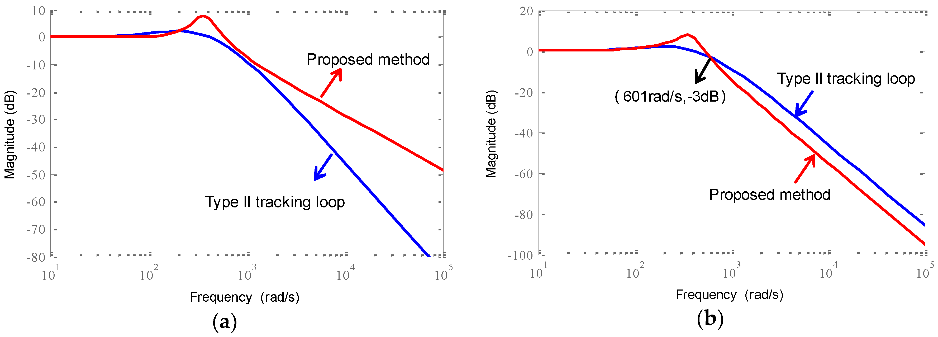
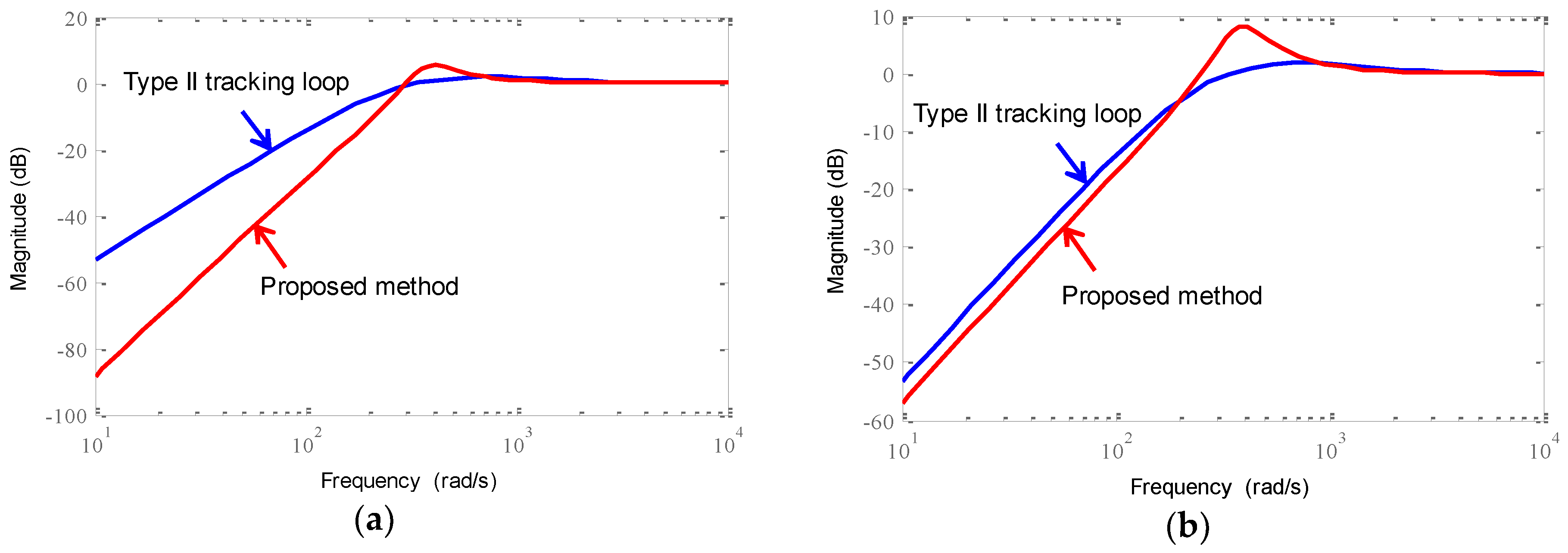
3.3. Performance Analysis of the Proposed Method
4. Simulation and Experimental Results
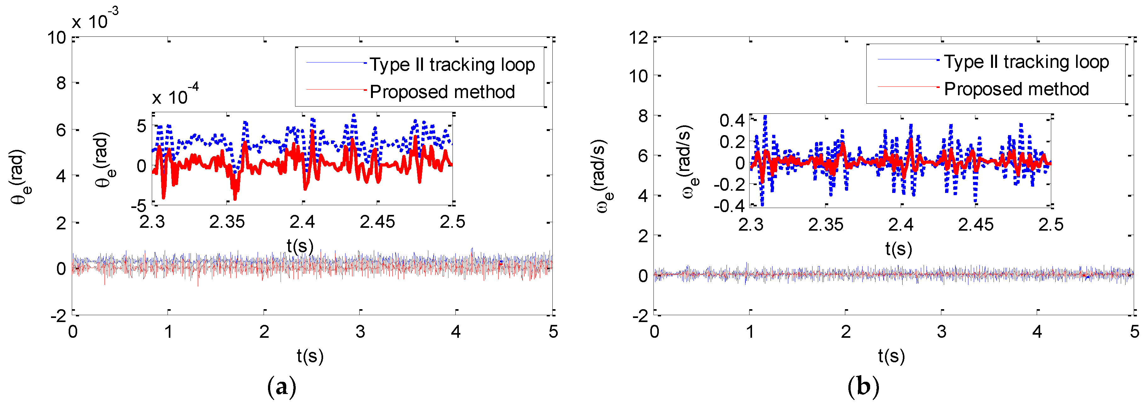
4.1. Simulation
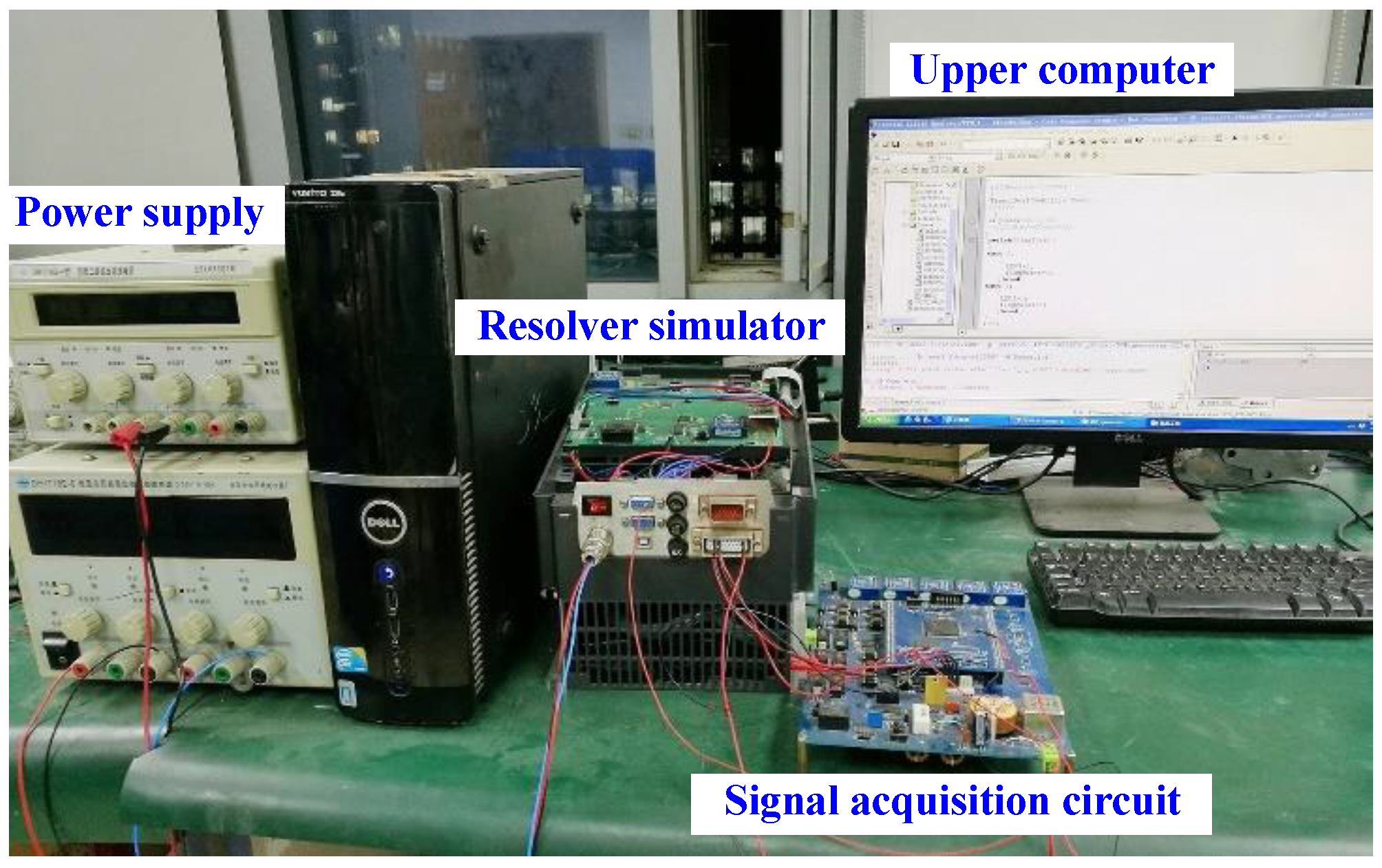
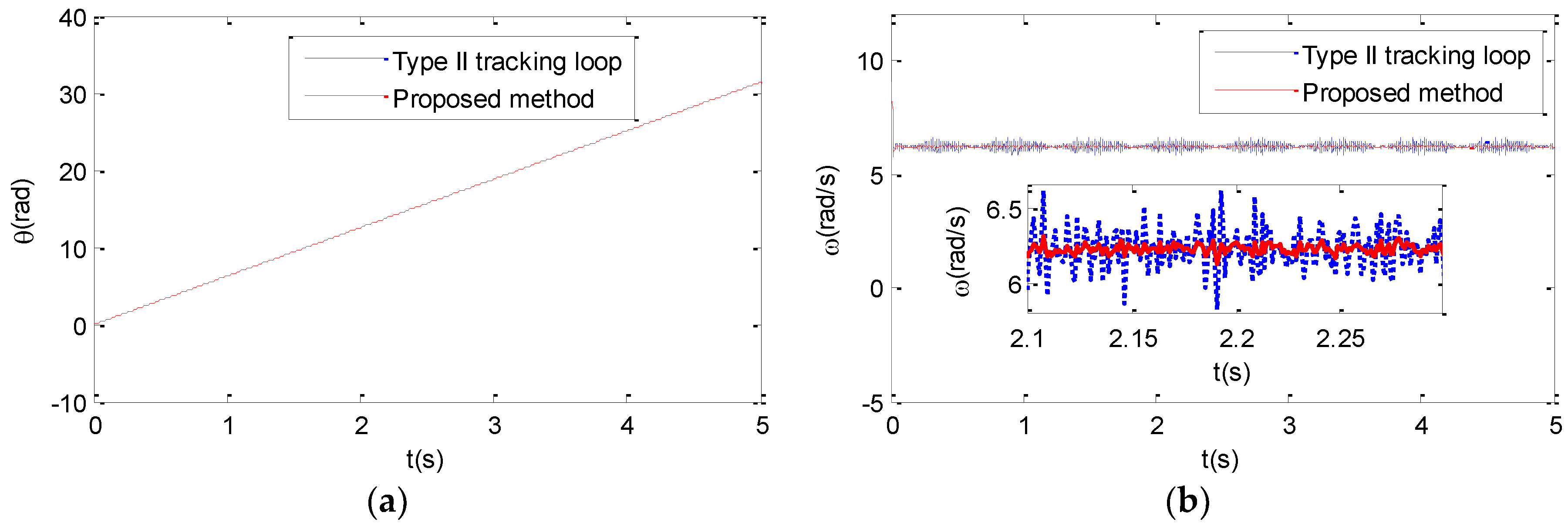
4.2. Experiment
5. Conclusions
Author Contributions
Funding
Conflicts of Interest
References
- Han, S.; Han, S. Resolver angle estimation using parameter and state estimation. Measurement 2016, 93, 460–464. [Google Scholar] [CrossRef]
- Benammar, M.; Ben-Brahim, L.; Alhamadi, M.A. A novel resolver-to-360° linearized converter. IEEE Sens. J. 2004, 4, 96–101. [Google Scholar] [CrossRef]
- Caruso, M.; Di Tommaso, A.O.; Genduso, F.; Miceli, R.; Galluzzo, G.R. A DSP-Based Resolver-To-Digital Converter for High-Performance Electrical Drive Applications. IEEE Trans. Ind. Electron. 2016, 63, 4042–4051. [Google Scholar] [CrossRef]
- Bergas-Jané, J.; Ferrater-Simón, C.; Gross, G.; Ramírez-Pisco, R.; Galceran-Arellano, S.; Rull-Duran, J. High-Accuracy All-Digital Resolver-to-Digital Conversion. IEEE Trans. Ind. Electron. 2012, 59, 326–333. [Google Scholar] [CrossRef]
- Ellis, G. Encoders and Resolvers. In Control System Design Guide, 4th ed.; Butterworth-Heinemann: Boston, MA, USA, 2012; Volume 14, pp. 285–311. [Google Scholar]
- Khaburi, D.A. Software-Based Resolver-to-Digital Converter for DSP-Based Drives Using an Improved Angle-Tracking Observer. IEEE Trans. Instrum. Meas. 2012, 61, 922–929. [Google Scholar] [CrossRef]
- Guo, C.; Wu, C.; Ni, F.; Liu, H. Software-based resolver-to-digital conversion and online fault compensation. In Proceedings of the 2016 IEEE International Conference on Mechatronics and Automation, Harbin, China, 7–10 August 2016; pp. 344–349. [Google Scholar]
- Sivappagari, C.M.R.; Konduru, N.R. Review of RDC soft computing techniques for accurate measurement of resolver rotor angle. Sens. Transducers 2013, 150, 1–11. [Google Scholar]
- Sarma, S.; Agrawal, V.K.; Udupa, S. Software-based resolver-to-digital conversion using a dsp. IEEE Trans. Ind. Electron. 2008, 55, 371–379. [Google Scholar] [CrossRef]
- Benammar, M.; Khattab, A.; Saleh, S.; Bensaali, F.; Touati, F. A Sinusoidal Encoder-to-Digital Converter Based on an Improved Tangent Method. IEEE Sens. J. 2017, 17, 5169–5179. [Google Scholar] [CrossRef]
- Pecly, L.; Schindeler, R.; Cleveland, D.; Hashtrudizaad, K. High-precision resolver-to-velocity converter. IEEE Trans. Instrum. Meas. 2017, 66, 2917–2928. [Google Scholar] [CrossRef]
- Karabeyli, F.A.; Alkar, A.Z. Enhancing the accuracy for the open-loop resolver to digital converters. J. Electr. Eng. Technol. 2018, 13, 192–200. [Google Scholar]
- Sun, J.D.; Cao, G.Z.; Huang, S.D.; Qiu, H. Software-based resolver-to-digital converter using the PLL tracking algorithm. In Proceedings of the International Conference on Ubiquitous Robots and Ambient Intelligence, Xi’an, China, 19–22 August 2016; pp. 719–723. [Google Scholar]
- Qamar, N.A.; Hatziadoniu, C.J.; Wang, H. Speed Error Mitigation for a DSP-Based Resolver-to-Digital Converter Using Autotuning Filters. IEEE Trans. Ind. Electron. 2015, 62, 1134–1139. [Google Scholar] [CrossRef] [Green Version]
- Benammar, M.; Gonzales, A.S.P. A Novel PLL Resolver Angle Position Indicator. IEEE Trans. Instrum. Meas. 2016, 65, 123–131. [Google Scholar] [CrossRef]
- Alemadi, N.; Benbrahim, L.; Benammar, M. A new tracking technique for mechanical angle measurement. Measurement 2014, 54, 58–64. [Google Scholar] [CrossRef]
- Harnefors, L.; Nee, H.P. A general algorithm for speed and position estimation of AC motors. IEEE Trans. Ind. Electron. 2000, 47, 77–83. [Google Scholar] [CrossRef]
- Zhang, J.; Wu, Z. Composite state observer for resolver-to-digital conversion. Meas. Sci. Technol. 2017, 28, 065103. [Google Scholar] [CrossRef]
- Raymundo, C.G.; João, O.P.P.; Suemitsu, W.I.; Soares, J.O. Improved demultiplexing algorithm for hardware simplification of sensored vector control through frequency-domain multiplexing. IEEE Trans. Ind. Electron. 2017, 64, 6538–6548. [Google Scholar]
- Tiapkin, M.G.; Balkovoi, A.P. High resolution processing of position sensor with amplitude modulated signals of servo drive. In Proceedings of the 2017 IEEE Conference of Russian Young Researchers in Electrical and Electronic Engineering (EIConRus), St. Petersburg, Russia, 1–3 February 2017; pp. 1042–1047. [Google Scholar]
- Alipour-Sarabi, R.; Nasiri-Gheidari, Z.; Tootoonchian, F.; Oraee, H. Performance Analysis of Concentrated Wound-Rotor Resolver for Its Applications in High Pole Number Permanent Magnet Motors. IEEE Sens. J. 2017, 17, 7877–7885. [Google Scholar] [CrossRef]
- Wu, Z.; Li, Y. High-Accuracy Automatic Calibration of Resolver Signals via Two-Step Gradient Estimators. IEEE Sens. J. 2018, 18, 2883–2891. [Google Scholar] [CrossRef]
- AD2S1210 Data Sheet: Variable Resolution, 10-Bit to 16-Bit R/D Converter with Reference Oscillator; Analog Devices, Inc.: Norwood, MA, USA, 2008; Available online: www.analog.com (accessed on 25 October 2018).
- Kawakami, M. Nomographs for Butterworth and Chebyshev Filters. IEEE Trans. Circuit Theory 1963, 10, 288–289. [Google Scholar] [CrossRef]
- Yahagi, T.; Wang, Y. Digital Filters and Signal Processing; The Science Publishing Company: Beijing, China, 2003; pp. 23–36. [Google Scholar]
- Liu, H.; Wu, Z. On estimation algorithm of angular velocity for servo motors with resolvers. In Proceedings of the Chinese Control and Decision Conference, Shenyang, China, 9–11 June 2018; pp. 4019–4024. [Google Scholar]


| 0.1 | 1.93881 | 2.62949 | 1.63805 |
| 0.5 | 1.25291 | 1.53490 | 0.71569 |
| 1 | 0.98834 | 1.23841 | 0.49131 |
| 2 | 0.73782 | 1.02219 | 0.32689 |
| 3 | 0.59724 | 0.92835 | 0.25059 |
| Cases | Estimation Error | Type II Tracking Loop | Proposed Method | ||
|---|---|---|---|---|---|
| AVG | STD | AVG | STD | ||
| Case 1 | Position estimation error (rad) | 1.951 × 10⁻⁷ | 9.302 × 10⁻⁵ | 1.877 × 10⁻⁷ | 1.073 × 10⁻⁴ |
| Velocity estimation error (rad/s) | −4.073 × 10⁻⁵ | 0.0927 | −2.112 × 10⁻⁵ | 0.0340 | |
| Case 2 | Position estimation error (rad) | 2.714 × 10⁻⁴ | 9.416 × 10⁻⁵ | 3.424 × 10⁻⁷ | 1.085 × 10⁻⁴ |
| Velocity estimation error (rad/s) | 5.738 × 10⁻⁵ | 0.0936 | 3.207 × 10⁻⁵ | 0.0348 | |
| PMSM | Resolver | ||
|---|---|---|---|
| Pole pairs | 2 | Pole pairs | 1 |
| Rated voltage | 110 V(AC) | Input voltage | 5 V ± 0.2 V (AC) |
| Rated speed | 3000 r/min | Input freguency | 10 kHz |
| Torque constant | 0.15 Nm/A | Ouput voltage | >2 V |
| Phase resistance | 8 Ω | Transformer raio | 0.5 ± 5% |
| Phase inductance | 10 mH | Electrical error | |
| Demodulation Methods | AVG | STD |
|---|---|---|
| Type II tracking loop | 6.23 | 0.105 |
| Proposed method | 6.23 | 0.0319 |
© 2018 by the authors. Licensee MDPI, Basel, Switzerland. This article is an open access article distributed under the terms and conditions of the Creative Commons Attribution (CC BY) license (http://creativecommons.org/licenses/by/4.0/).
Share and Cite
Liu, H.; Wu, Z. Demodulation of Angular Position and Velocity from Resolver Signals via Chebyshev Filter-Based Type III Phase Locked Loop. Electronics 2018, 7, 354. https://doi.org/10.3390/electronics7120354
Liu H, Wu Z. Demodulation of Angular Position and Velocity from Resolver Signals via Chebyshev Filter-Based Type III Phase Locked Loop. Electronics. 2018; 7(12):354. https://doi.org/10.3390/electronics7120354
Chicago/Turabian StyleLiu, Huan, and Zhong Wu. 2018. "Demodulation of Angular Position and Velocity from Resolver Signals via Chebyshev Filter-Based Type III Phase Locked Loop" Electronics 7, no. 12: 354. https://doi.org/10.3390/electronics7120354
APA StyleLiu, H., & Wu, Z. (2018). Demodulation of Angular Position and Velocity from Resolver Signals via Chebyshev Filter-Based Type III Phase Locked Loop. Electronics, 7(12), 354. https://doi.org/10.3390/electronics7120354