High-Order Sliding Mode-Based Fixed-Time Active Disturbance Rejection Control for Quadrotor Attitude System

Abstract

This article presents a fixed-time active disturbance rejection control approach for the attitude control problem of quadrotor unmanned aerial vehicle in the presence of dynamic wind, mass eccentricity and an actuator fault. The control scheme applies the feedback linearization technique and enhances the performance of the traditional active disturbance rejection control (ADRC) based on the fixed-time high-order sliding mode method. A switching-type uniformly convergent differentiator is used to improve the extended state observer for estimating and attenuating the lumped disturbance more accurately. A multivariable high-order sliding mode feedback law is derived to achieve fixed time convergence. The timely convergence of the designed extended state observer and the feedback law is proved theoretically. Mathematical simulations with detailed actuator models and real time experiments are performed to demonstrate the robustness and practicability of the proposed control scheme.

1. Introduction

Unmanned aerial vehicles (UAVs) are useful for tasks that are dangerous or unaccessible for human operation and popular in military and civilian applications such as investigation, inspection and surveillance with the advantage of moving in three-dimensional space flexibly. A quadrotor is a kind of vertical takeoff and landing (VTOL) aircraft lifted and controlled by four rotors [1]. Being simpler in structure, less sensitive to damage, easier to handle and more cost-effective, quadrotors have gained more attention in small unmanned aerial system (UAS) research than traditional helicopters. Therefore, plenty of remarkable research achievements related to quadrotors have been made in recent years [2,3].

In practical terms, the position control method is designed according to specific mission requirements and could be implemented onboard or remotely, while the attitude control is performed via an onboard processor to stabilize the attitude reliably [4]. Traditional efficient proportional–derivative (PD) control method has been used in the attitude control of quadrotor [5,6] and achieves good practical performance. Feedback linearization is a commonly used technique to control non-linear coupled systems and are adaptable to the controller design of quadrotor [7]. In [8], the attitude states are transformed into a new state space with a nonlinear transformation to obtain a linear system on which linear error-feedback control can be applied. The idea to design a controller on a transformed linear system instead of the original non-linear system is valuable, however the results in [8] show that the linear error-feedback controller is not robust in terms of uncertainties and measurement noises.

The small low-cost quadrotor is a non-redundant aircraft which suffers from external and internal disturbances such as dynamic wind and actuator faults. In order to design the attitude controller to be robust against unknown disturbances, the observer-based online disturbance estimation and attenuation strategies have been widely studied in recent years. A disturbance observer based on Q-filter is applied in [9,10] for robust hovering control. In [11], a neural network is used to learn the uncertain terms in UAV dynamics. Aboudonia integrated a disturbance observer with feedback linearization-based control in [12] for robustness, and combined a sliding mode controller with a disturbance observer in [13]. The control schemes are verified with the Dryden turbulence model and Von-Karman wind model, respectively. Disturbance observer-based trajectory tracking methods were studied in [14,15]. The sliding mode-based observer and high-order sliding mode-based observer are also extensively studied to enhance the robustness of feedback linearization-based controller [16], sliding mode controller [17] and back-stepping controller [18]. Shi designed extended state observers in [19,20] for the attitude control problem of quadrotors.

Active disturbance rejection control (ADRC) is proposed by Han in 2009 [21]. ADRC inherits from the classical proportional–integral–derivative (PID) controller and executes in an error-driven manner. By augmenting the system uncertainty into the state vector and constructing an extended state observer (ESO), the uncertainty is observed in real-time. Aiming at replacing PID in industrial applications, the ADRC scheme is developed experimentally in the first place. Recently, Guo [22] has proved the convergence of ADRC for non-linear systems mathematically. As a practical control scheme, ADRC has been applied to many engineering aspects, such as motor control, power plant control, ship control, etc [23] (pp. 6–9). ADRC has been adopted for attitude control of a quadrotor directly in [23,24,25,26].

In order to avoid the chattering effect in the sliding mode method, Levant [27,28] designed a general-form arbitrary-order exact robust differentiator based on high-order sliding mode (HOSM) algorithm. The proposed differentiator was proved to converge in finite time with bounded uncertainties. In [29], Levant’s robust differentiator was improved via an extra exponential function with an exponent greater than 1 in order to achieve fixed-time convergence regardless of the initial deviation. In [30], a kind of fixed-time observer is derived and the constraints of the corrective term is formulated. In fact, the observer in [29] is an instance of the formula of the fixed-time observer in [30]. Angulo designed a fixed-time observer operated in a switching manner in [31]. The observer is switched from a uniform differentiator to Levant’s finite-time differentiator. Compared with the methods used in [29,30], Angulo’s switching-type observer performs only one exponential function at each step. Therefore, it is more practical on micro-processors with limited computing power. The switching-type observer has been applied to hypersonic vehicle flight control system [32] and the Brunovsky system [33]. An adaptive super-twisting-based controller is designed for a hypersonic vehicle in [34,35], in which a fixed-time observer is applied. In [36], a fixed-time observer and an integral terminal sliding mode method are studied for fault-tolerant control of a hypersonic vehicle.

In this paper, motivated by the ADRC structure and fixed-time observer, a fixed-time active disturbance rejection control (FTADRC) scheme based on the high-order sliding mode is proposed for the quadrotor attitude system in the presence of unknown disturbances including model uncertainty, dynamic wind, actuator fault and mass eccentricity. The proposed control scheme is analyzed theoretically and verified experimentally. The main contributions of this paper are as follows.

• The ESO in ADRC is improved via robust uniform high-order sliding mode differentiator to achieve fixed time convergence given bounded differential of lumped disturbance.
• A non-linear feedback control law combining a high-order sliding mode with feedback linearization is applied in the improved ADRC scheme. In this way, the attitude controller provides fixed-time stability.

The remainder of this paper is organized as follows. The mathematical models are presented in Section 2. The classical ADRC structure is described in Section 3. The proposed high-order sliding mode-based FTADRC is detailed in Section 4. Simulations with a Dryden wind model and experiments with simulated disturbance are carried out in Section 5. Finally, the discussions of the experiments and the conclusions are presented in Section 6 and Section 7.

2. Mathematical Models

2.1. Rigid Body Dynamics

In this section, the quadrotor body is considered as a symmetrical rigid body attached with four sets of actuators. And the center of mass coincides exactly with the center of the body. Figure 1 shows a simplified model of an “X” type quadrotor and the coordinate frames used in this paper. The body coordinate frame O_bx_by_bz_b is fixed with the quadrotor body, and the Earth coordinate frame O_eNED is fixed with the ground. As the flight time is short, the rotation of the earth is neglected such that the Earth coordinate frame is static in inertial space.

We use modified Rodrigues parameters (MRPs) to represent rigid rotation to avoid the singularity problem of the Euler angles and additional normalization requirement of the unit quaternions. MRPs are expressed in the form of three-dimensional vectors $\mathit{\rho }={\left[\begin{array}{ccc}{\rho }_1& {\rho }_2& {\rho }_3\end{array}\right]}^{\mathrm{T}}$. $\mathit{\rho }$ can be expressed in the form of unit quaternion $\mathit{q}={\left[\begin{array}{cc}{q}_0& {\mathit{q}}_v^{\mathrm{T}}\end{array}\right]}^{\mathrm{T}}$ and angle $\varphi$ and axis $\mathit{n}$ of rotation as following.

$$\mathit{\rho }=\frac{{\mathit{q}}_v}{1+q_0}=\tan \frac{\varphi }{4}\mathit{n}$$

(1)

The rotation matrix represented in form of MRP is expressed as follows:

$$\mathit{R}(\mathit{\rho })=\left[\begin{array}{ccc}1-\frac{8({\rho }_2^2+{\rho }_3^2)}{{({\left|\mathit{\rho }\right|}^2+1)}^2}& -\frac{4({\left|\mathit{\rho }\right|}^2{\rho }_3-2{\rho }_1{\rho }_2-{\rho }_3)}{{({\left|\mathit{\rho }\right|}^2+1)}^2}& \frac{4({\left|\mathit{\rho }\right|}^2{\rho }_2+2{\rho }_1{\rho }_3-{\rho }_2)}{{({\left|\mathit{\rho }\right|}^2+1)}^2}\\ \frac{4({\left|\mathit{\rho }\right|}^2{\rho }_3+2{\rho }_1{\rho }_2-{\rho }_3)}{{({\left|\mathit{\rho }\right|}^2+1)}^2}& 1-\frac{8({\rho }_1^2+{\rho }_3^2)}{{({\left|\mathit{\rho }\right|}^2+1)}^2}& -\frac{4({\left|\mathit{\rho }\right|}^2{\rho }_1-2{\rho }_2{\rho }_3-{\rho }_1)}{{({\left|\mathit{\rho }\right|}^2+1)}^2}\\ -\frac{4({\left|\mathit{\rho }\right|}^2{\rho }_2-2{\rho }_1{\rho }_3-{\rho }_2)}{{({\left|\mathit{\rho }\right|}^2+1)}^2}& \frac{4({\left|\mathit{\rho }\right|}^2{\rho }_1+2{\rho }_2{\rho }_3-{\rho }_1)}{{({\left|\mathit{\rho }\right|}^2+1)}^2}& 1-\frac{8({\rho }_1^2+{\rho }_2^2)}{{({\left|\mathit{\rho }\right|}^2+1)}^2}\end{array}\right]$$

(2)

The mathematical model of the quadrotor attitude described by MRPs is defined as follows:

$$\{\begin{array}{l}{\dot{\rho }}_1=\frac{1}{4}{\omega }_{\mathrm{x}}({\rho }_1^2-{\rho }_2^2-{\rho }_3^2+1)+\frac{1}{2}{\omega }_{\mathrm{y}}({\rho }_1{\rho }_2-{\rho }_3)+\frac{1}{2}{\omega }_{\mathrm{z}}({\rho }_1{\rho }_3+{\rho }_2)\\ {\dot{\rho }}_2=\frac{1}{4}{\omega }_{\mathrm{y}}({\rho }_2^2-{\rho }_1^2-{\rho }_3^2+1)+\frac{1}{2}{\omega }_{\mathrm{x}}({\rho }_1{\rho }_2+{\rho }_3)+\frac{1}{2}{\omega }_{\mathrm{z}}({\rho }_2{\rho }_3-{\rho }_1)\\ {\dot{\rho }}_3=\frac{1}{4}{\omega }_{\mathrm{z}}({\rho }_3^2-{\rho }_1^2-{\rho }_2^2+1)+\frac{1}{2}{\omega }_{\mathrm{x}}({\rho }_1{\rho }_3-{\rho }_2)+\frac{1}{2}{\omega }_{\mathrm{y}}({\rho }_2{\rho }_3+{\rho }_1)\\ {\dot{\omega }}_{\mathrm{x}}=\frac{I_{\mathrm{y}}-I_{\mathrm{z}}}{I_{\mathrm{x}}}{\omega }_{\mathrm{y}}{\omega }_{\mathrm{z}}+\frac{{\tau }_{\mathrm{x}}}{I_{\mathrm{x}}}+\frac{J_{\mathrm{r}}{\Omega }_{\mathrm{r}}{\omega }_{\mathrm{y}}}{I_{\mathrm{x}}}\\ {\dot{\omega }}_{\mathrm{y}}=\frac{I_{\mathrm{z}}-I_{\mathrm{x}}}{I_{\mathrm{y}}}{\omega }_{\mathrm{x}}{\omega }_{\mathrm{z}}+\frac{{\tau }_{\mathrm{y}}}{I_{\mathrm{y}}}-\frac{J_{\mathrm{r}}{\Omega }_{\mathrm{r}}{\omega }_{\mathrm{x}}}{I_{\mathrm{y}}}\\ {\dot{\omega }}_{\mathrm{z}}=\frac{I_{\mathrm{x}}-I_{\mathrm{y}}}{I_{\mathrm{z}}}{\omega }_{\mathrm{x}}{\omega }_{\mathrm{y}}+\frac{{\tau }_{\mathrm{z}}}{I_{\mathrm{z}}}+\frac{J_{\mathrm{r}}{\dot{\Omega }}_{\mathrm{r}}}{I_{\mathrm{z}}}\end{array}$$

(3)

where $\mathit{\omega }={\left[\begin{array}{ccc}{\omega }_x& {\omega }_y& {\omega }_z\end{array}\right]}^{\mathrm{T}}$ is the angular rate along body coordinate frame. $I_{\mathrm{x}}$, $I_{\mathrm{y}}$ and $I_{\mathrm{z}}$ are the diagonal elements of inertial matrix. The products of inertia are assumed to be zero. $\mathit{\tau }={\left[\begin{array}{ccc}{\tau }_{\mathrm{x}}& {\tau }_{\mathrm{y}}& {\tau }_{\mathrm{z}}\end{array}\right]}^{\mathrm{T}}$ is external torque. $J_{\mathrm{r}}$ is the rotational inertia of each propeller. ${\Omega }_{\mathrm{r}}$ is linear combination of the rotor speeds ${\Omega }_i(i=1,2,3,4)$ and calculated as follows:

$${\Omega }_{\mathrm{r}}={\Omega }_1-{\Omega }_2+{\Omega }_3-{\Omega }_4$$

(4)

Each MRP $\mathit{\rho }$ has a shadow MRP ${\mathit{\rho }}^{\mathrm{S}}$ that represents the same orientation as $\mathit{\rho }$. Using the combination of MRPs and their shadow set, any rotation could be described without singularity. It is easy to be understand that rotating angle $\varphi$ around the axis $\mathit{n}$ is exactly the same as rotating angle ${360}^{\circ }-\varphi$ around the axis $-\mathit{n}$, as shown in Figure 2. According to [37], the shadow point of MRP $\mathit{\rho }$ is formulated as follows.

$${\mathit{\rho }}^{\mathrm{S}}=-\frac{\mathit{\rho }}{{\Vert \mathit{\rho }\Vert }^2}$$

(5)

It is worth noting that $\mathit{\rho }$ is also the shadow point of ${\mathit{\rho }}^{\mathrm{S}}$.

2.2. Actuator Mode

Each of the four sets of actuators consists of an electron speed regulator, a brushless direct-current (DC) motor (BLDM) and a propeller. The electron speed regulator is responsive to input signals. Thus, it is modelled as a simple proportional component and neglected in following sections.

2.2.1. Motor Model

The circuit of the BLDM can be simplified into a series circuit composed of an equivalent resistance $R_{\mathrm{M}}$, an equivalent inductance $L_{\mathrm{M}}$ and the induction power supply $e_{\mathrm{M}}$ produced by rotor rotation. The input voltage $u$ satisfies the following voltage equation of the motor circuit:

$$u=R_{\mathrm{M}}i+L_{\mathrm{M}}\frac{di}{dt}+\frac{\Omega }{K\mathrm{v}}$$

(6)

where $i$ is the current, $\Omega$ is the rotational speed of the rotor, $K_{\mathrm{v}}$ is the motor velocity constant. The motor torque is proportional to the current with coefficient $K_{\mathrm{T}}$.

$$Q_{\mathrm{M}}=K_{\mathrm{T}}i$$

(7)

Because the propeller is mechanically attached with a motor rotor, we ignore the rotational inertia of the motor rotor and treat it as part of the rotational inertia of the propeller $J_{\mathrm{r}}$. The rotation dynamics equation of the propeller is formulated as follows:

$$J_{\mathrm{r}}\dot{\Omega }=Q_{\mathrm{M}}-Q$$

(8)

where $Q$ represents the aerodynamic drag torque, which will be discussed later in the propeller aerodynamic model. The equivalent inductance $L_{\mathrm{M}}$ of small BLDM is negligible. Therefore, the motor is modelled by the following first-order differential equation with input $u$ and output $\Omega$.

$$J_{\mathrm{r}}\dot{\Omega }=K_{\mathrm{T}}\left[\frac{1}{R_{\mathrm{M}}}(u-\frac{\Omega }{K_{\mathrm{v}}})-i_0\right]-Q$$

(9)

2.2.2. Propeller Aerodynamic Model

We build the propeller aerodynamic model for quadrotors mainly by consulting the aerodynamics for a helicopter rotor in [38]. The model combines momentum theory and blade element analysis, and achieves the following equation of the inflow ratio $\lambda$:

$$4F\sqrt{{\lambda }^2+{\mu }^2}(\lambda -{\lambda }_{\mathrm{c}})r-\frac{1}{4}\sigma C_{\mathrm{l}\mathsf{\alpha }}(\theta {\mu }^2+2\theta r^2-2\lambda r)=0$$

(10)

where $\mu$ is the rotor advance ratio; $F$ is a function of $\lambda$ named by Prandtl correction factor; ${\lambda }_{\mathrm{c}}$ is the climb inflow ratio; $\sigma$ is the rotor solidity; $C_{\mathrm{l}\mathsf{\alpha }}$ is the lift-curve slope; $\theta$ is the blade pitch angle; $r$ is the non-dimensional radial distance. The readers can refer to [38] for the detailed description and derivation of the above equation.

$\lambda$ cannot be directly solved from the above equation as $F$ is a non-linear function of $\lambda$. Instead, the equation could be solved in a nested iterative way as following.

• Set $F=1$.
• Solve the equation through the Newton method with initial value in the case of $\mu =0$:

  $$\lambda ={\lambda }_0(r,{\lambda }_{\mathrm{c}})=\sqrt{{(\frac{\sigma C_{l\alpha }}{16F}-\frac{{\lambda }_c}{2})}^2+\frac{\sigma C_{l\alpha }}{8F}\theta r}-(\frac{\sigma C_{\mathrm{l}\mathsf{\alpha }}}{16F}-\frac{{\lambda }_{\mathrm{c}}}{2})$$

  (11)
• Calculate $F(\lambda )$, go to step 2 and start the next iteration.

Generally, convergence is obtained after about 3 times of iteration (outer cycle).

Divide the blade into N elements with length of $\Delta r$. The rotor thrust coefficient $C_{\mathrm{T}}$ and torque coefficient $C_{\mathrm{Q}}$ are approximated with the sum of corresponding coefficients of each annulus with the width of $\Delta r$ as shown in Figure 3.

$$\begin{array}{l}{C}_{\mathrm{T}}={\displaystyle \sum _{n=1}^N\Delta C_{\mathrm{T}n}}\\ C_{\mathrm{Q}}={\displaystyle \sum _{n=1}^N\Delta C_{\mathrm{Q}n}}\\ \Delta C_{\mathrm{T}n}=4F(r_n)\sqrt{\lambda {(r_n)}^2+{\mu }^2}(\lambda (r_n)-{\lambda }_{\mathrm{c}})r_n\Delta r\\ \Delta C_{\mathrm{Q}n}=\lambda (r_n)\Delta C_{\mathrm{T}n}+\frac{1}{4}\sigma (r_n)C_{\mathrm{d}}(2r_n^2+{\mu }^2)\Delta r\end{array}$$

(12)

where $C_{\mathrm{d}}$ is the drag coefficient, $n=1,,N$. The trust and torque generated by the rotor could be calculated with the coefficients.

$$\{\begin{array}{l}T=C_{\mathrm{T}}\rho \pi R^2{(\Omega R)}^2\\ Q=C_{\mathrm{Q}}\rho \pi R^3{(\Omega R)}^2\end{array}$$

(13)

where $\rho$ is the air density; $R$ is the radius of the rotor disk.

2.3. Example of Measuring and Calculating Propeller Aerodynamic Model Parameters

Multiple parameters need to be determined before applying the above propeller aerodynamic model in simulations. We summarize the parameters in

Table 1. Parameters used in the aerodynamic model of propeller.

Parameters		Description	Determination method
Atmospheric parameter	$\rho$	Air density	1.2kg/m3 in low altitude
Propeller parameters	$R$	Propeller radius	Measuring directly
	$c(r_n)$	Blade chord	Measuring directly
	$\theta (r_n)$	Blade pitch angle	Measuring directly
	$N_{\mathrm{b}}$	Number of rotor blades	Measuring directly
Velocity parameters	${\lambda }_{\mathrm{c}}$	Climb inflow ratio	Calculated according to velocity of quadrotor and wind speed
	$\mu$	Advance ratio	Calculated according to velocity of quadrotor and wind speed
Aerodynamic coefficients	$C_{\mathrm{l}\mathsf{\alpha }}$	Lift-curve slope	Estimated with trust-rotation speed curve
	$C_{\mathrm{d}}$	Drag coefficient	Estimated with torque-rotation speed curve

, and present the method for determination with an example.

As Table 1 shows, there are four kinds of parameters required in propeller aerodynamic model. The atmospheric parameter is directly determined with the Earth’s atmospheric parameters. Propeller parameters are manually measured. Velocity parameters are calculated online according to wind speed and quadrotor motion in simulations. Aerodynamic coefficients are usually determined with the aid of an accurate structural model, which is difficult to construct. We use an experimental method to estimate the coefficients through measuring rotor trust, torque and rotation speed.

We use 16″ carbon propellers as example for measuring and estimating. The propeller radius is 203.2 mm. The number of blades per propeller is 2. Blade chord and blade pitch angle vary with the radial position. We select 12 measurement points on the blade and measure the chord and pitch angle manually on the measurement points. The measured results are shown in

Table 2. Chord length and pitch angle of the blade.

Radial Position (mm)	Chord (mm)	Pitch Angle (°)
32	29	35.2
48	40	28
64	48	21.4
80	52	17.6
96	55	14.2
112	56	12.7
128	55	11.3
144	51	10.6
160	47	6.6
176	38	6.0
192	28	6.0
203.2	0	6.0

.

We use a tachometer (Hobbywing, Shenzhen, China), a tensionmeter (Jnsensor, Bengbu, China) and a torquemeter (Jnsensor, Bengbu, China) to measure the thrust-speed and torque-speed curves of 16″ carbon propellers in static air. The three sensors are shown in Figure 4. In the measurement process, the tensionmeter and the torquemeter are fixed on a solid stable structure, while the motor with the propeller is mounted on the tensionmeter or the torquemeter with a flange. The tachometer is connected with arbitrary two phases of the three-phase motor and measures the rotation speed by counting the phase changes. The tensionmeter and the torquemeter output analog signals. The signals are converted into digital measurements with an analog-to-digital (A/D) converter and sent to the computer through a serial port.

According to Equation (13), the rotor thrust and torque increase with the square of the rotation speed with ratio of $C_{\mathrm{T}}\rho \pi R^4$ and $C_{\mathrm{Q}}\rho \pi R^5$ respectively. We take measurements in static air and fit the thrust-speed and torque-speed curves with 2-order polynomial function. The thrust coefficient and torque coefficient are recovered from the fitting parameters. We merge the measurements from four sets of motors and propellers to get the average coefficients. The resulting curves are shown in Figure 5. It is shown that the resulting 2-order polynomial functions fit the measurements well.

According to the fitting parameters, $C_{\mathrm{T}}$ and $C_{\mathrm{Q}}$ are 1.36 × 10⁻² and 2.028 × 10⁻³ in the case of ${\lambda }_{\mathrm{c}}=0$ and $\mu =0$. The whole calculation process of $C_{\mathrm{T}}$ described before is treated as a non-linear function of $C_{\mathrm{l}\mathsf{\alpha }}$, i.e.,

$$C_{\mathrm{T}}=f_{CT}(C_{\mathrm{l}\mathsf{\alpha }})$$

(14)

It can be easily solved by the classical dichotomy method. With the above results, we obtain $C_{\mathrm{l}\mathsf{\alpha }}=23.91$. The solution of $C_{\mathrm{d}}$ is 0.0384 based on Equation (12) of $C_{\mathrm{Q}}$.

3. Active Disturbance Rejection Control (ADRC) Method

The ADRC method applied to a second-order system is shown in Figure 6. The method consists of three parts: tracking differentiator (TD) is used to generate the desired states given the desired outputs; extended state observer (ESO) is used to estimate the system uncertainty; non-linear state error feedback (NLSEF) is used to feedback state errors effectively.

The traditional ESO is a model-independent disturbance observer and can be employed universally in the non-linear system control problem. However, the convergence rate of the traditional ESO is not sufficient for a quadrotor attitude control problem. Therefore, this paper focuses on improving the ESO with a high-order slide mode algorithm for quadrotor attitude control problem. Additionally, the non-linear state error feedback control law is improved with a multivariable high-order slide mode algorithm.

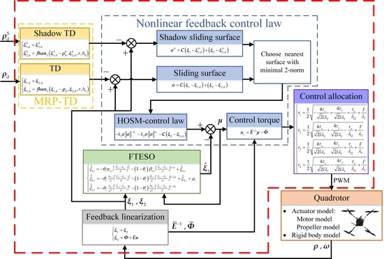
4. High-Order Sliding Mode-Based Fixed-Time Active Disturbance Rejection Control (FTADRC)

The FTADRC scheme is designed within the traditional ADRC structure based on the feedback-linearization technique. A schematic block diagram of the proposed FTADRC scheme for quadrotor attitude control is shown in Figure 7. The attitude control scheme consists of five parts:

• Feedback linearization for regularizing the attitude dynamic model;
• Fixed-time extended state observer (FTESO) for observing the unknown disturbances accurately;
• MRP-TD for tracking the differential of input attitude described by MRP;
• Non-linear feedback control law for driving the orientation of quadrotor to track the desired attitude timely;
• Control allocation for generating pulse-width modulation (PWM) signals for motors.

4.1. Feedback Linearization

We remove the gyroscopic effect and reactionary torque related to the rotor speed in the attitude dynamic equations and treat them as part of the unknown disturbance. A six-dimensional system is defined with state vector $\mathit{x}={\left[{\rho }_1,{\rho }_2,{\rho }_3,{\omega }_{\mathrm{x}},{\omega }_{\mathrm{y}},{\omega }_{\mathrm{z}}\right]}^{\mathrm{T}}$, input vector $\mathit{u}={\left[{\tau }_{\mathrm{x}},{\tau }_{\mathrm{y}},{\tau }_{\mathrm{z}}\right]}^{\mathrm{T}}$ and measurable output vector $\mathit{y}={\left[y_1,y_2,y_3\right]}^{\mathrm{T}}$. A non-linear system is achieved according to the attitude model in Equation (3).

$$\begin{array}{l}\underset{\dot{\mathit{x}}}{\underbrace{\left[\begin{array}{c}{\dot{\rho }}_1\\ {\dot{\rho }}_2\\ {\dot{\rho }}_3\\ {\dot{\omega }}_{\mathrm{x}}\\ {\dot{\omega }}_{\mathrm{y}}\\ {\dot{\omega }}_{\mathrm{z}}\end{array}\right]}}=\underset{\mathit{f}(\mathit{x})}{\underbrace{\left[\begin{array}{c}\frac{1}{4}{\omega }_{\mathrm{x}}({\rho }_1^2-{\rho }_2^2-{\rho }_3^2+1)+\frac{1}{2}{\omega }_{\mathrm{y}}({\rho }_1{\rho }_2-{\rho }_3)+\frac{1}{2}{\omega }_{\mathrm{z}}({\rho }_1{\rho }_3+{\rho }_2)\\ \frac{1}{4}{\omega }_{\mathrm{y}}({\rho }_2^2-{\rho }_1^2-{\rho }_3^2+1)+\frac{1}{2}{\omega }_{\mathrm{x}}({\rho }_1{\rho }_2+{\rho }_3)+\frac{1}{2}{\omega }_{\mathrm{z}}({\rho }_2{\rho }_3-{\rho }_1)\\ \frac{1}{4}{\omega }_{\mathrm{z}}({\rho }_3^2-{\rho }_1^2-{\rho }_2^2+1)+\frac{1}{2}{\omega }_{\mathrm{x}}({\rho }_1{\rho }_3-{\rho }_2)+\frac{1}{2}{\omega }_{\mathrm{y}}({\rho }_2{\rho }_3+{\rho }_1)\\ (I_{\mathrm{y}}-I_{\mathrm{z}}){\omega }_{\mathrm{y}}{\omega }_{\mathrm{z}}/I_{\mathrm{x}}\\ (I_{\mathrm{z}}-I_{\mathrm{x}}){\omega }_{\mathrm{x}}{\omega }_{\mathrm{z}}/I_{\mathrm{y}}\\ (I_{\mathrm{x}}-I_{\mathrm{y}}){\omega }_{\mathrm{x}}{\omega }_{\mathrm{y}}/I_{\mathrm{z}}\end{array}\right]}}+\underset{\mathit{g}}{\underbrace{\left[\begin{array}{ccc}0& 0& 0\\ 0& 0& 0\\ 0& 0& 0\\ \frac{1}{I_{\mathrm{x}}}& 0& 0\\ 0& \frac{1}{I_{\mathrm{y}}}& 0\\ 0& 0& \frac{1}{I_{\mathrm{z}}}\end{array}\right]}}\underset{\mathit{u}}{\underbrace{\left[\begin{array}{c}{\tau }_{\mathrm{x}}\\ {\tau }_{\mathrm{y}}\\ {\tau }_{\mathrm{z}}\end{array}\right]}}\\ \underset{\mathit{y}}{\underbrace{\left[\begin{array}{c}{y}_1\\ y_2\\ y_3\end{array}\right]}}=\underset{\mathit{h}(\mathit{x})}{\underbrace{\left[\begin{array}{c}{\rho }_1\\ {\rho }_2\\ {\rho }_3\end{array}\right]}}\end{array}$$

(15)

The Lie derivative and k-th Lie derivative of function $h_i(\mathit{x})$ with respect to a vector-valued function $\mathit{f}(\mathit{x})$ are defined as follows:

$$\begin{array}{l}{L}_{\mathrm{f}}{h}_i(\mathit{x})={\displaystyle \sum _{j=1}^6\frac{\partial h_i(\mathit{x})}{\partial x_j}{f}_j(\mathit{x})}\\ L_{\mathrm{f}}^k{h}_i(\mathit{x})=L_{\mathrm{f}}(L_{\mathrm{f}}^{k-1}{h}_i(\mathit{x}))\end{array}$$

(16)

A 3 × 3 matrix $\mathit{E}(\mathit{x})$ is constructed with the Lie derivatives $L_{{\mathrm{g}}_j}{L}_{\mathrm{f}}{h}_i(\mathit{x}),(i\in \left[1,3\right],j\in \left[1,3\right])$:

$$\mathit{E}(\mathit{x})=\left[\begin{array}{ccc}{L}_{{\mathrm{g}}_1}{L}_{\mathrm{f}}{h}_1(\mathit{x})& L_{{\mathrm{g}}_2}{L}_{\mathrm{f}}{h}_1(\mathit{x})& L_{{\mathrm{g}}_3}{L}_{\mathrm{f}}{h}_1(\mathit{x})\\ L_{{\mathrm{g}}_1}{L}_{\mathrm{f}}{h}_2(\mathit{x})& L_{{\mathrm{g}}_2}{L}_{\mathrm{f}}{h}_2(\mathit{x})& L_{{\mathrm{g}}_3}{L}_{\mathrm{f}}{h}_2(\mathit{x})\\ L_{{\mathrm{g}}_1}{L}_{\mathrm{f}}{h}_3(\mathit{x})& L_{{\mathrm{g}}_2}{L}_{\mathrm{f}}{h}_3(\mathit{x})& L_{{\mathrm{g}}_3}{L}_{\mathrm{f}}{h}_3(\mathit{x})\end{array}\right]$$

(17)

Substituting functions of (15) into $\mathit{E}(\mathit{x})$ yields:

$$\mathit{E}(\mathit{x})=\left[\begin{array}{ccc}\frac{{\rho }_1^2-{\rho }_2^2-{\rho }_3^2+1}{4I_{\mathrm{x}}}& \frac{{\rho }_1{\rho }_2-{\rho }_3}{2I_{\mathrm{y}}}& \frac{{\rho }_1{\rho }_3+{\rho }_2}{2I_{\mathrm{z}}}\\ \frac{{\rho }_1{\rho }_2+{\rho }_3}{2I_{\mathrm{x}}}& \frac{{\rho }_2^2-{\rho }_1^2-{\rho }_3^2+1}{4I_{\mathrm{y}}}& \frac{{\rho }_2{\rho }_3-{\rho }_1}{2I_{\mathrm{z}}}\\ \frac{{\rho }_1{\rho }_3-{\rho }_2}{2I_{\mathrm{x}}}& \frac{{\rho }_2{\rho }_3+{\rho }_1}{2I_{\mathrm{y}}}& \frac{{\rho }_3^2-{\rho }_1^2-{\rho }_2^2+1}{4I_{\mathrm{z}}}\end{array}\right]$$

(18)

with a determinant of:

$$\left|\mathit{E}(\mathit{x})\right|=\frac{{({\rho }_1^2+{\rho }_2^2+{\rho }_3^2+1)}^3}{64I_x{I}_y{I}_z}$$

(19)

Obviously $\left|\mathit{E}(\mathit{x})\right|>0$ holds for all $\mathit{\rho }\in {ℝ}^3$. Therefore, $\mathit{E}(\mathit{x})$ is non-singular. The relative degree vector of system (15) is $\mathit{r}={\left[2,2,2\right]}^{\mathrm{T}}$. System (15) can be transformed into a regular form.

$$\left[\begin{array}{c}{\ddot{y}}_1\\ {\ddot{y}}_2\\ {\ddot{y}}_3\end{array}\right]=\underset{\mathit{Ф}(\mathit{x})}{\underbrace{\left[\begin{array}{c}{L}_{\mathrm{f}}^2{h}_1(\mathit{x})\\ L_{\mathrm{f}}^2{h}_2(\mathit{x})\\ L_{\mathrm{f}}^2{h}_3(\mathit{x})\end{array}\right]}}+\mathit{E}(\mathit{x})\mathit{u}$$

(20)

The formula of a three-dimensional vector $\mathit{Ф}(\mathit{x})$ is in Appendix A. Defining a new six-dimensional state vector $\mathit{\xi }={\left[{\mathit{\xi }}_1{}^{\mathrm{T}},{\mathit{\xi }}_2{}^{\mathrm{T}}\right]}^{\mathrm{T}}={\left[{\rho }_1,{\rho }_2,{\rho }_3,{\dot{\rho }}_1,{\dot{\rho }}_2,{\dot{\rho }}_3\right]}^{\mathrm{T}}$, a new state equation is derived from (20).

$$\{\begin{array}{l}{\dot{\mathit{\xi }}}_1={\mathit{\xi }}_2\\ {\dot{\mathit{\xi }}}_2=\mathit{Ф}+\mathit{E}\mathit{u}\end{array}$$

(21)

where $\mathit{Ф}$ and $\mathit{E}$ are determined by the system model parameters. We divide them into the nominal parts $\overline{\mathit{Ф}}$, $\overline{\mathit{E}}$ and the uncertain parts $\Delta \mathit{Ф}$, $\Delta \mathit{E}$. The input torque $\mathit{u}$ is divided into the control torque ${\mathit{u}}_{\mathrm{c}}$ and the unknown disturbance torque $\Delta \mathit{u}$. $\mathit{Ф}$, $\mathit{E}$ and $\mathit{u}$ are rewritten in the following format.

$$\{\begin{array}{l}\mathit{Ф}=\overline{\mathit{Ф}}+\Delta \mathit{Ф}\\ \mathit{E}=\overline{\mathit{E}}+\Delta \mathit{E}\\ \mathit{u}={\mathit{u}}_{\mathrm{c}}+\Delta \mathit{u}\end{array}$$

(22)

Substituting (22) into (21) yields:

$$\{\begin{array}{l}{\dot{\mathit{\xi }}}_1={\mathit{\xi }}_2\\ {\dot{\mathit{\xi }}}_2=(\overline{\mathit{Ф}}+\overline{\mathit{E}}{\mathit{u}}_{\mathrm{c}})+(\Delta \mathit{Ф}+\Delta \mathit{E}{\mathit{u}}_{\mathrm{c}}+\mathit{E}\Delta \mathit{u})\end{array}$$

(23)

Define an auxiliary input vector $\mathit{\mu }$ and a lumped disturbance vector $\Delta \mathit{\mu }$ as follows:

$$\{\begin{array}{l}\mathit{\mu }=\overline{\mathit{Ф}}+\overline{\mathit{E}}{\mathit{u}}_{\mathrm{c}}\\ \Delta \mathit{\mu }=\Delta \mathit{Ф}+\Delta \mathit{E}{\mathit{u}}_{\mathrm{c}}+\mathit{E}\Delta \mathit{u}\end{array}$$

(24)

Substituting (24) into (23) yields:

$$\{\begin{array}{l}{\dot{\mathit{\xi }}}_1={\mathit{\xi }}_2\\ {\dot{\mathit{\xi }}}_2=\mathit{\mu }+\Delta \mathit{\mu }\end{array}$$

(25)

4.2. Fixed-Time Third-Order Sliding Mode Observer-Based Extended State Observer (ESO)

According to (24), the equivalent disturbance torque $\Delta \mathit{\tau }$ is related to $\Delta \mathit{\mu }$ in the format:

$$\Delta \mathit{\tau }={\overline{\mathit{E}}}^{-1}\Delta \mathit{\mu }$$

(26)

Since $\overline{\mathit{E}}$ is a non-singular matrix, the estimation of $\Delta \mathit{\tau }$ is equivalent to the estimation of $\Delta \mathit{\mu }$. Augment $\Delta \mathit{\mu }$ as an extended state ${\mathit{\xi }}_3=\Delta \mathit{\mu }$, the reconstructed linear system is rewritten as:

$$\{\begin{array}{l}{\dot{\mathit{\xi }}}_1={\mathit{\xi }}_2\\ {\dot{\mathit{\xi }}}_2={\mathit{\xi }}_3+\mathit{\mu }\\ {\dot{\mathit{\xi }}}_3=\mathit{\zeta }\end{array}$$

(27)

where $\mathit{\zeta }$ is the derivative of ${\mathit{\xi }}_3$. Assume that each element of $\mathit{\zeta }$ is bounded.

$${\zeta }_i\in \left[-L,L\right]\hspace{0.17em},\hspace{0.17em}i=1,2,3$$

(28)

The elements in a 3-dimensional vector ${\mathit{\xi }}_1$, ${\mathit{\xi }}_2$ and ${\mathit{\xi }}_3$ are independent of each other. Motivated by [31], a fixed-time convergent extended state observer (FTESO) for each element i (I = 1,2,3) is designed as:

$$\begin{array}{l}{\dot{\widehat{\xi }}}_{1,i}=-{\theta }_i{\alpha }_{1,i}{\lceil \frac{{\widehat{\xi }}_{1,i}-{\xi }_{1,i}}{\delta }\rfloor }^{\frac{2}{3}}-(1-{\theta }_i){\beta }_{1,i}{\lceil \frac{{\widehat{\xi }}_{1,i}-{\xi }_{1,i}}{\delta }\rfloor }^{1+\epsilon }+{\widehat{\xi }}_{2,i}\\ {\dot{\widehat{\xi }}}_{2,i}=-{\theta }_i\frac{{\alpha }_{2,i}}{\delta }{\lceil \frac{{\widehat{\xi }}_{1,i}-{\xi }_{1,i}}{\delta }\rfloor }^{\frac{1}{3}}-(1-{\theta }_i)\frac{{\beta }_{2,i}}{\delta }{\lceil \frac{{\widehat{\xi }}_{1,i}-{\xi }_{1,i}}{\delta }\rfloor }^{1+2\epsilon }+{\widehat{\xi }}_{3,i}+{\mu }_i\\ {\dot{\widehat{\xi }}}_{3,i}=-{\theta }_i\frac{{\alpha }_{3,i}}{{\delta }^2}{\lceil \frac{{\widehat{\xi }}_{1,i}-{\xi }_{1,i}}{\delta }\rfloor }^0-(1-{\theta }_i)\frac{{\beta }_{3,i}}{{\delta }^2}{\lceil \frac{{\widehat{\xi }}_{1,i}-{\xi }_{1,i}}{\delta }\rfloor }^{1+3\epsilon }\\ {\theta }_i=\{\begin{array}{l}0\hspace{0.17em}\hspace{0.17em},\hspace{0.17em}\hspace{0.17em}{\widehat{\xi }}_{1,i}-{\xi }_{1,i}>\delta \\ 1\hspace{0.17em}\hspace{0.17em},\hspace{0.17em}\hspace{0.17em}{\widehat{\xi }}_{1,i}-{\xi }_{1,i}\le \delta \end{array}\end{array}$$

(29)

where ${\widehat{\xi }}_{1,i}$, ${\widehat{\xi }}_{2,i}$ and ${\widehat{\xi }}_{3,i}$ are the estimation of ${\xi }_{1,i}$. ${\xi }_{2,i}$ and ${\xi }_{3,i}$ respectively. $\delta >0$ is used to scale the estimation error. Function ${\lceil x\rfloor }^k={\left|x\right|}^k\mathrm{sign}(x)$, $\mathrm{sign}(·)$ represents the signum function. $\epsilon >0$ is chosen small enough. ${\theta }_i$ is used to switch between two different exponential functions. ${\alpha }_{j,i}\hspace{0.17em}(j=1,2,3)$ are selected based on the boundary value $L$ using the formulas for the HOSM differentiator in [28]. ${\beta }_{j,i}\hspace{0.17em}(j=1,2,3)$ are selected such that the following matrix is Hurwitz as suggested by [31].

$$\mathit{A}=\left[\begin{array}{ccc}-{\beta }_{1,i}& 1& 0\\ -{\beta }_{2,i}& 0& 1\\ -{\beta }_{3,i}& 0& 0\end{array}\right]$$

(30)

There are two major improvements between the above observer with the differentiators used in [31,32].

1. The switching is conducted according to the estimation error instead of an arbitrary fixed time.

2. The estimation error ${\widehat{\xi }}_{1,i}-{\xi }_{1,i}$ is scaled with $1/\delta$.

The switching structure of the observer takes advantage of dealing with different estimation errors with different exponential functions. The function with exponential larger than 1 is more efficient with larger errors, while the function with exponential smaller than 1 is more efficient with smaller errors. So, we use a switch mechanism controlled by estimation errors to make full use of different exponential functions. The scaling factor is used to adjust flexibly the estimation errors for better performance.

Theorem 1.

Suppose that${\mathit{\xi }}_1$and$\mathit{\mu }$are available in real time. FTESO (29) converges to the true extended states${\xi }_{1,i}$,${\xi }_{2,i}$and${\xi }_{3,i}$in a fixed time with the parameters chosen according to preceding rules.

Proof of Theorem 1.

Define the following notations for observation errors.

$$\{\begin{array}{l}\Delta {\xi }_{1,i}={\widehat{\xi }}_{1,i}-{\xi }_{1,i}\\ \Delta {\xi }_{2,i}={\widehat{\xi }}_{2,i}-{\xi }_{2,i}\\ \Delta {\xi }_{3,i}={\widehat{\xi }}_{3,i}-{\xi }_{3,i}\end{array}$$

(31)

Differentiating $\Delta {\xi }_{1,i}$, $\Delta {\xi }_{2,i}$ and $\Delta {\xi }_{3,i}$, one can obtain:

$$\{\begin{array}{l}\Delta {\dot{\xi }}_{1,i}=-{\theta }_i{\alpha }_{1,i}{\lceil \frac{{\widehat{\xi }}_{1,i}-{\xi }_{1,i}}{\delta }\rfloor }^{\frac{2}{3}}-(1-{\theta }_i){\beta }_{1,i}{\lceil \frac{{\widehat{\xi }}_{1,i}-{\xi }_{1,i}}{\delta }\rfloor }^{1+\epsilon }+\Delta {\widehat{\xi }}_{2,i}\\ \Delta {\dot{\xi }}_{2,i}=-{\theta }_i\frac{{\alpha }_{2,i}}{\delta }{\lceil \frac{{\widehat{\xi }}_{1,i}-{\xi }_{1,i}}{\delta }\rfloor }^{\frac{1}{3}}-(1-{\theta }_i)\frac{{\beta }_{2,i}}{\delta }{\lceil \frac{{\widehat{\xi }}_{1,i}-{\xi }_{1,i}}{\delta }\rfloor }^{1+2\epsilon }+\Delta {\widehat{\xi }}_{3,i}\\ \Delta {\dot{\xi }}_{3,i}=-{\theta }_i\frac{{\alpha }_{3,i}}{{\delta }^2}{\lceil \frac{{\widehat{\xi }}_{1,i}-{\xi }_{1,i}}{\delta }\rfloor }^0-(1-{\theta }_i)\frac{{\beta }_{3,i}}{{\delta }^2}{\lceil \frac{{\widehat{\xi }}_{1,i}-{\xi }_{1,i}}{\delta }\rfloor }^{1+3\epsilon }-{\zeta }_i\end{array}$$

(32)

Define:

$$\{\begin{array}{l}{\eta }_{1,i}=\Delta {\xi }_{1,i}(\delta t)/\delta \\ {\eta }_{2,i}=\Delta {\xi }_{2,i}(\delta t)\\ {\eta }_{3,i}=\delta \Delta {\xi }_{3,i}(\delta t)\end{array}$$

(33)

Substituting (33) into (32) yields:

$$\{\begin{array}{l}{\dot{\eta }}_{1,i}=-{\theta }_i{\alpha }_{1,i}{\lceil {\eta }_{1,i}\rfloor }^{\frac{2}{3}}-(1-{\theta }_i){\beta }_{1,i}{\lceil {\eta }_{1,i}\rfloor }^{1+\epsilon }+\Delta {\widehat{\xi }}_{2,i}\\ {\dot{\eta }}_{2,i}=-{\theta }_i{\alpha }_{2,i}{\lceil {\eta }_{1,i}\rfloor }^{\frac{1}{3}}-(1-{\theta }_i){\beta }_{2,i}{\lceil {\xi }_{1,i}\rfloor }^{1+2\epsilon }+\Delta {\widehat{\xi }}_{3,i}\\ {\dot{\xi }}_{3,i}=-{\theta }_i{\alpha }_{3,i}{\lceil {\xi }_{1,i}\rfloor }^0-(1-{\theta }_i){\beta }_{3,i}{\lceil {\xi }_{1,i}\rfloor }^{1+3\epsilon }-{\delta }^2{\zeta }_i\end{array}$$

(34)

According to Theorem 1 in [31], (34) converges to a 3-sliding surface $S=\left\{{\eta }_{1,i}=0,{\eta }_{2,i}=0,{\eta }_{3,i}=0\right\}$ in a fixed time $T$. Therefore, (29) converges to the true extended states ${\xi }_{1,i}$, ${\xi }_{2,i}$ and ${\xi }_{3,i}$ in a fixed time $T/\delta$. This complete the proof. □

4.3. Tracking Differentiator

The tracking differentiator for the desired attitude ${\mathit{\rho }}_{\mathrm{d}}={\left[{\rho }_{1,\mathrm{d}},{\rho }_{2,\mathrm{d}},{\rho }_{3,\mathrm{d}}\right]}^{\mathrm{T}}$ based on the above feedback linearization model is obtained by directly applying the TD in the classical ADRC structure.

$$\{\begin{array}{l}{\dot{\mathit{\xi }}}_{1,\mathrm{d}}={\mathit{\xi }}_{2,\mathrm{d}}\\ {\dot{\mathit{\xi }}}_{2,\mathrm{d}}=\mathit{f}\mathit{h}\mathit{a}{\mathit{n}}_3({\mathit{\xi }}_{1,\mathrm{d}}-{\mathit{\rho }}_{\mathrm{d}},{\mathit{\xi }}_{2,\mathrm{d}},r,h_0)\end{array}$$

(35)

where function $\mathit{f}\mathit{h}\mathit{a}{\mathit{n}}_3$ is the vector version of tracking function fhan in [21]. It performs function fhan for each element of the 3-D vectors. The above tracking differentiator outputs the desired linearized states ${\mathit{\xi }}_{1,\mathrm{d}}$ and ${\mathit{\xi }}_{2,\mathrm{d}}$. Considering the multi-solution characteristic of MRP in describing rotation, the shadow tracking differentiator for ${\mathit{\rho }}_{\mathrm{d}}^{\mathrm{S}}$ should also be constructed as follows.

$$\{\begin{array}{l}{\dot{\mathit{\xi }}}_{1,\mathrm{d}}^{\mathrm{S}}={\mathit{\xi }}_{2,\mathrm{d}}^{\mathrm{S}}\\ {\dot{\mathit{\xi }}}_{2,\mathrm{d}}^{\mathrm{S}}=\mathit{f}\mathit{h}\mathit{a}{\mathit{n}}_3({\mathit{\xi }}_{1,\mathrm{d}}^{\mathrm{S}}-{\mathit{\rho }}_{\mathrm{d}}^{\mathrm{S}},{\mathit{\xi }}_{2,\mathrm{d}}^{\mathrm{S}},r,h_0)\end{array}$$

(36)

4.4. Multivariable High-Order Sliding Mode (HOSM)-Based Fixed-Time Non-Linear Feedback Law

Define the sliding surface and shadow sliding surface:

$$\begin{array}{l}\mathit{\sigma }=\mathit{C}({\mathit{\xi }}_1-{\mathit{\xi }}_{1,\mathrm{d}})+({\mathit{\xi }}_2-{\mathit{\xi }}_{2,\mathrm{d}})\\ {\mathit{\sigma }}^{\mathrm{S}}=\mathit{C}({\mathit{\xi }}_1-{\mathit{\xi }}_{1,\mathrm{d}}^{\mathrm{S}})+({\mathit{\xi }}_2-{\mathit{\xi }}_{2,\mathrm{d}}^{\mathrm{S}})\end{array}$$

(37)

where $\mathit{C}$ is a 3 × 3 diagonal matrix with positive elements of main diagonal. For tracking the desired attitude described by the MRP set $\left\{{\mathit{\rho }}_{\mathrm{d}},{\mathit{\rho }}_{\mathrm{d}}^{\mathrm{S}}\right\}$, there are two candidate sliding mode surfaces to approach. We force the quadrotor moving towards the “nearby candidate” in $\left\{\mathit{\sigma },{\mathit{\sigma }}^{\mathrm{S}}\right\}$ with minimal 2-norm. Without loss of generality, the fixed-time feedback law is designed and analyzed for $\mathit{\sigma }$ in the following.

Differentiating $\mathit{\sigma }$ and substituting (25) into the expression of $\dot{\mathit{\sigma }}$, one can obtain:

$$\dot{\mathit{\sigma }}=\mathit{C}({\mathit{\xi }}_2-{\mathit{\xi }}_{2,\mathrm{d}})+\mathit{\mu }+\Delta \mathit{\mu }$$

(38)

Inspired by [39], we use 2-norm of the 3-dimension vector $\mathit{\sigma }$ to apply the high-order sliding mode algorithm on the above multivariable system. A fixed-time second-order sliding mode control law with disturbance rejection is designed as:

$$\mathit{\mu }=-k_1\mathit{\sigma }{\Vert \mathit{\sigma }\Vert }^{-p_1}-k_2\mathit{\sigma }{\Vert \mathit{\sigma }\Vert }^{p_2}-\mathit{C}({\mathit{\xi }}_2-{\mathit{\xi }}_{2,\mathrm{d}})-{\widehat{\mathit{\xi }}}_3$$

(39)

where $k_1>0$, $k_2>0$, $0<p_1<1$, $0<p_2<1$, and the notation $\Vert \mathit{\sigma }\Vert$ represents 2-norm of vector $\mathit{\sigma }$. According to Theorem 1, ${\widehat{\mathit{\xi }}}_3$ becomes equal to $\Delta \mathit{\mu }$ in a fixed time. Substituting (39) into (38), the close-loop dynamic equation of $\mathit{\sigma }$ can be obtained.

$$\dot{\mathit{\sigma }}=-k_1\mathit{\sigma }{\Vert \mathit{\sigma }\Vert }^{-p_1}-k_2\mathit{\sigma }{\Vert \mathit{\sigma }\Vert }^{p_2}$$

(40)

Theorem 2.

Consider the closed-loop system (40), the sliding variable$\mathit{\sigma }$and its derivative$\dot{\mathit{\sigma }}$reach the origin in fixed time.

Proof of Theorem 2.

Given (40), the 3-dimension vectors $\dot{\mathit{\sigma }}$ and $\mathit{\sigma }$ are parallel in opposite directions. That means the direction of $\mathit{\sigma }$ does not change with time, and the following equation holds.

$$\Vert \dot{\mathit{\sigma }}\Vert =-\frac{d\Vert \mathit{\sigma }\Vert }{dt}$$

(41)

Substituting (40) into (41) yields:

$$\frac{d\Vert \mathit{\sigma }\Vert }{dt}=-(k_1{\Vert \mathit{\sigma }\Vert }^{-p_1}+k_2{\Vert \mathit{\sigma }\Vert }^{p_2})\Vert \mathit{\sigma }\Vert =-k_1{\Vert \mathit{\sigma }\Vert }^{1-p_1}-k_2{\Vert \mathit{\sigma }\Vert }^{1+p_2}$$

(42)

When the initial value of the system satisfies the inequation $\Vert \mathit{\sigma }(0)\Vert >1$, according to the above equation, one can obtain:

$$\frac{d\Vert \mathit{\sigma }\Vert }{dt}<-k_2{\Vert \mathit{\sigma }\Vert }^{1+p_2}$$

(43)

Inequation (43) can be rewritten as:

$$\frac{d\Vert \mathit{\sigma }\Vert }{{\Vert \mathit{\sigma }\Vert }^{1+p_2}}<-k_{2}dt$$

(44)

Denote the time consumed for $\Vert \mathit{\sigma }(t)\Vert$ reducing from $\Vert \mathit{\sigma }(0)\Vert$ to 1 to $T_1$, i.e., $\Vert \mathit{\sigma }(T_1)\Vert =1$. Integrate Equation (44), and it can be found that $T_1$ is bounded by a fixed value that is independent of initial value $\sigma (0)$.

$$T_1<\frac{1}{k_2{p}_2}$$

(45)

After the system state reaching $\Vert \mathit{\sigma }\Vert =1$ in time $T_1$, according to (42), one can obtain:

$$\frac{d\Vert \mathit{\sigma }\Vert }{dt}<-k_1{\Vert \mathit{\sigma }\Vert }^{1-p_1}$$

(46)

Denote the time consumed for $\Vert \mathit{\sigma }(t)\Vert$ reducing from 1 to 0 to $T_2$, i.e., $\Vert \mathit{\sigma }(T_1+T_2)\Vert =0$. Integrate Equation (46), and it can be concluded that if $\Vert \mathit{\sigma }(T_1)\Vert$ is in range (0,1], $T_2$ is bounded by a fixed value.

$$T_2<\frac{1}{k_1{p}_1}$$

(47)

For a 3-dimensional vector $\mathit{\sigma }$, $\Vert \mathit{\sigma }\Vert =0\iff \sigma =0$. According to Equation (40), $\dot{\mathit{\sigma }}=0$ when $\mathit{\sigma }=0$. This completes the proof. □

The control torque is calculated according to the first equation in (24).

$${\mathit{u}}_{\mathrm{c}}={\overline{\mathit{E}}}^{-1}\mathit{\mu }-\overline{\mathit{Ф}}$$

(48)

The feedback law (39) performs exponential functions on the 2-norm of $\mathit{\sigma }$ instead of three Euler angles used in [15]. In this way, the exponential functions-related computation is reduced. This characteristic is helpful when using a low-cost advanced RISC (reduced instruction set computing) machine (ARM) microprocessor that is ineffective to nonlinear functions such as exponential, trigonometric and inverse trigonometric functions.

By means of input–output feedback linearization, the non-linear attitude system is transformed into a linear system and the parameters in the observer and controller are adjusted in a standard way [28]. More importantly, the matrix B for tuning the disturbance estimation and compensation in traditional ADRC [21] is a model-related parameter even though the whole method is independent of the type of system function. This means the parameter is hard to tune in attitude control of quadrotor that the control torque is not generated directly by the controller output. The HOSM-based FTESO and non-linear feedback law are constructed based on the equivalent linear model, such that the observer and the controller are completely independent without common parameters and can be adjusted individually. In conclusion, the proposed FTADRC method is tuned more easily than the traditional ADRC method.

4.5. Non-Linear Control Allocation

The control torque is allocated to four actuators according to the actuator models. After the motors reach the steady state, the PWM signals outputted by the controller are proportional to the rotor speeds. Given the quadratic dependence of thrust and torque upon rotor speed, a simple nonlinear control allocation method is used in this paper.

$$\{\begin{array}{l}{r}_1=\frac{1}{2}\sqrt{-\frac{2{\tau }_{\mathrm{x}}}{\sqrt{2}l{\lambda }_{\mathrm{T}}}+\frac{2{\tau }_{\mathrm{y}}}{\sqrt{2}l{\lambda }_{\mathrm{T}}}+\frac{{\tau }_{\mathrm{z}}}{{\lambda }_{\mathrm{Q}}}+\frac{F}{{\lambda }_{\mathrm{T}}}}\\ r_2=\frac{1}{2}\sqrt{\frac{2{\tau }_{\mathrm{x}}}{\sqrt{2}l{\lambda }_{\mathrm{T}}}+\frac{2{\tau }_{\mathrm{y}}}{\sqrt{2}l{\lambda }_{\mathrm{T}}}-\frac{{\tau }_{\mathrm{z}}}{{\lambda }_{\mathrm{Q}}}+\frac{F}{{\lambda }_{\mathrm{T}}}}\\ r_3=\frac{1}{2}\sqrt{\frac{2{\tau }_{\mathrm{x}}}{\sqrt{2}l{\lambda }_{\mathrm{T}}}-\frac{2{\tau }_{\mathrm{y}}}{\sqrt{2}l{\lambda }_{\mathrm{T}}}+\frac{{\tau }_{\mathrm{z}}}{{\lambda }_{\mathrm{Q}}}+\frac{F}{{\lambda }_{\mathrm{T}}}}\\ r_4=\frac{1}{2}\sqrt{-\frac{2{\tau }_{\mathrm{x}}}{\sqrt{2}l{\lambda }_{\mathrm{T}}}-\frac{2{\tau }_{\mathrm{y}}}{\sqrt{2}l{\lambda }_{\mathrm{T}}}-\frac{{\tau }_{\mathrm{z}}}{{\lambda }_{\mathrm{Q}}}+\frac{F}{{\lambda }_{\mathrm{T}}}}\end{array}$$

(49)

where $r_i\hspace{0.17em},\hspace{0.17em}(i=1,2,3,4)$ represents the duty circle of PWM signal for each actuator, $l$ is the distance between the rotor and the center of mass of the quadcopter, $F$ is the whole thrust provided by remote controller, ${\lambda }_{\mathrm{T}}$ and ${\lambda }_{\mathrm{Q}}$ are the coefficients related to actuator models which can be approximately calculated with maximum thrust $T_{\max }$, maximum torque $Q_{\max }$ and maximum duty circle $r_{\max }$.

$$\begin{array}{l}{\lambda }_{\mathrm{T}}=\frac{T_{\max }}{r_{\max }{}^2}\\ {\lambda }_{\mathrm{Q}}=\frac{Q_{\max }}{r_{\max }{}^2}\end{array}$$

(50)

5. Simulation and Experimental Results

5.1. Simulation Results

A simulation model for quadrotor attitude control is built according to the mathematical models and data acquired in Section 2. The structure of the simulation model is shown in Figure 8. The controller module includes the control method to be verified. The output signals are passed into a zero-order holder before the mathematical models in order to simulate the discrete calculation on the digital processor. The model part includes the motor model, propeller aerodynamic model, and rigid body dynamic model.

The unknown wind is added into the model as external disturbance. The rotor thrust and torque are influenced by the wind speed near the propeller. As the quadrotor body is acting as an obstruction to the wind, the wind attenuates while it passes through the body. As a result, the wind speed at the upwind side is larger than the wind speed at the downwind side. The wind attenuation is related to the interaction between the quadrotor body and the wind. In this paper, the wind speed is resolved into a component $\mathit{w}$ parallel to the rotor disk and a component $\mathit{u}$ perpendicular to the rotor disk. The attenuation of $\mathit{u}$ is neglected so that $\mathit{u}$ is constant near the quadrotor body. $\mathit{w}$ decreases proportionally with the distance traveled along the quadrotor body. Figure 9 is a graphical representation of $\mathit{w}$ decreasing with its travel along the quadrotor body. The green dashed line is the component $\mathit{w}$ passing the body centroid. ${\mathit{p}}_i(i=1,2,3,4)$ represents four rotor centers. After projecting ${\mathit{p}}_i$ on the gray line, the projection point closest to the wind direction is selected as the windward point ${\mathit{p}}_{\mathrm{w}}$. The wind speed near the rotor corresponding to ${\mathit{p}}_{\mathrm{w}}$ is supposed to be $\mathit{w}$. The wind speed near other three rotors is calculated as follows:

$${\mathit{w}}_i=\max (1-{\gamma }_{\mathrm{w}}{d}_i,0)\mathit{w}$$

(51)

where ${\gamma }_{\mathrm{w}}$ is the attenuation factor, $d_i$ is the distance between rotor i with ${\mathit{p}}_{\mathrm{w}}$ along vector $\mathit{w}$.

The above wind attenuation leads to different thrust at the upwind side and downwind side and in turn generates a wind-related overturning torque which acts as the disturbance in attitude control system.

The commonly used Dryden turbulence model is used to generate random wind. The fundamental of the Dryden model is constructing a transfer function based on spectrum functions of atmospheric turbulence velocity and its gradient to convert the white noise signal to a colored noise signal. The Dryden module in aerospace toolbox of Simulink (Version 8.9, MathWorks., Natick, MA, United States, 2017) is used in this paper to generate random wind speed. The low-altitude intensity in the model is set to 10m/s. The other parameters are decided according to MIL-F-8785C standard. The wind speed along three axes of Earth coordinates framed with an altitude of 6m is shown in Figure 10.

We present the mathematical simulations of proposed FTADRC attitude control method on a quadrotor model with the parameters in

Table 3. Parameters of the quadrotor in simulations.

Parameter	Description	True Value	Nominal Value
Ix	Inertia along xb-axis	0.1 kgm2	0.05 kgm2
Iy	Inertia along yb-axis	0.1 kgm2	0.05 kgm2
Iz	Inertia along zb-axis	0.22 kgm2	0.5 kgm2
l	Distance between rotor and centroid	0.4 m	0.4 m
m	Mass	8 kg	--
Kv	Motor velocity constant	325 rpm/V	--
$R_{\mathrm{M}}$	Equivalent resistance of motor	0.26 Ω	--

. The other parameters related to propeller shape and aerodynamics are chosen as Section 2.3. The first four parameters in Table 3 are used in the controller. Practically, l is easy to measure, while the inertias are hard to obtain. So, the nominal parameters are selected as the last column.

In the simulations, the position of the quadrotor is assumed to be free from the forces that include the propeller thrust and gravity. A square wave signal with amplitude of 20°, period of 8s is used as the desired roll angle input to analyze the step response. The random wind generated by the Dryden model is added into the simulation since the 15th second in order to compare the proposed FTADRC with the traditional ADRC in the absence and presence of dynamic wind disturbance. The simulation results of two different attitude control methods are shown in Figure 11, Figure 12, Figure 13, Figure 14, Figure 15 and Figure 16.

As illustrated in Figure 11, quick convergence of the roll angle is achieved by both methods before 15 s with no disturbances because we tune the parameters of the two different controllers to achieve high-gain feedback control. With the presence of simulated dynamic wind, FTADRC tracks the desired attitude more accurately than traditional ADRC. Figure 14, Figure 15 and Figure 16 indicate that the disturbance estimation of FTESO is more precise than traditional ESO.

The sharp peaks in Figure 14, Figure 15 and Figure 16 are caused by motor inertia which is generally neglected in previous researches. The motors are not able to provide the rapidly changing control torque to follow the step input. The deviation of control torque acts as a rapidly changing disturbance which is difficult to track for both FTESO and ESO. However, the sudden disturbance vanishes quickly as the motor tracks the desired speed, and the attitude of the quadrotor is not seriously affected.

5.2. Experimental Results

In order to verify the effectiveness of the proposed FTADRC attitude control method in practical applications, we have developed a flight control unit (FCU) mainly using an STM32F103 micro-processor (STMicroelectronics, Geneva, Switzerland) and two ICM-20689 inertial measurement units (IMUs, InvenSense, San Jose, CA, United States). The angular speed and acceleration information provided by the two IMUs is averaged to generate more accurate measurements. An external HMC5983 magnetometer (Honeywell, Morris Plains, NJ, United States) is used for assisting the attitude determination process. The attitude determination algorithm in [40] is applied to the FCU providing attitude measurements. The core components including micro-processor and sensors cost less than 40 US dollars. In the experiments, the proposed fixed-time disturbance rejection control method consumes less than 1 ms on the 72 MHz ARM processor.

The experiments are conducted with a self-assembled QR450 quadrotor. The experimental setup consists of a remote controller, a ground control station (GCS) and the quadrotor with FCU onboard is shown in Figure 17. A pair of Xbee modules is used for communication between the FCU and GCS.

The quadrotor frame is made by aluminium alloy and carbon fiber to lower costs, and it has been deformed after being used for more than a year in plenty of flight tests, as shown in Figure 18. The deformations result in additional disturbances as the parameters are set ignoring them. The parameters are chosen as

Table 4. Control parameters used in the experiments.

Parameters	Nominal Value
$I_{\mathrm{x}}$	0.01 kgm2
$I_{\mathrm{y}}$	0.01 kgm2
$I_{\mathrm{z}}$	0.02 kgm2
$\mathit{C}$	diag(5,5,30)
$k_1$	70
$k_2$	10
$p_1$	0.5
$p_2$	0.5

, in which $I_{\mathrm{x}}$, $I_{\mathrm{y}}$ and $I_{\mathrm{z}}$ are estimated intuitively without precise measurement.

The experiments are conducted indoors without Global Positioning System (GPS) signals. To assure flight security, the quadrotor is controlled remotely. The external unknown disturbance is simulated in three different ways. The performance of rejecting disturbance is verified respectively in all cases.

Case 1.Eccentric mass

In this case, an iron mass block of 194 g acting as the eccentric mass is hung from the right-hand front corner of the quadrotor frame, as shown in Figure 19. The original quadrotor without the eccentric mass is 1195 g. The eccentric mass is equivalent to 16% of the original quadrotor and 64% of individual motor thrust during hovering in weight. In addition, the block waves during flight and generates time-varying disturbance. The iron block hung from a corner of the frame mainly acts as an unknown constant torque in the attitude control system. In a simple error-driven control method, the constant disturbance torque will cause an attitude bias.

The curves of the attitude angles are shown in Figure 20, Figure 21 and Figure 22, and the curves of the estimated disturbances are shown in Figure 23. The roll and pitch angles are affected by the eccentric mass and the control errors increase to about 2° in 1.5 s after the quadrotor takes off from the ground. The FTESO tracks the unknown disturbances in about 3 s with an initial value of 0. The fast-changing desired roll and pitch angles are produced by remote controller to test the controller’s performance. By estimating and attenuating the estimated disturbances, the attitude angles are tracked accurately.

Case 2.Sudden fault of a single motor

In this case, we simulate the actuator fault of motor 1 (right hand front motor) with a programed effectiveness loss of 30%, which means the output duty circle of motor 1 is multiplied by 0.7. The time of fault and recovery is controlled by a digital switch on the remote controller. As a non-redundant system, the quadrotor is sensitive to motor faults. The attitude model is uncontrollable if any of the four motors is completely disabled. So, we employ a programed motor effectiveness loss instead of a complete motor failure to model an in-flight actuator fault.

In the experiment, the fault occurs at 6.4 s and the motor recovers at 32.4 s. The curves of attitude angles are shown in Figure 24, Figure 25 and Figure 26, and the curves of estimated disturbances are shown in Figure 27. The roll angle quickly changes to 19.8°, and the pitch angle quickly changes to −14.8° as a result of the motor fault. FTESO converges to the disturbances caused by the fault and the attitude angles track the desired values after 16 s.

The recovery of the motor is also treated as an external disturbance. It can be easily known from the motor model that the acceleration of the motor is slower than the deceleration. Thus, the recovery process has less impact on the quadrotor with a bounded disturbance differential-based FTESO. The roll angle changes to −16.4°, and the pitch angle changes to 14.4° 0.4 s after the motor recovers from the fault. The disturbance estimations of FTESO approximately turn back to the values before the motor fault 5.6 s after the recovery.

Case 3.Wind and damaged propeller

In this case, we install a damaged propeller on motor 2 (left hand front motor) and use two electrical fans to generate the external wind as shown in Figure 28. We make the quadrotor hover in the wind by remote control. The average wind speed generated by the two electrical fans is around 4.5 m/s. The main purpose of this case is to show the performance of FTADRC method with common lumped disturbances in quadrotor attitude control such as wind disturbance and propeller damage. Figure 29, Figure 30, Figure 31 and Figure 32 present the experimental results of the FTADRC and conventional ADRC schemes. In each figure, panel (a) indicates the result of FTADRC, and panel (b) indicates the result of conventional ADRC.

Figure 29, Figure 30 and Figure 31 present the tracking errors of attitude angles of FTADRC and conventional ADRC control schemes. The tracking errors of roll and pitch angles using FTADRC control scheme keep below 2° with average values around 0°, while the tracking errors of roll and pitch angles using the ADRC control scheme have peak-to-peak values larger than 15° and obviously non-zero average values. Figure 32 shows disturbance estimation with FTADRC and traditional ADRC schemes. The disturbance introduced by the wind is hard to evaluate accurately because of the complicated wind dynamics related to the electrical fans. However, it still could be seen from Figure 32 that the disturbance estimation using FTADRC changes faster than that using conventional ADRC. Along with the tracking errors of attitude angles, it can be demonstrated that FTADRC responds more quickly to the external disturbances and tracks the input attitude more accurately than conventional ADRC.

6. Discussion

In the experiment with eccentric mass, the quadrotor takes off from the ground slowly so that the eccentric mass could be regard as a disturbance accumulating during take-off. Thus, its influence on attitude angles is not obvious and FTESO converges to the lumped disturbances quickly. During the flight, the attitude of the quadrotor accurately tracks the desired attitude with disturbances rejected by FTESO. This experiment together with the simulations demonstrate the stability and robustness of FTADRC in the presence of slowly varying disturbance such as dynamic wind and eccentric mass.

In the experiment with a motor fault, the disturbance caused by the fault takes effect rapidly. Strictly speaking, the differential of disturbance exceeds the bound set in FTESO, and the proposed FTADRC is not suitable for such a case theoretically. However, the results show that the attitude system of quadrotor is stabled by FTADRC except that FTESO consumes more time for convergence. Therefore, the proposed robust control scheme could be applied to the practical situations beyond the theoretical constraints.

Since the motor merely fails in flight and the centroid of mass is generally adjusted before flight, the conditions in the previous two cases are rigorous, and not normal in the practical operation of quadrotors. The last case with damaged propeller and unknown wind represents a more common operation situation of a low-cost quadrotor. In this experiment, the proposed FTADRC and conventional ADRC attitude control schemes are compared. The performance of FTADRC clearly exceeds the conventional ADRC according to the results.

7. Conclusions

In this paper, the FTADRC scheme is proposed based on a HOSM method for the attitude control of a quadrotor with unknown disturbance. The control scheme employs a fixed-time ESO for observing the lumped disturbance, and uses a multivariable fixed-time second-order sliding mode method to fast approach the sliding surface for a feedback-linearized system. Detailed mathematical models are built for simulation analysis. According to the comparative simulation and experiment results, the attitude control accuracy is improved compared with the traditional ADRC because FTESO achieves higher precision than the traditional ESO, and the control scheme is effective on a low-cost flight control unit. It can be concluded that the proposed FTADRC is robust toward dynamic wind, mass eccentricity, and motor fault. Additionally, FTADRC is practical for a low-cost quadrotor because of its high time-efficiency.

References

1. Bouabdallah, S.; Murrieri, P.; Siegwart, R. Design and control of an indoor micro quadrotor. In Proceedings of the IEEE International Conference on Robotics and Automation, New Orleans, LA, USA, 26 April–1 May; pp. 4393–4398.
2. Özbek, N.S.; Önkol, M.; Efe, M.Ö. Feedback control strategies for quadrotor-type aerial robots: A survey. Trans. Inst. Meas. Control 2016, 38, 529–554. [Google Scholar] [CrossRef]
3. Lee, H.; Kim, H.J. Trajectory tracking control of multirotors from modelling to experiments: A survey. Int. J. Control Autom. Syst. 2017, 15, 281–292. [Google Scholar] [CrossRef]
4. Tayebi, A.; McGilvray, S. Attitude stabilization of a vtol quadrotor aircraft. IEEE Trans. Control Syst. Technol. 2006, 14, 562–571. [Google Scholar] [CrossRef]
5. Mahony, R.; Kumar, V.; Corke, P. Multirotor aerial vehicles modeling, estimation, and control of quadrotor. IEEE Robot. Autom. Mag. 2012, 19, 20–32. [Google Scholar] [CrossRef]
6. Pounds, P.; Mahony, R.; Corke, P. Modelling and control of a large quadrotor robot. Control Eng. Practice 2010, 18, 691–699. [Google Scholar] [CrossRef] [Green Version]
7. Kendoul, F. Survey of advances in guidance, navigation, and control of unmanned rotorcraft systems. J. Field Robot. 2012, 29, 315–378. [Google Scholar] [CrossRef]
8. Lee, D.; Kim, H.J.; Sastry, S. Feedback linearization vs. Adaptive sliding mode control for a quadrotor helicopter. Int. J. Control Autom. Syst. 2009, 7, 419–428. [Google Scholar] [CrossRef]
9. Kim, J.; Kang, M.S.; Park, S. Accurate modeling and robust hovering control for a quad-rotor vtol aircraft. In Proceedings of the 2nd International Symposium on UAVs, Reno, NV, USA, June 2009; pp. 9–26. [Google Scholar]
10. Lyu, X.M.; Zhou, J.N.; Gu, H.W.; Li, Z.X.; Shen, S.J.; Zhang, F. Disturbance observer based hovering control of quadrotor tail-sitter vtol uavs using h-infinity synthesis. IEEE Robot. Autom. Lett. 2018, 3, 2910–2917. [Google Scholar] [CrossRef]
11. Dierks, T.; Jagannathan, S. Output feedback control of a quadrotor uav using neural networks. IEEE Trans. Neural Netw. 2010, 21, 50–66. [Google Scholar] [CrossRef] [PubMed]
12. Aboudonia, A.; El-Badawy, A.; Rashad, R. Disturbance observer-based feedback linearization control of an unmanned quadrotor helicopter. Proc. Inst. Mech. Eng. Part I: J. Syst. Control Eng. 2016, 230, 877–891. [Google Scholar] [CrossRef]
13. Aboudonia, A.; Rashad, R.; El-Badawy, A. Composite hierarchical anti-disturbance control of a quadrotor uav in the presence of matched and mismatched disturbances. J. Intell. Robot. Syst. 2018, 90, 201–216. [Google Scholar] [CrossRef]
14. Xiao, B.; Yin, S. A new disturbance attenuation control scheme for quadrotor unmanned aerial vehicles. IEEE Trans. Ind. Inform. 2017, 13, 2922–2932. [Google Scholar] [CrossRef]
15. Ahmed, N.; Chen, M. Sliding mode control for quadrotor with disturbance observer. Adv. Mech. Eng. 2018, 10, 16. [Google Scholar] [CrossRef]
16. Benallegue, A.; Mokhtari, A.; Fridman, L. High-order sliding-mode observer for a quadrotor uav. Int. J. Robust Nonlinear Control 2008, 18, 427–440. [Google Scholar] [CrossRef]
17. Besnard, L.; Shtessel, Y.B.; Landrum, B. Quadrotor vehicle control via sliding mode controller driven by sliding mode disturbance observer. J. Frankl. Inst. 2012, 349, 658–684. [Google Scholar] [CrossRef]
18. Fethalla, N.; Saad, M.; Michalska, H.; Ghommam, J. Robust observer-based dynamic sliding mode conroller for a quadrotor uav. IEEE Access 2018, 6, 45846–45859. [Google Scholar] [CrossRef]
19. Shi, D.; Wu, Z.; Chou, W. Super-twisting extended state observer and sliding mode controller for quadrotor uav attitude system in presence of wind gust and actuator faults. Electronics 2018, 7, 128. [Google Scholar] [CrossRef]
20. Shi, D.; Wu, Z.; Chou, W. Generalized extended state observer based high precision attitude control of quadrotor vehicles subject to wind disturbance. IEEE Access 2018, 6. [Google Scholar] [CrossRef]
21. Han, J. From pid to active disturbance rejection control. IEEE Trans. Ind. Electron. 2009, 56, 900–906. [Google Scholar] [CrossRef]
22. Wu, Z.-H.; Guo, B.-Z. On convergence of active disturbance rejection control for a class of uncertain stochastic nonlinear systems. Int. J. Control 2017, 1–14. [Google Scholar] [CrossRef]
23. Guo, B.Z.; Zhao, Z.L. Active Disturbance Rejection Control for Nonlinear Systems: An Introduction, 1st ed.; John Wiley & Sons: Hoboken, NJ, USA, 2017; pp. 6–9. [Google Scholar]
24. Yang, H.J.; Cheng, L.; Xia, Y.Q.; Yuan, Y. Active disturbance rejection attitude control for a dual closed-loop quadrotor under gust wind. IEEE Trans. Control Syst. Technol. 2018, 26, 1400–1405. [Google Scholar] [CrossRef]
25. Ma, D.L.; Xia, Y.Q.; Li, T.Y.; Chang, K. Active disturbance rejection and predictive control strategy for a quadrotor helicopter. IET Contr. Theory Appl. 2016, 10, 2213–2222. [Google Scholar] [CrossRef]
26. Guo, Y.; Jiang, B.; Zhang, Y. A novel robust attitude control for quadrotor aircraft subject to actuator faults and wind gusts. IEEE/CAA J. Autom. Sinica 2018, 5, 292–300. [Google Scholar] [CrossRef]
27. Levant, A. Robust exact differentiation via sliding mode technique. Automatica 1998, 34, 379–384. [Google Scholar] [CrossRef]
28. Levant, A. Higher-order sliding modes, differentiation and output-feedback control. Int. J. Control 2003, 76, 924–941. [Google Scholar] [CrossRef]
29. Basin, M.; Yu, P.; Shtessel, Y. Finite-and fixed-time differentiators utilising hosm techniques. IET Control Theory Appl. 2016, 11, 1144–1152. [Google Scholar] [CrossRef]
30. Menard, T.; Moulay, E.; Perruquetti, W. Fixed-time observer with simple gains for uncertain systems. Automatica 2017, 81, 438–446. [Google Scholar] [CrossRef] [Green Version]
31. Angulo, M.T.; Moreno, J.A.; Fridman, L. Robust exact uniformly convergent arbitrary order differentiator. Automatica 2013, 49, 2489–2495. [Google Scholar] [CrossRef]
32. Li, P.; Ma, J.; Zheng, Z. Disturbance-observer-based fixed-time second-order sliding mode control of an air-breathing hypersonic vehicle with actuator faults. Proc. Inst. Mech. Eng. Part G: J. Aerosp. Eng. 2018, 232, 344–361. [Google Scholar] [CrossRef]
33. Ni, J.; Liu, L.; Chen, M.; Liu, C. Fixed-time disturbance observer design for brunovsky system. IEEE Trans. Circuit Syst. Part 2: Express Birefs 2018, 65, 341–345. [Google Scholar] [CrossRef]
34. Yu, P.; Shtessel, Y.; Edwards, C. Continuous higher order sliding mode control with adaptation of air breathing hypersonic missile. Int. J. Adapt. Control Signal Process. 2016, 30, 1099–1117. [Google Scholar] [CrossRef] [Green Version]
35. Basin, M.V.; Yu, P.; Shtessel, Y.B. Hypersonic missile adaptive sliding mode control using finite-and fixed-time observers. IEEE Trans. Ind. Electron. 2018, 65, 930–941. [Google Scholar] [CrossRef]
36. Yu, X.; Li, P.; Zhang, Y. The design of fixed-time observer and finite-time fault-tolerant control for hypersonic gliding vehicles. IEEE Trans. Ind. Electron. 2018, 65, 4135–4144. [Google Scholar] [CrossRef]
37. Schaub, H.; Junkins, J.L. Stereographic orientation parameters for attitude dynamics: A generalization of the rodrigues parameters. J. Astron. Sci. 1996, 44, 1–19. [Google Scholar]
38. Leishman, G.J. Principles of Helicopter Aerodynamics, 2nd ed.; Cambridge university press: Cambridge, UK, 2006; pp. 55–167. [Google Scholar]
39. Basin, M.; Panathula, C.B.; Shtessel, Y. Multivariable continuous fixed-time second-order sliding mode control: Design and convergence time estimation. IET Control Theory Appl. 2016, 11, 1104–1111. [Google Scholar] [CrossRef]
40. Madgwick, S. An efficient orientation filter for inertial and inertial/magnetic sensor arrays. Report x-io Univ. Bristol 2010, 25, 113–118. [Google Scholar]
Figure 1. Definition of coordinate frames.
Electronics 07 00357 g001
Figure 2. Graphic representation of original modified Rodrigues parameter (MRP) and shadow MRP.
Electronics 07 00357 g002
Figure 3. Blade element.
Electronics 07 00357 g003
Figure 4. Tensionmeter, torquemeter and tachometer.
Electronics 07 00357 g004
Figure 5. Measurements and fitting curves. (a) Trust curve; (b) torque curve.
Electronics 07 00357 g005
Figure 6. Structure of active disturbance rejection controller for second-order system.
Electronics 07 00357 g006
Figure 7. Block diagram of the proposed fixed-time active disturbance rejection control (FTADRC) attitude control scheme.
Electronics 07 00357 g007
Figure 8. Structure of simulation model.
Electronics 07 00357 g008
Figure 9. Chart of calculating the wind speed around each propeller.
Electronics 07 00357 g009
Figure 10. Random wind speed generated by Dryden model.
Electronics 07 00357 g010
Figure 11. Curves of roll angle.
Electronics 07 00357 g011
Figure 12. Curves of pitch angle.
Electronics 07 00357 g012
Figure 13. Curves of yaw angle.
Electronics 07 00357 g013
Figure 14. Curves of observation error for Δ τ x .
Electronics 07 00357 g014
Figure 15. Curves of observation error for Δ τ y .
Electronics 07 00357 g015
Figure 16. Curves of observation error for Δ τ z .
Electronics 07 00357 g016
Figure 17. Experimental system.
Electronics 07 00357 g017
Figure 18. Deformation of quadrotor frame used in the experiments.
Electronics 07 00357 g018
Figure 19. A mass block hung from the right hand front corner is used as the eccentric mass.
Electronics 07 00357 g019
Figure 20. Curves of roll angle.
Electronics 07 00357 g020
Figure 21. Curves of pitch angle.
Electronics 07 00357 g021
Figure 22. Curves of yaw angle.
Electronics 07 00357 g022
Figure 23. Curves of disturbance estimation.
Electronics 07 00357 g023
Figure 24. Curves of roll angle.
Electronics 07 00357 g024
Figure 25. Curves of pitch angle.
Electronics 07 00357 g025
Figure 26. Curves of yaw angle.
Electronics 07 00357 g026
Figure 27. Curves of disturbance estimation.
Electronics 07 00357 g027
Figure 28. Experimental environment with wind and damaged propeller.
Electronics 07 00357 g028
Figure 29. Tracking errors of roll angle using different control schemes: (a) FTADRC; (b) conventional ADRC.
Electronics 07 00357 g029
Figure 30. Tracking errors of pitch angle using different control schemes: (a) FTADRC; (b) conventional ADRC.
Electronics 07 00357 g030
Figure 31. Tracking errors of yaw angle using different control schemes: (a) FTADRC; (b) conventional ADRC.
Electronics 07 00357 g031
Figure 32. Curves of disturbance estimation using different control schemes: (a) FTADRC; (b) conventional ADRC.
Electronics 07 00357 g032