Modeling the Hysteresis Characteristics of Transformer Core under Various Excitation Level via On-Line Measurements

Abstract

In this paper, the hysteresis characteristics of a transformer core are determined from limited on-line measured voltages and currents under certain excitations. A method for calculating the magnetization curve and hysteresis loops of the transformer core under various excitation is developed based on limited excitation conditions, and using the deep neural network, support vector regressor and the Wlodarski model. The coercivity and the amplitude of magnetic field strength of hysteresis loops can be captured with high accuracy based on this method. Then, a finite element model of the transformer core is constructed to predict the distributed magnetic flux density and the excitation current using the calculated hysteresis loops. The currents from various excitation voltages on two different transformer structures are also measured to compared with simulated currents. The outcome indicates that the overall hysteresis loops and magnetization curve of the transformer core may be useful for modeling the magnetic field and excitation current under any voltage excitation.

1. Introduction

Transformer noise has become a pressing environmental issue as population growth and energy demand increasingly result in transformer stations being in close proximity to residential areas. Effective and accurate transformer core vibration modeling will facilitate reduction of core vibration and noise generation. The transformer core vibration is produced by magnetostriction and electromagnetic forces, which are determined by the distributed magnetic field in the core structure.

Accurate prediction of the magnetic field in a transformer is a difficult task due to the complicated assembly, boundary conditions, and nonlinear properties of the material [1]. The latter resulting from the nonlinear relationship between magnetic field strength (H) and magnetic flux density (B) within the ferromagnetic core. This nonlinear relationship is described by the magnetization curve and magnetic hysteresis loops and can be measured under material aspect [2,3,4] or by considering the equivalent circuit of entire equipments [5,6,7,8,9]. Since there is no general analytical formula for the hysteresis loops and magnetization curve, several empirical equations are used to describe the nonlinear property of the hysteresis loops, including the Preisach model [10], the Jiles–Atherton model [2,11], and Wlodarski model [12,13]. The Preisach model is relatively complicated to implement for practical application and the Jiles–Atherton model requires five key parameters which are not easy to be determined [14]. Unlike these models, the Wlodarski model is simple and it captures the critical physical points like the coercivity ($H_c$) and the amplitude of magnetic field strength ($H_{amp}$) of the hysteresis loops [12,13]. It models the main magnetization curve first and expands it into the family of hysteresis loops directly dependent on $H_c$ and $H_{amp}$. Furthermore, $H_c$ and $H_{amp}$ are important for current and magnetic field simulation as they describe the loss, the time when flux changes direction and the amplitude of the maximum flux. Therefore, the Wlodarski model was selected in this paper for capturing them. Since $H_c$ and $H_{amp}$ in this model need to determined separately by experiment, the method for determining these two parameters with the on-line data was also proposed in this paper. The determination of B–H relationship is important for magnetic field simulation not only in the transformer, but also in other electric machines.

Advances in computer performance and machine learning now permit the magnetization curve and hysteresis loops to be investigated using more advanced techniques. In 2001, Mahmoud et al. used the recurrent neural network to model the dynamic magnetic hysteresis loops based on the Preisach model [15]. In 2002, Alessandro applied genetic algorithms and a fully connected neural network to generalize the Jiles–Atherton model under different frequency and the error was less than 3% [2]. The model was obtained by using a fully connected neural network to calculate parameters in Jiles–Atherton model for hysteresis loops simulation based on their experiment data. In 2007 Li used multi-layer artificial neural network to train the Preisach model and achieved an error less than 0.33% under a test with actuator PZT753-21C [6]. In 2016, Deželak et al. proposed using a neural network to detect the magnetic saturation level within the transformer core [16]. However, further extension to hysteresis loops under any excitation voltage accurately is not considered in their work. This is the constraint in the simulation of magnetic flux distribution where the major methods for obtaining hysteresis loops under different excitation level is scaling or using the predefine template, while such models are limited in reflecting the actual hysteresis behavior like the $H_c$ and the $H_{amp}$ [17,18].

In this paper, we propose to use the on-line measured voltage and current collected from operating transformers and feed them into deep neural network (DNN) [19] and support vector regressor (SVR) [20] to obtain the overall magnetization curve and hysteresis loops of transformer cores under any excitation. The magnetization curve was determined via DNN and $H_c$ and $H_{amp}$ were determined by SVR and fed into the Wlodarski model for hysteresis loops modeling. DNN is a machine learning algorithm, which is based on a large collection of neural units that loosely model the way the biological brain solves problems with large clusters of biological neurons connected by axons with multiple layers. SVR is a discriminative machine learning algorithm that is formally defined by a separating hyperplane to maximize the margin in the attribute dimensions. In order to capture the critical physical point of the hysteresis loops, the Wlodarski model was selected as the basic model due to its consideration of $H_c$ and $H_{amp}$ and it is also easy to implement. Using the calculated hysteresis loops under any voltage, finite element method (FEM) was applied to calculate the excitation current and magnetic field under different excitations. The method was verified by experimental measurement of the current from transformers under different configurations and excitation methods. It shows that the overall magnetization curve and hysteresis loops of the transformer core can be applied under different configurations and excitations for further simulation in FEM.

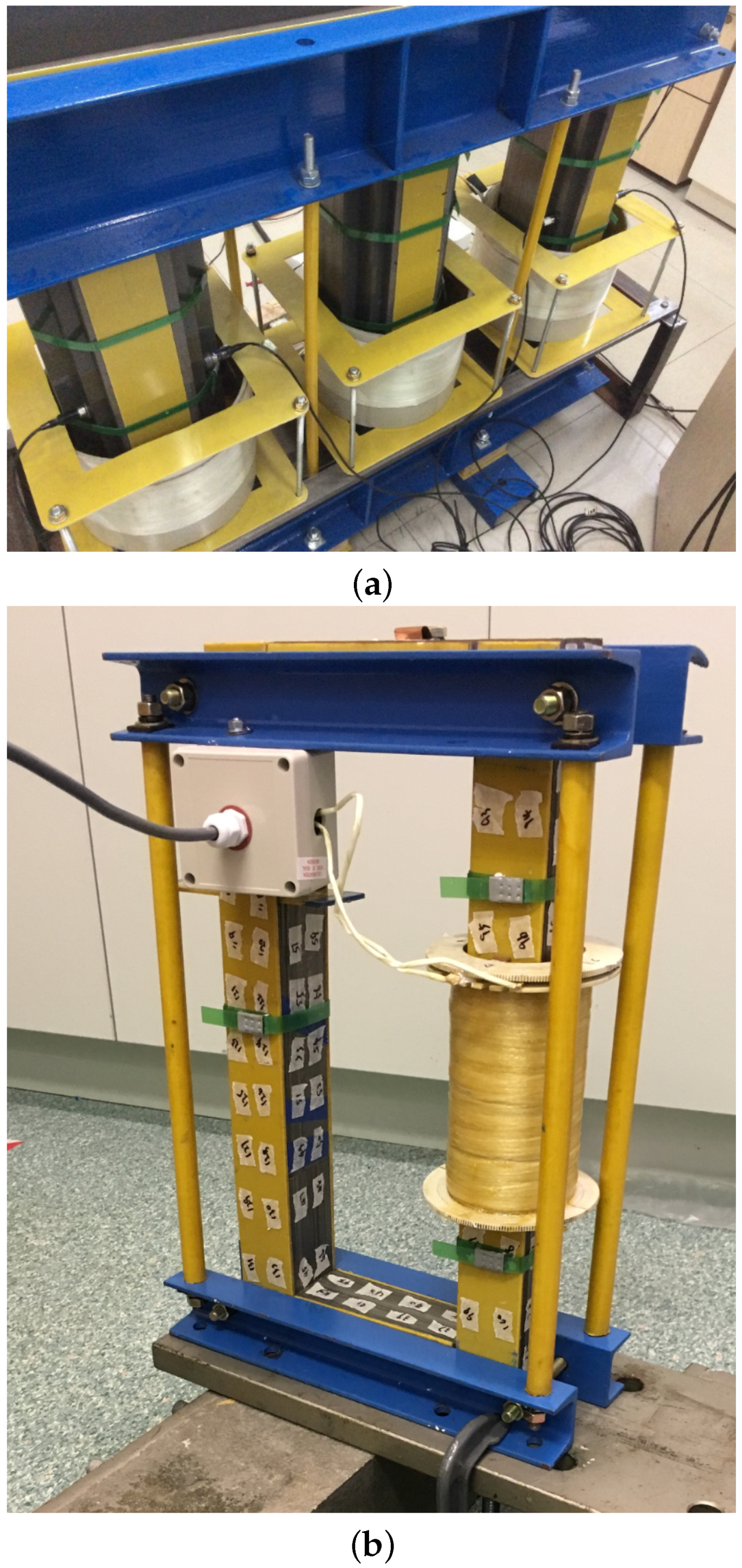
2. Materials and Methods

The overall magnetization curve and hysteresis loops under operating condition are determined by three steps: (1) reverse calculation of hysteresis loops under certain excitation based on the on-line voltage and current using the electrical circuit equation and Ampere’s circuit law; (2) from the reverse calculated hysteresis loops, $H_{amp}$, and $H_c$ under certain excitation voltage are collected. Then, DNN and SVR are used to obtain the complete magnetization curve, $H_{amp}$, and $H_c$ under any excitation voltage; and (3) applying these parameters to calculate the hysteresis loops under different excitation voltages using Wlodarski model [12].

Firstly, a family of hysteresis loops under limited excitation voltages is obtained through the on-line measured voltage and current by reverse calculation. The common V, i relationship with B and H, i.e., the Kirchhoff and ampere circuit laws are presented in Equations (1) and (2), respectively.

$$\mathbf{v}=N\frac{d(BS)}{dt}+Ri$$

(1)

$$Ni=Hl$$

(2)

where N is the number of the turns in coil, B is the magnetic flux density, $\mathit{v}$ is the excitation voltage, i is the resultant current, R is the resistance, H is the magnetic field strength and l is the length of the magnetic path. These enable one to solve for the magnetic flux density B and magnetic field strength H by measuring voltage and current resulting the magnetization curve and hysteresis loops. Based on the above reverse calculation, the proposed method can be generalised to other electric machines as long as their magnetic path can be estimated.

In this experiment, 15 pairs of on-line voltage and current were collected with sampling frequency of 10 kHz on a three-phase transformer under B-phase excitation. During the magnetization process, although different hysteresis loops will be constructed under different excitation voltage, their vertex points, corresponding to the maximum magnetic flux density and the $H_{amp}$, are always lie on the magnetization curve. Therefore, these vertex points of different pairs can be treated as samples for approaching the magnetization curve. Since one single cycle represents one hysteresis loop, 720 cycles were selected randomly from each voltage current pair where the vertex point from each cycle has small fluctuation. Therefore, 10,800 samples were obtained for training and testing.

The formulation of the magnetization curve is simulated with a three-layer DNN by training the vertex points from the hysteresis loops. The measured vertex points were divided so that 70% could be used as the training set for modeling the magnetization curve and 30% as the test set for model verification. The fully connected DNN was constructed with three layers and six, and three hidden nodes at the hidden layers with the hyperbolic tangent function as the activation function. The root mean square error (RMSE) is selected as the loss function. These are shown in These are shown in Figure 1, Equations (3)–(6), respectively.

$$a_i^1(\omega )=\frac{e^{(W_i^1{x}_n+b^1)}-e^{-(W_i^1{x}_n+b^1)}}{e^{(W_i^1{x}_n+b^1)}+e^{-(W_i^1{x}_n+b^1)}}$$

(3)

where $i=1,2,\dots ,6$, $a_i^1$ is the output of the first hidden layers and ${\mathbf{W}}^1$ is a $6\times 1$ matrix.

$$a_i^2(\omega )=\frac{e^{({\mathbf{W}}_i^2{\mathbf{a}}_i^{1,T}+b^2)}-e^{-({\mathbf{W}}_i^2{\mathbf{a}}_i^{1,T}+b^2)}}{e^{({\mathbf{W}}_i^2{\mathbf{a}}_i^{1,T}+b^2)}+e^{-({\mathbf{W}}_i^2{\mathbf{a}}_i^{1,T}+b^2)}}$$

(4)

where $i=1,2,3$, $a_i^2$ is the output of the second hidden layers, ${\mathbf{a}}_i^1=[a_1^1,a_2^1,a_3^1,a_4^1,a_5^1,a_6^1]$, ${\mathbf{W}}_i^2$ is a $1\times 6$ matrix and ${\mathbf{W}}^2$ is a $3\times 6$ matrix.

$${\hat{y}}_n(\omega )=\frac{e^{({\mathbf{W}}^3{\mathbf{a}}^{2,T}+b^3)}-e^{-({\mathbf{W}}^3{\mathbf{a}}^{2,T}+b^3)}}{e^{({\mathbf{W}}^3{\mathbf{a}}^{2,T}+b^3)}+e^{-({\mathbf{W}}^3{\mathbf{a}}^{2,T}+b^3)}}$$

(5)

where $a_i^2$ is the output of the second hidden layers, ${\mathbf{a}}^2=[a_1^2,a_2^2,a_3^2]$ and ${\mathbf{W}}^3$ is a $1\times 3$ matrix.

$$J(\omega )=\frac{1}{N}\sum _{n=1}^N{({\hat{y}}_n(\omega )-y_n)}^2$$

(6)

where $\omega =\left\{{\mathbf{W}}^1,{\mathbf{W}}^2,{\mathbf{W}}^3,b^1,b^2,b^3\right\}$, $y_n$ is the true value of nth data point and ${\hat{y}}_n$ is the predicted one.

To test the accuracy of this DNN model, several typical magnetization curve models were fitted according to previous studies based on the same dataset [21], which included a 3rd degrees polynomial, hyperbolic, two exponential functions, and one transcendental function. All models are given by Equations (7)–(11).

$$B=aH+b{H}^2+c{H}^3+d$$

(7)

$$|B|=\frac{|H|}{(a+b|H|)}$$

(8)

$$B=a(1-e^{-bH})$$

(9)

$$B=e^{\frac{H}{a+bH}}$$

(10)

$$B=ata{n}^{-1}(bH)$$

(11)

The Wlodarski model is used for hysteresis loops estimation [13], where $H_c$ and $H_{amp}$ are essential for keeping the critical points correct. Both of these parameters are simulated by SVR. SVR is a regressor from minimizing $J(\omega )$ in (12) with constraint Equations (13) and (14).

$$J(\omega )=\frac{1}{2}{\left|\right|\omega \left|\right|}^2+C\sum _{i=1}^N({\xi }_i+{\xi }_i^{*})$$

(12)

$$y_n-\omega K(x_n)-b<ϵ+{\xi }_i$$

(13)

$$\omega K(x_n)+b-y_n>ϵ+{\xi }_i^{*}$$

(14)

where C is the penalty coefficient, $\omega$ and b are the trainable coefficients, $ϵ$ is the preset tolerate number, and ${\xi }_i,{\xi }_i^{*}>0$, which are distances from samples to preset tolerance margins. $K(x_n)$ is the kernel function for mapping the $x_n$ to a non-linear space. One of the most common kernel is the radial basis function (RBF) as presented in (15).

$$K(x_n)=e^{-\gamma \left|\right|x_n-x^{\prime }{\left|\right|}^2}$$

(15)

where $x^{\prime }$ represents all the samples.

With the given labeled training data and proper parameters designed, both a DNN and SVR can predict the parameters of the unmeasured hysteresis loops with high accuracy.

Finally, with these hysteresis parameters, the hysteresis loops under any discrete excitation voltage can be calculated using the existing Wlodarski model, as given by Equations (16)–(19).

$$B_{\pm }={\mu }_0(H+M_{\pm }(H,H_{amp},H_c))$$

(16)

$$M_{\pm }(H,H_{amp},H_c)=M_{a}L(\frac{H}{a})+M_{b}L(\frac{3H_{amp}}{b})L(\frac{H\pm H_c}{b})\pm d$$

(17)

$$d=M_{b}L(\frac{3H_{amp}}{b})(L(\frac{H-H_c}{b})-L(\frac{H-H_c}{b}))$$

(18)

$$L(x)=coth(x)-\frac{1}{x}$$

(19)

where $M_a$ and $M_b$ are the two components of saturation magnetization and, a and b are the rates to approach to saturation. the $M_{\pm }$ represents the two different parts of the hysteresis loops. Since the vertex points of both parts should be equal without DC bias, d can be calculated in Equations (18). By using the Wlodarski model, $H_c$ and $H_{amp}$ can be captured accurately.

The calculated hysteresis loops and magnetization curve can be used for magnetic field distribution and excitation current simulation via FEM. Its applications are presented in this paper and the simulation results are compared with the experimental ones, which are obtained on the three-phase excitation transformer under three-phase excitation and the single-phase transformer.

The three-phase 70 kVA transformer, which has three cores packs, approximate 1200 mm wide, 1200 mm high and 320 mm, is shown in Figure 2a. The construction between the yoke and limb consists of multiple step-lapped joints in order to reduce the discontinuities of the magnetic field. There are three windings attached on these three limbs. Each winding contains 21-turn coil totaling a radius of 135 mm and height of 90 mm. The resistance measured in each coil was 0.39 $\Omega$ and the inductance was negligible.

The transformer can be excited by single phase or three-phase. The excitation voltage is controlled by the voltage source, whose output signal is a 50-Hz phase voltage that can be varied from 0 to 300 V. A data acquisition system is used to transform the measured current and voltage into digital forms. The voltage and current measured from the single phase excitation is used for magnetization curve and hysteresis loops calculation and the one measured from three-phase excitation is used for method verification.

The single phase transformer, which was made from the same silicon steel, had the configuration shown in Figure 2b. Its dimensions are hight: 500 mm, width: 250 mm and depth: 50 mm. This transformer was also assembled by the multiple step-lapped joints like the three-phase transformer. A 2-mm air gap is constructed at the left limb for other study. There are two parallel windings and each one has 415 turns with 1.8 $\Omega$ resistance and 130 mm total height.

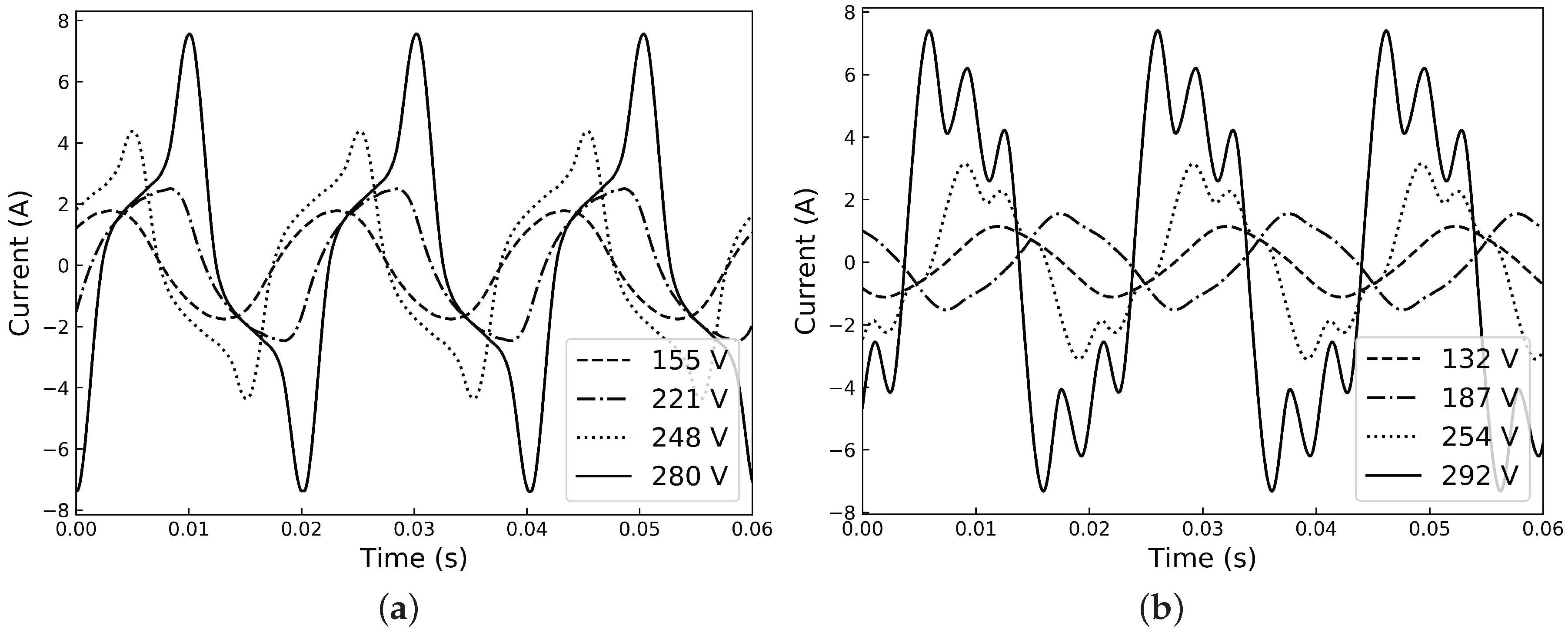
3. Result and Discussion

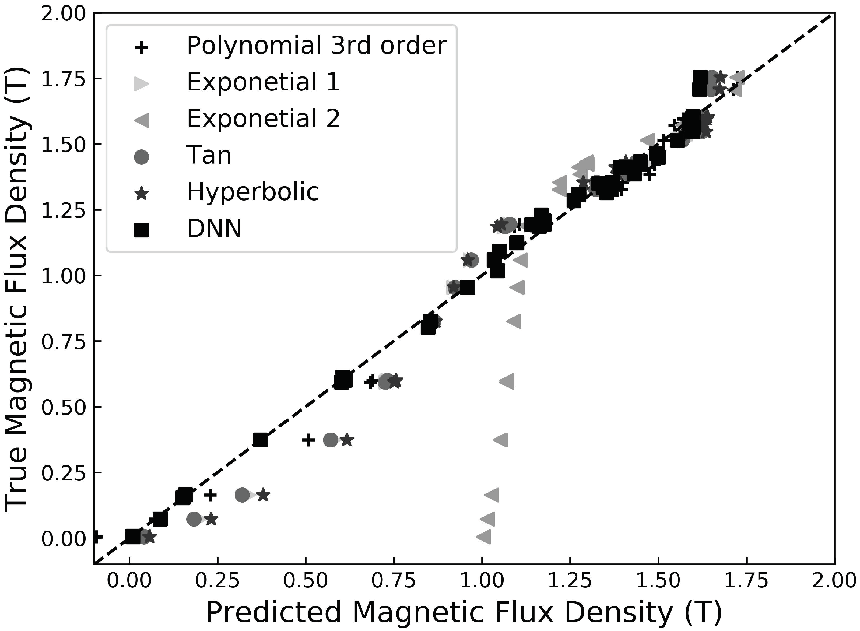
3.1. Magnetization Modeling

The typical currents measured from the three-phase transformer are presented in Figure 3a,b, where Figure 3a presents the measured currents under several voltages from B-phase excitation, and Figure 3b presents currents from three-phase excitation.

The current distortions of both excitation types were significant, and larger excitation voltages cause larger asymmetric characteristic with sharper peaks. In addition, up to three peaks were observed in a half cycle under high voltage three-phase excitation. It is known that this distortion is caused by the overall nonlinear relationship between the magnetic field strength and magnetic flux density of the transformer core. Based on the on-line measured currents and voltages from the operating transformer and Equations (1) and (2), the corresponding hysteresis loops and magnetization curve were calculated and are shown in Figure 4.

From Figure 4, the curves with darker color were the hysteresis loops under larger voltage excitation. The smaller loops caused by the lower excitation voltages are contained within the larger loops with high excitation voltages. The magnetization curve can be drawn by connecting their vertex points, as presented by the black line in Figure 4. A three-layer DNN is used for modeling this magnetization curve; the predictions are shown in Figure 5 along with the result from other methods on the testing set.

Table 1. Performance of different magnetization curve model.

Model	RMSE	Correlation Coefficient
Neural Network	0.0013	99.95%
Polynomial	0.0079	99.47%
Hyperbolic	0.0236	98.09%
Exponential 1	0.0211	98.84%
Exponential 2	0.1207	83.12%
Transcendental	0.0198	98.89%

shows the RMSE and correlation coefficients of different models in a testing set.

In Figure 5, the black squares represent the DNN predictions in x-axis and real values in y-axis. Other markers represent results from other models, as shown in the legend. The dashed black line represents the condition with predicted values equal to the real ones, called the ideal performance curve. The DNN predictions lie on the ideal performance curve with little error while the predictions from other models present significant bias, especially in the low range of the magnetic flux density. The second exponential model from (10) has the worst performance (black triangles) with large error when magnetic flux density smaller than 1.2 T; the polynomial from 7 (black stars) has the closest performance to the DNN. As shown in Table 1, the RMSE of DNN is at least $\frac{1}{6}$ of the other models and the correlation coefficient almost equals to 1. The second exponential model has the largest RMSE value and lowest correlation coefficients, and performance from the polynomial model are closest to the ones from DNN. The above result shows that the DNN is better than the other traditional models in both the RMSE and correlation coefficient. In addition, compared to previous research in [22], where the best model achieved a 99.92% correlation coefficient, the proposed DNN model in this paper also achieves the best performance. Finally, the magnetization curve from DNN is given in Figure 6 and the saturation magnetic flux density is around 1.7 T.

The SVR is used for calculating $H_c$ and $H_{amp}$ under different excitation voltages. Different kernels like RBF, logistic and polynomial regression were tried for comparison and the RBF with penalty parameter C equals 1000 and $\gamma$ equals to 0.0001 achieved the best performance with 96% and 97% correlation coefficients for $H_c$ and $H_{amp}$, respectively.

Figure 7a,b show the prediction results within the range of 0–300 V. With higher excitation voltage, the $H_{amp}$ increases more significantly as the flux density is already saturated. Whilst the $H_c$ starts to saturate when voltage increases. The significant increase of $H_{amp}$ and small increase of $H_c$ in large voltage excitation indicate its small hysteresis loss of the silicon steel. Due to their nonlinear behavior, the Wlodarski model can achieve much higher accuracy in capturing these two points of the hysteresis loops compare to the linear scaling, as shown by the dashed line in Figure 7. The RMSE of $H_{amp}$ and $H_c$ from linear scaling are 27.0 and 7.94 A/m and the proposed model are approximate $\frac{1}{8}$ of them, as 3.83 and 0.822 A/m, respectively. Finally, accurate $H_{amp}$ and $H_c$ under various excitation are obtained.

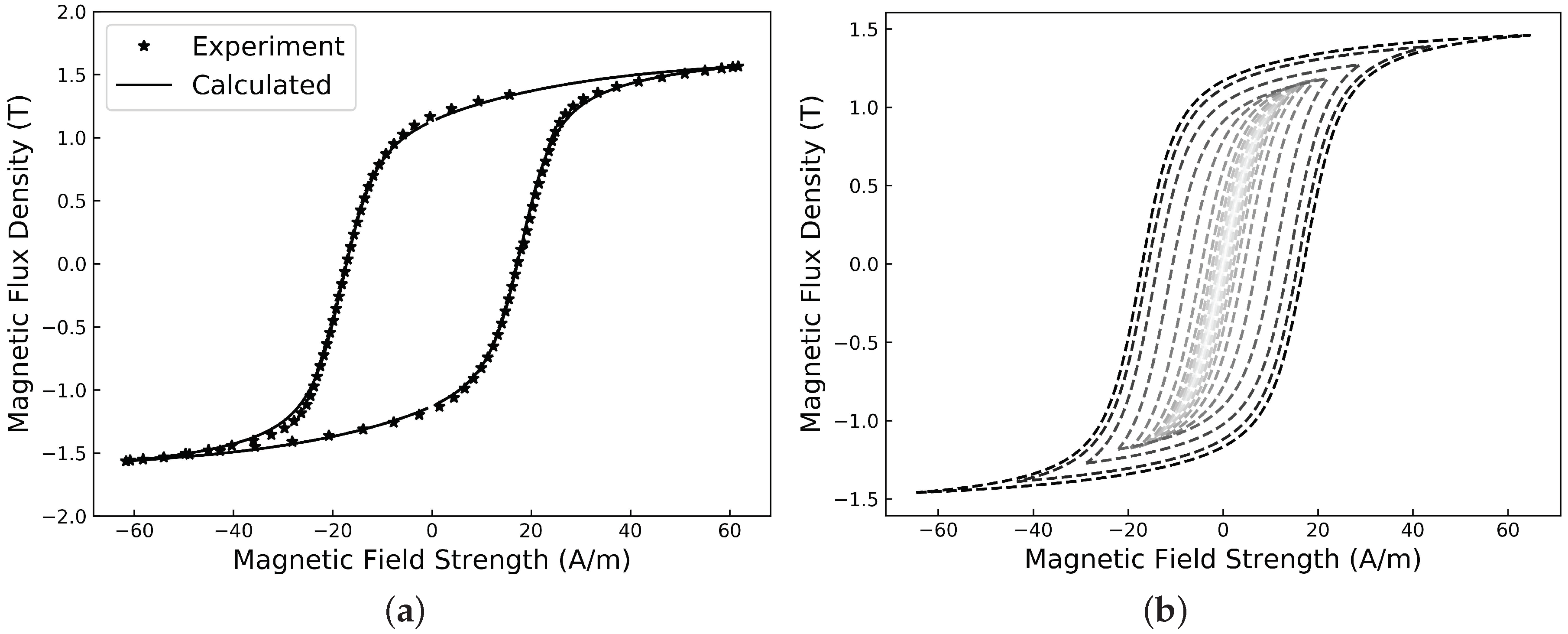
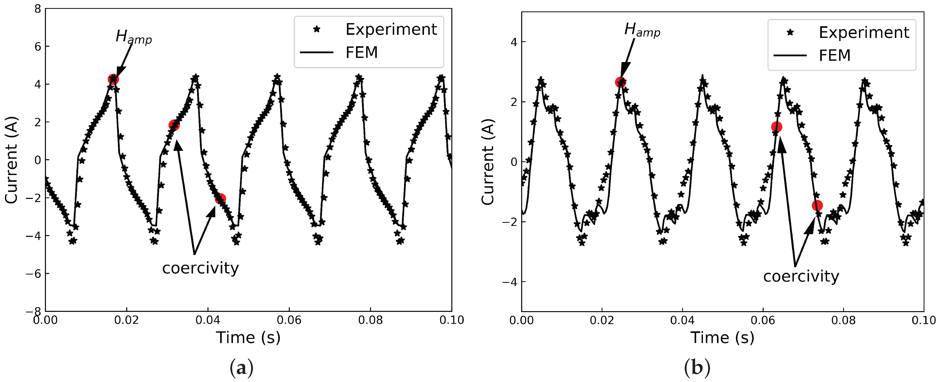
3.2. Hysteresis Loop Simulation

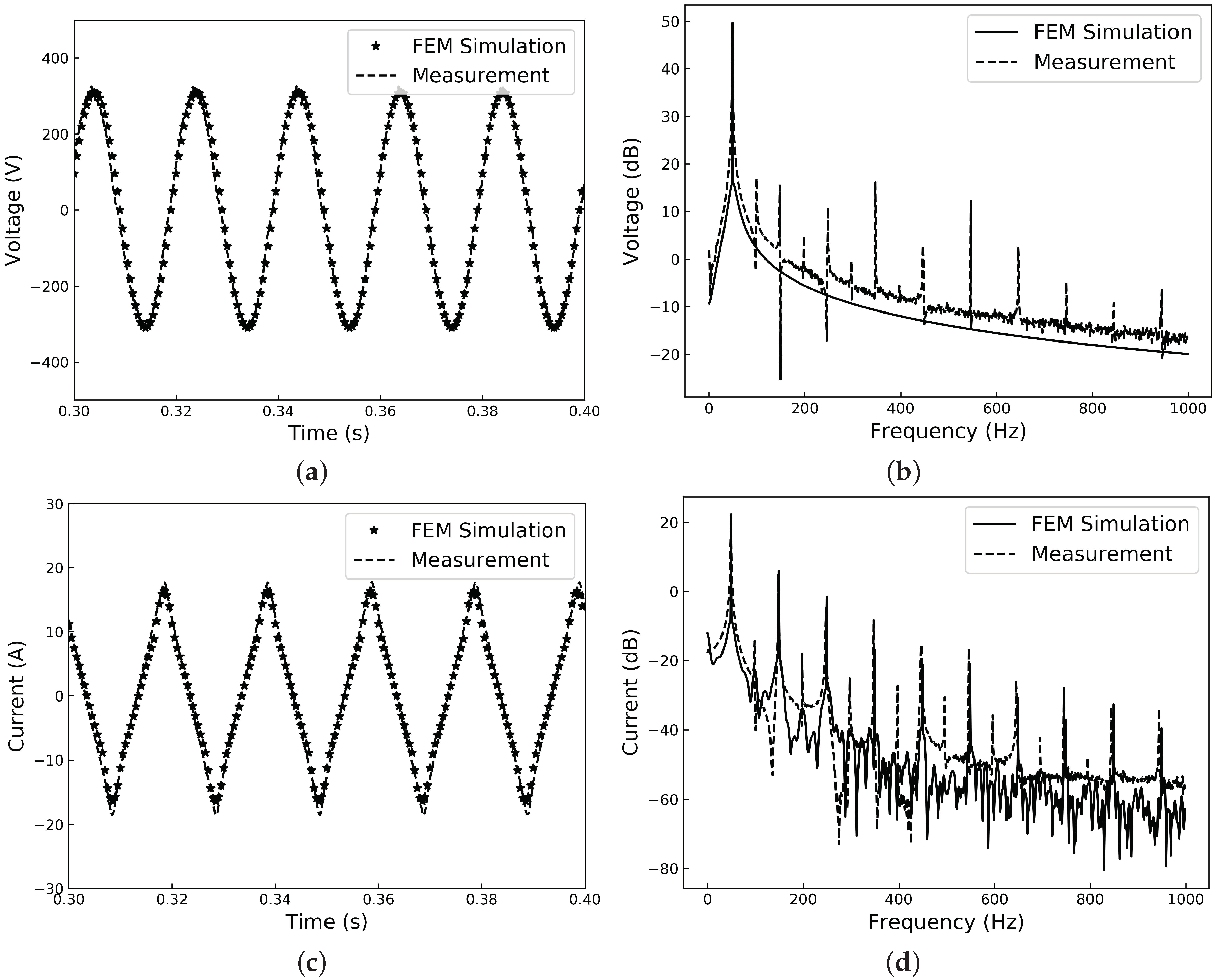
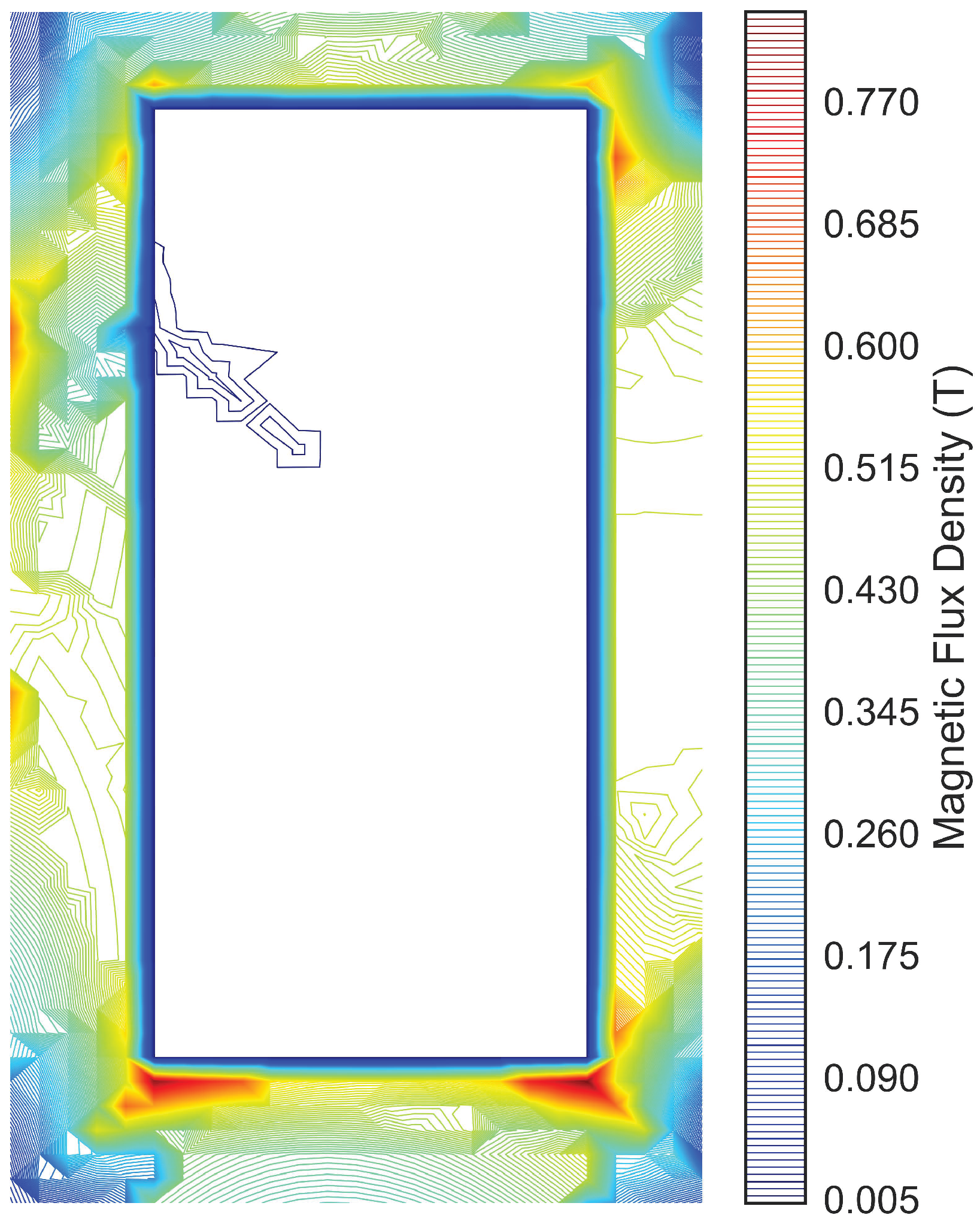
By obtaining $H_c$ and $H_{amp}$ under different excitation voltages from the SVR model, the Wlodarski model, Equations (16)–(19), is used to calculate the overall hysteresis loop under any voltage excitation.

Figure 8a illustrates the calculated hysteresis loops from the Wlodarski model (solid black curve) compared with loops from the on-line experimental data (black stars). The two components of saturation magnetization $M_a$ and $M_b$ are 1.15 and 0.25 MA/m, respectively. The rates approach saturation a and b are 21.1 and 2.89 A/m, respectively. The family of hysteresis loops under various voltage excitation is approximated from the Wlodarski model using the same optimal parameters and shown in Figure 8b, where darker curves represent the hysteresis loops under larger voltage excitation. By using these hysteresis loops, the transformer magnetic flux and excitation current are able to be calculated and $H_c$ and $H_{amp}$ can be captured accurately. Since these simulated hysteresis loops describe the overall hysteresis characteristic of the transformer, they can be applied to calculate, not only the magnetization current and magnetic field of the transformer, but also the corresponding iron loss by combining Bertotti’s model or other methods [23,24].

3.3. Applications

FEM is used to simulate the excitation current by accounting for the hysteresis loops in the material properties (permeability setting). The results are compared with two experimental measurements. Figure 9a,b show the comparison between the FEM simulation result (black line) and the on-line data (black dot) under 270 V of both B-phase and three-phase excitation. Hysteresis loops in Figure 8b were applied in the FEM. The results show that the hysteresis characteristics appear in the current undert both excitation settings. The FEM simulated current matched the on-line current under both B-phase excitation, with 98.6% correlation coefficient and three-phase excitation with 96.5%. In addition, the simulated current shows three peaks in a half cycle under three-phase excitation like the on-line data. As mentioned above, since the hysteresis loops are calculated from on-line current and voltage under B-phase excitation, the high correlation coefficient between the on-line and FEM simulated current under three-phase excitation reflect the accuracy of these calculated hysteresis loops, which are calculated by combining the Wlodarski model, SVR and on-line experimental data. The critical points for magnetic field simulation, the $H_c$ and $H_{amp}$, are predicted accurately as highlighted by the red dots in Figure 9.

Similar result can be drawn from another simulation and experiment on a single-phase transformer. The FEM calculated current and voltage under 240 V voltage are shown in Figure 10. The FEM simulation voltage and current are closed to the measured result with 96% and 97% correlation coefficients, respectively. From Figure 10b, the measured amplitude of the fundamental frequency is at least 30 dB larger than the other frequencies, which cause the harmonic negligible. On the other hand, from Figure 10d, the difference between the current fundamental frequency and its harmonic is less than 20 dB and, hence, the harmonics are shown to be important. In this case, the current from FEM also performs a good agreement in its harmonic. From this result, the feasibility of the proposed method is indicated. Finally, the simulated magnetic flux density of the single phase transformer is presented in Figure 11.

Figure 11 shows a reasonable result of magnetic flux density distribution on the middle slice of the single phase transformer from FEM simulation under 240 V. According to the simulation, four inner corners have the strongest flux density around 0.8 T and the outer corners display much smaller values. This phenomenon can be explained by the difference of the length of the magnetic paths. When the structure material is the same, the shorter length of the magnetic path, the smaller magnetic reluctance it will have. Therefore, the flux density of the inner corner is much stronger than the outer one because the magnetic flux has the tendency to follow the path with low magnetic reluctance. The flux density at the middle range of the limb is fairly constant with small variation. In addition, since the existence of the 2-mm air gap on the left limb, some disturbance is observed and the leakage flux at the gap region is relatively strong.

Based on the above experimental and FEM results, the proposed method for calculating the overall B–H relationship including the magnetization curve and hysteresis loops under AC excitation by using machine learning algorithms and on-line data seems useful.

4. Conclusions

Based on limited on-line currents and voltages of a three-phase transformer under B-phase excitation, the overall magnetization curve and hysteresis loops under alternating current excitation were calculated using a deep neural network, support vector regressor and Wlodarski model. The magnetization curve was modeled by a deep neural network with 99.95% correlation coefficient and the coercivity and amplitude of magnetic field strength were modeled by a support vector regressor with 96% and 97% correlation coefficients. By applying these characteristics to the Wlodarski model, the hysteresis loops under different alternating voltage excitations of the transformer can be calculated with high accuracy, especially for capturing the coercivity and the amplitude of magnetic field strength, which is important for calculating the critical features of the magnetic field. The calculated hysteresis loops were applied into a finite element method for current and magnetic field simulation; experiments on the three-phase transformer under three-phase excitation and on the single phase transformer were conducted for comparison. The results showed the usefulness of this method with high correlation coefficients between the experimental data and the finite element model calculations. The simulated magnetic field distribution also presents a reasonable result. Using this method, the actual magnetic field variation inside the transformer core can be modeled on-line. In turn, this information could be used for force density calculation in predicting the vibration of power transformers.

References

1. Schulz, M.; Ringlee, R. Some characteristics of audible noise of power transformers and their relationship to audibility criteria and noise ordinances. Trans. Am. Inst. Electr. Eng. 1960, 79, 316–322. [Google Scholar] [CrossRef]
2. Salvini, A.; Fulginei, F.R. Genetic algorithms and neural networks generalizing the Jiles–Atherton model of static hysteresis for dynamic loops. IEEE Trans. Magn. 2002, 38, 873–876. [Google Scholar] [CrossRef]
3. Jiles, D.; Ramesh, A.; Shi, Y.; Fang, X. Application of the anisotropic extension of the theory of hysteresis to the magnetization curves of crystalline and textured magnetic materials. IEEE Trans. Magn. 1997, 33, 3961–3963. [Google Scholar] [CrossRef] [Green Version]
4. Liorzou, F.; Phelps, B.; Atherton, D. Macroscopic models of magnetization. IEEE Trans. Magn. 2000, 36, 418–428. [Google Scholar] [CrossRef]
5. De Leon, F.; Semlyen, A. A simple representation of dynamic hysteresis losses in power transformers. IEEE Trans. Power Del. 1995, 10, 315–321. [Google Scholar] [CrossRef]
6. Li, C.; Tan, Y. Modelling Preisach-type hysteresis nonlinearity using neural network. Int. J. Model. Simul. 2007, 27, 233–241. [Google Scholar] [CrossRef]
7. Lin, C.E.; Cheng, C.L.; Huang, C.L. Hysteresis characteristic analysis of transformer under different excitations using real time measurement. IEEE Trans. Power Deliv. 1991, 6, 873–879. [Google Scholar] [CrossRef]
8. Benšić, T.; Biondić, I.; Marić, P. Single-phase autotransformer modelling and model parameter identification. Electr. Eng. 2018, 100, 625–632. [Google Scholar] [CrossRef]
9. Freitag, C.I. Magnetic Properties of Electrical Steel, Power Transformer Core Losses and Core Design Concepts. Ph.D. Thesis, Karlsruhe Institute of Technology, Karlsruhe, Germany, 2017. [Google Scholar]
10. Mayergoyz, I.; Friedman, G. Generalized Preisach model of hysteresis. IEEE Trans. Magn. 1988, 24, 212–217. [Google Scholar] [CrossRef]
11. Sadowski, N.; Batistela, N.; Bastos, J.; Lajoie-Mazenc, M. An inverse Jiles–Atherton model to take into account hysteresis in time-stepping finite-element calculations. IEEE Trans. Magn. 2002, 38, 797–800. [Google Scholar] [CrossRef]
12. Wlodarski, Z. Modeling hysteresis by analytical reversal curves. Phys. B Condens. Matter 2007, 398, 159–163. [Google Scholar] [CrossRef]
13. Wlodarski, Z. Extraction of hysteresis loops from main magnetization curves. J. Magn. Magn. Mater. 2007, 308, 15–19. [Google Scholar] [CrossRef]
14. Lin, G.; Song, Q.; Wang, L.; Zhang, D.; Pan, F. A hybrid algorithm based on fish swarm and simulated annealing for parameters identification of modified JA model. In Proceedings of the IEEE International Conference on Electronic Measurement & Instruments (ICEMI), Yangzhou, China, 20–22 October 2017; pp. 483–488. [Google Scholar]
15. Saghafifar, M.; Kundu, A.; Nafalski, A. Dynamic magnetic hysteresis modelling using Elman recurrent neural network. Int. J. Appl. Electromagn. Mech. 2001, 13, 209–214. [Google Scholar]
16. Deželak, K.; Pihler, J. Artificial Neural Network as Part of a Saturation-Level Detector within the Transformer’s Magnetic Core. IEEE Trans. Magn. 2016, 52, 1–4. [Google Scholar] [CrossRef]
17. Dommel, H.W. Electromagnetic Transients Program: Reference Manual: (EMTP Theory Book); Bonneville Power Administration: Portland, OR, USA, 1986.
18. Casoria, S.; Sybille, G.; Brunelle, P. Hysteresis modeling in the MATLAB/power system blockset. Math. Comput. Simul. 2003, 63, 237–248. [Google Scholar] [CrossRef]
19. Hinton, G.; Deng, L.; Yu, D.; Dahl, G.E.; Mohamed, A.r.; Jaitly, N.; Senior, A.; Vanhoucke, V.; Nguyen, P.; Sainath, T.N.; Kingsbury, B. Deep neural networks for acoustic modeling in speech recognition: The shared views of four research groups. IEEE Signal Process. Mag. 2012, 29, 82–97. [Google Scholar] [CrossRef]
20. Liu, L.; Wang, S.; Zhao, Z. Radar Waveform Recognition Based on Time-Frequency Analysis and Artificial Bee Colony-Support Vector Machine. Electronics 2018, 7, 59. [Google Scholar] [CrossRef]
21. Sandeep, V.; Murthy, S.; Singh, B. A comparative study on approaches to curve fitting of magnetization characteristics for induction generators. In Proceedings of the IEEE International Conference on Power Electronics, Drives and Energy Systems (PEDES), Bengaluru, India, 16–19 December 2012; pp. 1–6. [Google Scholar]
22. Tang, Q.; Wang, Z.; Anderson, P.I.; Jarman, P.; Moses, A.J. Approximation and prediction of AC magnetization curves for power transformer core analysis. IEEE Trans. Magn. 2015, 51, 1–8. [Google Scholar] [CrossRef]
23. Bertotti, G.; Fiorillo, F.; Soardo, G. The prediction of power losses in soft magnetic materials. J. Phys. Colloq. 1988, 49, C8-1915–C8-1919. [Google Scholar] [CrossRef]
24. Štumberger, B.; Goričan, V.; Štumberger, G.; Hamler, A.; Trlep, M.; Jesenik, M. Accuracy of iron loss calculation in electrical machines by using different iron loss models. J. Magn. Magn. Mater. 2003, 254, 269–271. [Google Scholar] [CrossRef]
Figure 1. The three-layer DNN structure with six and three nodes in two hidden layers, respectively.
Electronics 07 00390 g001
Figure 2. The configurations of (a) the three-phase and (b) the single-phase transformer cores.
Electronics 07 00390 g002
Figure 3. The measured current of the three-phase transformer under different excitation voltages with (a) B-phase excitation and (b) three-phase excitation.
Electronics 07 00390 g003
Figure 4. The hysteresis loops calculated from on-line experimental data under several excitation voltages.
Electronics 07 00390 g004
Figure 5. The performance of magnetization curves fitting with different models including DNN, 3rd degree polynomial, hyperbolic, two exponential functions, and transcendental functions.
Electronics 07 00390 g005
Figure 6. Magnetization curve calculated from DNN based on on-line experimental data.
Electronics 07 00390 g006
Figure 7. The SVR prediction of (a) H c and (b) H a m p under different excitation voltages.
Electronics 07 00390 g007
Figure 8. (a) The fitting of the Wlodarski model compared with the experiment data; (b) The calculated hysteresis loops from Wlodarski model with darker curve represents the hysteresis loop under larger voltage excitation.
Electronics 07 00390 g008
Figure 9. The comparison between the FEM and experiment results of 270 V excitation under (a) B-phase and (b) three-phase excitation.
Electronics 07 00390 g009
Figure 10. Comparison between the FEM and experimental result in (a) voltage; (b) voltage spectrum; (c) current; and (d) current spectrum on the single phase transformer.
Electronics 07 00390 g010
Figure 11. The simulated magnetic contour field of the single phase transformer.
Electronics 07 00390 g011