Comparison of Different Repetitive Control Architectures: Synthesis and Comparison. Application to VSI Converters

Abstract

Repetitive control is one of the most used control approaches to deal with periodic references/disturbances. It owes its properties to the inclusion of an internal model in the controller that corresponds to a periodic signal generator. However, there exist many different ways to include this internal model. This work presents a description of the different schemes by means of which repetitive control can be implemented. A complete analytic analysis and comparison is performed together with controller synthesis guidance. The voltage source inverter controller experimental results are included to illustrative conceptual developments.

1. Introduction

Repetitive Control (RC) [1,2,3,4,5] is founded on the well-known Internal Model Principle (IMP) [6,7], which establishes that to track/reject a reference/disturbance with null steady-state error the reference/disturbance generator must be included in the control loop. RC focuses on the case of periodic references/disturbances [8] and has been used in many different applications like power electronics [8] or mechatronic systems [9], among others.

Periodical signals generators are usually very high order marginally-stable dynamic systems. Although conventional stabilizing techniques could be used, the achieved controllers would be very high order. This implies huge computational resources and fragility problems, which make the implementation difficult. In order to overcome these problems, specific architectures and anti-windup techniques [10,11,12] have been developed to profit from RC’s nice steady-state properties while using low computational resources and reducing fragility problems.

These specific architectures have used the z-transform formalism [13,14] and the state-space [15,16,17] one. Although the state-space formalism offers a more generic and elegant formalism, this work will focus on summarizing the z-transform-based architectures, which offer a more compact and close to real practice framework.

With the appearance and improvement of the new sources of renewable energy, the design of new typologies and control systems for Voltage Source Inverters (VSI) [18,19] has taken on great relevance in recent times. RC is one of the control techniques that has been extensively used to control VSI. In this work, the described RC architectures will be applied to the VSI control, and the complete design and experimental results will be included in the paper.

The current work is organized as follows: Section 2 contains an introduction to the internal models and architectures used in repetitive control systems; in Section 3, the design of RC for a VSI will be developed and experimentally validated; finally, in Section 4, some final summarizing comments and discussions are included.

2. Repetitive Control Basics and Architectures

This section describes repetitive control’s most relevant concepts and architectures. Section 2.1 describes the generator for the most popular periodical signals; Section 2.2 describes the series architecture, which is the simplest way to implement a repetitive controller; in Section 2.3, the plug-in structure, which was the first proposed architecture, will be described; in Section 2.4; a disturbance observer approach will be discussed; in Section 2.5, the Youla parametrization will be presented; and finally, Section 2.6 will describe an $H_{\infty }$ optimization approach.

2.1. Periodical Signal Generator

The periodical signal generator, i.e., the internal model, is the most relevant element in an RC system, and it is composed of a dynamic system that can generate the desired periodic signal. Figure 1 contains a generic block scheme, composed of a positive feedback system, which allows constructing the most relevant periodical signal generators used in RC.

$$I\left(z\right)=\frac{U_r\left(z\right)}{E\left(z\right)}=\frac{\sigma H\left(z\right)W\left(z\right)}{1-\sigma H\left(z\right)W\left(z\right)},$$

(1)

where $\sigma =\left\{-1,1\right\}$, $W\left(z\right)$ is the time delay function, and $H\left(z\right)$ is a FIR low-pass filter introduced to improve the system robustness. As an example, for $\sigma =1$, $W\left(z\right)=z^{-N}$ and $H\left(z\right)=1$, an N-periodic generator, $I\left(z\right)=\frac{1}{z^N-1}$, is obtained. and for $\sigma =-1$, $W\left(z\right)=z^{-\frac{N}{2}}$, and $H\left(z\right)=1$, the odd-harmonic generator [20] is obtained $I\left(z\right)=\frac{-1}{z^{\frac{N}{2}}+1}$. By selecting $\sigma$ and $W\left(z\right)$ appropriately, different harmonic patterns can be selected.

Table 1. Periodical signal generators used in Repetitive Control (RC). HORC, High Order RC.

Harmonics	RC	HORC
Full	$\begin{array}{c}I\left(z\right)=\frac{H\left(z\right)}{z^N-H\left(z\right)}\\ W\left(z\right)=z^{-N},\sigma =1\end{array}$	$\begin{array}{c}I\left(z\right)=\frac{W\left(z\right)H\left(z\right)}{1-W\left(z\right)H\left(z\right)}\\ W\left(z\right)=1-{\left(1-z^{-N}\right)}^M,\sigma =1\end{array}$
Odd	$\begin{array}{c}I\left(z\right)=\frac{-H\left(z\right)}{z^{\frac{N}{2}}+H\left(z\right)}\\ W\left(z\right)=z^{-\frac{N}{2}},\sigma =-1\end{array}$	$\begin{array}{c}I\left(z\right)=\frac{-W\left(z\right)H\left(z\right)}{1+W\left(z\right)H\left(z\right)}\\ W\left(z\right)=-1+{\left(1+z^{-\frac{N}{2}}\right)}^M,\sigma =-1\end{array}$
$6l\pm 1$ [23]	$\begin{array}{c}I\left(z\right)=\frac{W\left(z\right)H\left(z\right)}{1+W\left(z\right)H\left(z\right)}\\ W\left(z\right)=z^{-\frac{N}{3}}-z^{-\frac{N}{6}},\sigma =-1\end{array}$	-

contains different values for $W\left(z\right)$ and $\sigma$ and its related signal generators. The table also contains High Order Repetitive Control (HORC) generators, which can be used to improve the robustness against signal frequency variations [21,22].

When $H\left(z\right)=1$, the achieved generators, $I\left(z\right)$, introduce infinite gain at the selected harmonics (full, odd, etc.). This high gain at high frequencies might be a problem in the presence of uncertainty. To reduce this gain, a FIR low-pass filter, $H\left(z\right)$, is usually used. A null-phase low-pass filter is commonly used [20,24]. The null-phase characteristic avoids the frequency shift of the internal model poles.

When $I\left(z\right)=\frac{N_I\left(z\right)}{D_I\left(z\right)}$ is included in a closed-loop control system, the sensitivity function, $S\left(z\right)=\frac{E\left(z\right)}{R\left(z\right)}$, will include the polynomial $D_I\left(z\right)$ in its numerator. In this way, poles of $I\left(z\right)$ become zeros of $S\left(z\right)$, i.e., the frequencies corresponding to the poles of $I\left(z\right)$ will not appear in the error signal in the steady-state.

2.2. Series Approach

In general, an open-loop system composed by a series connection of the generator, $I\left(z\right)$, and the plant, $G\left(z\right)$, would produce an unstable closed-loop system. Due to this, it is necessary to use a stabilizing controller, $G_c\left(z\right)$. The most straightforward manner to do this is putting $G_c\left(z\right)$ in series connection jointly with the generator, $I\left(z\right)$, and the plant, $G\left(z\right)$, as shown in Figure 2. Consequently, the controller becomes:

$$C\left(z\right)=\frac{U\left(z\right)}{E\left(z\right)}=I\left(z\right)G_c\left(z\right).$$

(2)

With this controller and the structure shown Figure 2, the complementary sensitivity and sensitivity functions are:

$$\begin{array}{ccc}\hfill T\left(z\right)& =& \frac{Y\left(z\right)}{R\left(z\right)}=\frac{I\left(z\right)G_c\left(z\right)G\left(z\right)}{1+I\left(z\right)G_c\left(z\right)G\left(z\right)},\hfill \end{array}$$

(3)

$$\begin{array}{ccc}\hfill S\left(z\right)& =& \frac{E\left(z\right)}{R\left(z\right)}=\frac{1}{1+I\left(z\right)G_c\left(z\right)G\left(z\right)}.\hfill \end{array}$$

(4)

Obtaining the appropriate $G_c\left(z\right)$ might be a challenging problem in general. For minimum-phase plants, $G_c\left(z\right)$, a methodology that offers nice results is:

$$G_c\left(z\right)=\frac{k_r}{G\left(z\right)}.$$

(5)

Under this hypothesis, the closed-loop transfer functions become:

$$\begin{array}{ccc}\hfill T\left(z\right)& =& \frac{k_r\sigma W\left(z\right)H\left(z\right)}{1+(k_r-1)\sigma W\left(z\right)H\left(z\right)},\hfill \end{array}$$

(6)

$$\begin{array}{ccc}\hfill S\left(z\right)& =& \frac{1-\sigma W\left(z\right)H\left(z\right)}{1+(k_r-1)\sigma W\left(z\right)H\left(z\right)}.\hfill \end{array}$$

(7)

As expected, $S\left(z\right)$ has in the numerator the denominator of $I\left(z\right)$.

In the case of non-minimum-phase plants, this approach cannot be directly applied; instead, the phase cancellation methodology can be used to select $G_c\left(z\right)$ [25,26].

In the case of plants described by a nominal model plus multiplicative uncertainty: $G\left(z\right)=G_n(1+W_u^m\left(z\right)\Delta \left(z\right))$ [27], it is possible to determine a robust stability condition, which takes the following form:

$${∥W_u^m\left(z\right)\frac{k_r\sigma W\left(z\right)H\left(z\right)}{1+(k_r-1)\sigma W\left(z\right)H\left(z\right)}∥}_{\infty }<1.$$

(8)

As $\sigma$ and $W\left(z\right)$ are selected by fixing the desired harmonic pattern, $H\left(z\right)$ and $k_r$ can be designed so that the robust stability condition is guaranteed. This RC architecture is by far the simplest RC architecture described in the literature.

2.3. Plug-in Approach

The most popular approach in RC is the plug-in architecture (Figure 3). This architecture introduces the generator, $I\left(z\right)$, as a complement to a previously-existing controller $G_c\left(z\right)$. The goal of this internal controller is to guarantee closed-loop stability and robustness to the control system without the generator’s influence. Later, the internal model, $I\left(z\right)$, and the stabilizing controller, $G_x\left(z\right)$, are plugged into the previous closed-loop system, as shown in Figure 3.

In this case, the closed-loop transfer function can be constructed in terms of the closed-loop transfer function without the internal model:

$$\begin{array}{ccc}\hfill S_o\left(z\right)& =& \frac{1}{1+G_c\left(z\right)G\left(z\right)}\hfill \end{array}$$

(9)

$$\begin{array}{ccc}\hfill T_o\left(z\right)& =& \frac{G_c\left(z\right)G\left(z\right)}{1+G_c\left(z\right)G\left(z\right)}\hfill \end{array}$$

(10)

and a modifying term:

$$\begin{array}{ccc}\hfill S_{Mod}\left(z\right)& =& \frac{1-\sigma W\left(z\right)H\left(z\right)}{1-\sigma W\left(z\right)H\left(z\right)\left(1-G_x\left(z\right)T_o\left(z\right)\right)}.\hfill \end{array}$$

(11)

Therefore, the closed-loop transfer functions are:

$$\begin{array}{ccc}\hfill S\left(z\right)& =& \frac{E\left(z\right)}{R\left(z\right)}=S_o\left(z\right)S_{Mod}\left(z\right)\hfill \end{array}$$

(12)

$$\begin{array}{ccc}\hfill T\left(z\right)& =& \frac{Y\left(z\right)}{R\left(z\right)}=\frac{\left(1-\sigma W\left(z\right)H\left(z\right)\left(1-G_x\left(z\right)\right)\right)T_o\left(z\right)}{1-\sigma W\left(z\right)H\left(z\right)\left(1-G_x\left(z\right)T_o\left(z\right)\right)}.\hfill \end{array}$$

(13)

For minimum-phase plants (for non-minimum phase plants, a phase cancellation approach is usually used), the most popular form of the stabilizing controller is:

$$G_x\left(z\right)=\frac{k_r}{T_o\left(z\right)}.$$

(14)

With this selection, the closed-loop function becomes:

$$\begin{array}{ccc}\hfill S\left(z\right)& =& \frac{E\left(z\right)}{R\left(z\right)}=S_o\left(z\right)\frac{1-\sigma W\left(z\right)H\left(z\right)}{1+\left(k_r-1\right)\sigma W\left(z\right)H\left(z\right)}\hfill \end{array}$$

(15)

$$\begin{array}{ccc}\hfill T\left(z\right)& =& \frac{Y\left(z\right)}{R\left(z\right)}=\frac{\left(T_o\left(z\right)-\sigma W\left(z\right)H\left(z\right)\left(T_o\left(z\right)-k_r\right)\right)}{1+\left(k_r-1\right)\sigma W\left(z\right)H\left(z\right)}.\hfill \end{array}$$

(16)

The complete control system is:

$$\begin{array}{ccc}\hfill C\left(z\right)=\frac{U\left(z\right)}{E\left(z\right)}& =& \left(1+I\left(z\right)·G_x\left(z\right)\right)G_c\left(z\right)\hfill \end{array}$$

(17)

$$\begin{array}{cc}=& \left(1+\frac{\sigma H\left(z\right)W\left(z\right)}{1-\sigma H\left(z\right)W\left(z\right)}\frac{k_r\left(1+G_c\left(z\right)G\left(z\right)\right)}{G_c\left(z\right)G\left(z\right)}\right)G_c\left(z\right).\hfill \end{array}$$

(18)

The following two conditions guarantee closed-loop stability [8]:

• $T_o\left(z\right)$ must be stable ($G_c\left(z\right)$ can be designed to fulfill it)
• $\parallel W\left(z\right)H\left(z\right)\left(1-k_r\right){\parallel }_{\infty }<1$ ($k_r$ can be selected appropriately)

Even thought these conditions are only sufficient, it has been claimed that they are close to the necessary ones in practice [28].

It is important to emphasize that in (14), the inversion of $T_o\left(z\right)$ is required, while in (5), the inversion of $G\left(z\right)$ is required; as $T_o\left(z\right)$ is a closed-loop system, its uncertainty should be less than that of $G\left(z\right)$. Additionally, it is important to visualize that the sensitivity function in the series approach and the plug-in one is the same, except the $S_o\left(z\right)$ term, which can be appropriately shaped using $G_c\left(z\right)$.

In the case of plants subject to multiplicative uncertainty, the robust stability condition becomes:

$${∥W_u^m\left(z\right)\frac{\left(T_o\left(z\right)-\sigma W\left(z\right)H\left(z\right)\left(T_o\left(z\right)-k_r\right)\right)}{1+\left(k_r-1\right)\sigma W\left(z\right)H\left(z\right)}∥}_{\infty }<1.$$

(19)

This condition is quite similar to the one obtained in the series architecture (Section 2.2), but it contains $T_o\left(z\right)$. This term can be shaped using $G_c\left(z\right)$, so it is simpler to fulfill this constraint than the one obtained in the series approach.

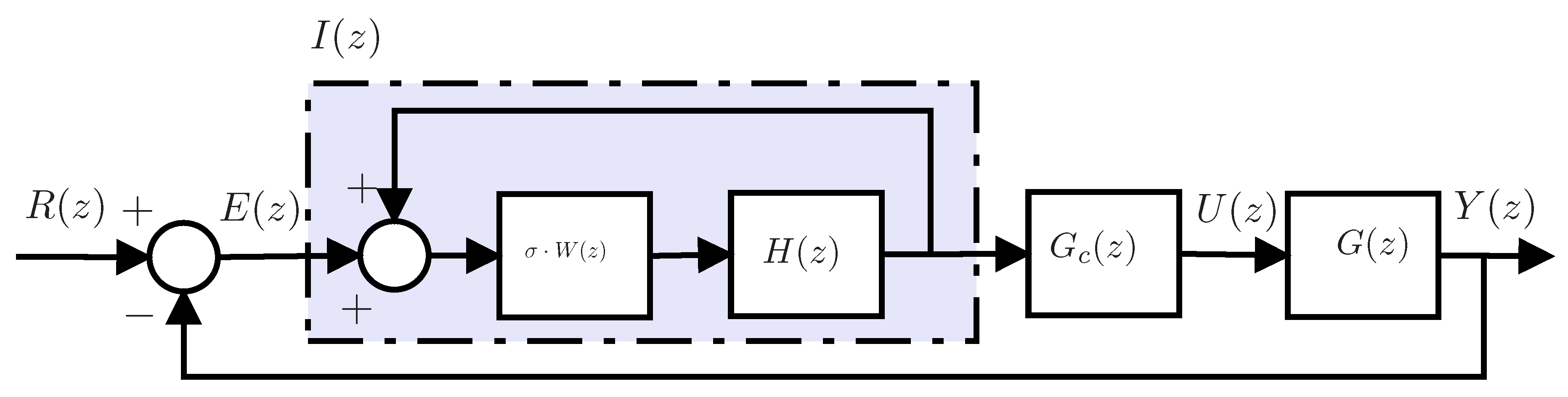
2.4. Disturbance Rejection Approach

In recent years, a great effort has been made to propose new disturbance rejection mechanisms [29]. As one of RC’s nice properties is to reject periodic disturbances, it is possible to think of RC as a disturbance observer; in this framework an RC architecture has been proposed [13]. Its characteristics are analyzed in this section.

Figure 4 shows a disturbance rejection diagram for an m-relative degree minimum phase plant, $G\left(z\right)$. The control system is composed by a stabilizing controller, $G_c\left(z\right)$, plus a disturbance observer composed by the plant model and a filter $Q\left(z\right)$. The goal of the disturbance observer is to estimate $D\left(z\right)$ so it can be rejected. In this scheme, $Q\left(z\right)$ is usually a low-pass filter in charge of handling plant uncertainties.

The sensitivity function for the closed-loop system in Figure 4 is given by:

$$S\left(z\right)=\frac{E\left(z\right)}{R\left(z\right)}=\frac{1-z^{-m}Q\left(z\right)}{1+G\left(z\right)G_c\left(z\right)}.$$

(20)

To transform this into the sensitivity function obtained with an RC, it is necessary to select $Q\left(z\right)$ so that the generator’s, $I\left(z\right)$, denominator appears in the numerator of $S\left(z\right)$. Therefore, $Q\left(z\right)$ should be obtained from the following equation:

$$\frac{1-z^{-m}Q\left(z\right)}{1+G\left(z\right)G_c\left(z\right)}=S_o\left(z\right)\left(1-\sigma W\left(z\right)H\left(z\right)\right)\frac{N_s\left(z\right)}{D_s\left(z\right)}$$

(21)

where $N_s\left(z\right)$ and $D_s\left(z\right)$ are polynomials that must be fixed (this selection requires $S_o\left(z\right)$ to be stable, which can be achieved using $G_c\left(z\right)$). Finally,

$$Q\left(z\right)=z^m\frac{\left(1-\sigma W\left(z\right)H\left(z\right)\right)N_s\left(z\right)-D_s\left(z\right)}{D_s\left(z\right)}.$$

(22)

Although other possibilities exist, a simple option is choosing $N_s\left(z\right)=1$ and $D_s\left(z\right)=1-\alpha ·\sigma ·W\left(z\right)H\left(z\right)$ with $\left|\alpha \right|<1$, which generates:

$$Q\left(z\right)=z^m\frac{-(1+\alpha )·\sigma W\left(z\right)H\left(z\right)}{1-\alpha ·\sigma ·W\left(z\right)H\left(z\right)}.$$

(23)

Clearly, this does not correspond to the usual shape of $Q\left(z\right)$ in a disturbance observer-based control. Under this hypothesis, one gets the following controller:

$$C\left(z\right)=\frac{U\left(z\right)}{E\left(z\right)}=\frac{G_c\left(z\right)+Q\left(z\right)z^{m}G{\left(z\right)}^{-1}}{1-z^{-m}Q\left(z\right)}.$$

(24)

In this expression, there is a tuning parameter, $\alpha$, which can be used to place the closed-loop poles.

The robust stability condition, for systems affected by multiplicative uncertainty, becomes:

$${∥W_u^m\left(z\right)\left(1-S_o\left(z\right)\frac{1-\sigma W\left(z\right)H\left(z\right)}{1-\alpha ·\sigma W\left(z\right)H\left(z\right)}\right)∥}_{\infty }<1.$$

(25)

The proposed values for $N_s\left(z\right)$ and $D_s\left(z\right)$ are not the unique solution [30,31]. Higher order polynomials can be used for $N_s\left(z\right)$ and $D_s\left(z\right)$, and this will introduce additional degrees of freedom that can be used for design purposes, but will increase the controller complexity.

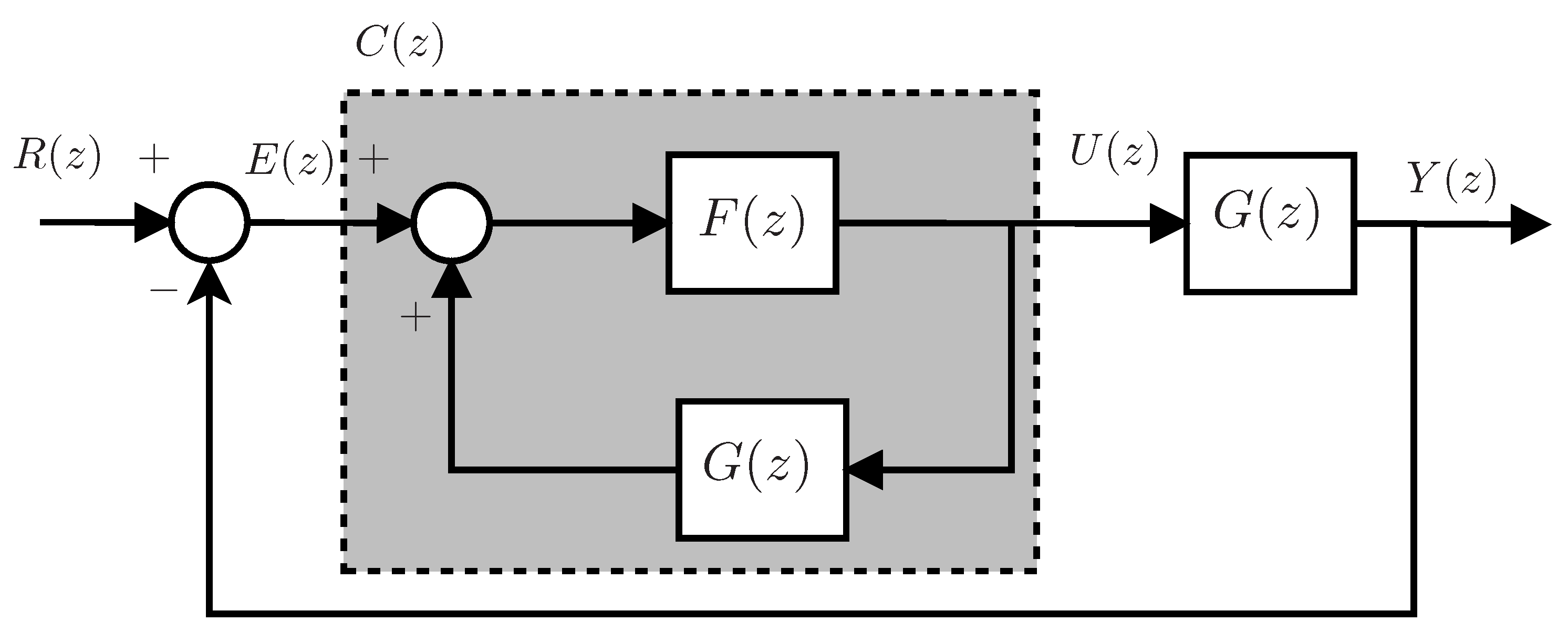
2.5. Repetitive Control Using the Stabilizing Controllers’ Parametrization

It is well known that all stabilizing controllers for a given plant, $G\left(z\right)$, can be written in terms of the Youla parametrization [27] shown in Figure 5. In this case, the sensitivity and complementary sensitivity functions are:

$$\begin{array}{ccc}\hfill S\left(z\right)& =& \frac{E\left(z\right)}{R\left(z\right)}=1-F\left(z\right)G\left(z\right)\hfill \end{array}$$

(26)

$$\begin{array}{ccc}\hfill T\left(z\right)& =& \frac{Y\left(z\right)}{R\left(z\right)}=F\left(z\right)G\left(z\right)\hfill \end{array}$$

(27)

where $F\left(z\right)$ is a stable system, and the controller is defined as $C\left(z\right)=\frac{U\left(z\right)}{E\left(z\right)}=\frac{F\left(z\right)}{1-F\left(z\right)G\left(z\right)}$.

In the case of minimum-phase plants, it is possible to select $F\left(z\right)=F^{\prime }\left(z\right)G^{-1}\left(z\right)$, so the closed-loop functions become:

$$\begin{array}{c}\hfill S\left(z\right)=\frac{E\left(z\right)}{R\left(z\right)}=1-F^{\prime }\left(z\right),T\left(z\right)=\frac{Y\left(z\right)}{R\left(z\right)}=F^{\prime }\left(z\right).\end{array}$$

(28)

In order to impose that the controller behaves as an RC, it is necessary to impose the appropriate shape for $F^{\prime }\left(z\right)$. It is necessary that:

$$S\left(z\right)=\frac{E\left(z\right)}{R\left(z\right)}=1-F^{\prime }\left(z\right)=\left(1-\sigma W\left(z\right)H\left(z\right)\right)\frac{N_s\left(z\right)}{D_s\left(z\right)}$$

(29)

with $N_s\left(z\right)$ and $D_s\left(z\right)$ arbitrary elements. Therefore,

$$F^{\prime }\left(z\right)=\frac{D_s\left(z\right)-\left(1-\sigma W\left(z\right)H\left(z\right)\right)N_s\left(z\right)}{D_s\left(z\right)}.$$

(30)

A simple solution is $N_s\left(z\right)=1$ and $D_s\left(z\right)=1-\alpha ·\sigma ·W\left(z\right)H\left(z\right)$ with $\left|\alpha \right|<1$, which generates:

$$F^{\prime }\left(z\right)=\frac{(1-\alpha )·\sigma ·W\left(z\right)H\left(z\right)}{1-\alpha ·\sigma ·W\left(z\right)H\left(z\right)}.$$

This option yields the following closed-loop transfer functions:

$$\begin{array}{ccc}\hfill T\left(z\right)& =& \frac{Y\left(z\right)}{R\left(z\right)}=\frac{(1-\alpha )·\sigma ·W\left(z\right)H\left(z\right)}{1-\alpha ·\sigma ·W\left(z\right)H\left(z\right)}\hfill \end{array}$$

(31)

$$\begin{array}{ccc}\hfill S\left(s\right)& =& \frac{E\left(z\right)}{R\left(z\right)}=\frac{1-\sigma ·W\left(z\right)H\left(z\right)}{1-\alpha ·\sigma ·W\left(z\right)H\left(z\right)},\hfill \end{array}$$

(32)

which can be considered a generalized version of the series approach (Section 2.2).

Finally, the robust stability condition for plants with multiplicative uncertainty is:

$${∥W_u^m\left(z\right)\frac{(1-\alpha )·\sigma ·W\left(z\right)H\left(z\right)}{1-\alpha ·\sigma ·W\left(z\right)H\left(z\right)}∥}_{\infty }<1.$$

(33)

Clearly, this approach can generate a more complex closed-loop transfer function; in particular, the closed-loop poles could be arbitrarily placed by choosing and appropriate value for $D_s\left(z\right)$. Alternatively, these degrees of freedom could be used to optimize any criteria such as robustness. This increment in controller complexity would increase the computational resources required to implement the controller.

2.6. $H_{\infty }$ Scheme

Previous approaches provided an analytic solution to the RC design by setting some of its parameters. A complementary strategy, which has been proposed in the literature [32,33], is to setup the controller by means of an $H_{\infty }$ optimal design.

Usually, the series architecture, introduced in Section 2.2, is taken as the implementation scheme, as shown in Figure 6. This design procedure allows us to take into account the plant uncertainty during the design procedure (in previous approaches, robustness could be tested once the controller was designed, using the robustness conditions). Consequently, the plant is described as a nominal plant, $G_n\left(z\right)$, and multiplicative weighting function, i.e., $G\left(z\right)=G_n\left(z\right)\left(1+W_u^m\left(z\right)\Delta \left(z\right)\right)$, with ${\parallel \Delta \left(z\right)\parallel }_{\infty }<1$.

In order to use $H_{\infty }$ design techniques, the problem needs to be appropriately formulated [27]. This means building an augmented plant, which also contains specification and uncertainty functions. The obtained controller has the order of this augmented plant. Including the RC internal model in the augmented plant would imply obtaining a very high order controller. Due to this, since the first work designed RC in the $H_{\infty }$ framework [34], the delay function, $W\left(z\right)$, included in the internal model has been taken out from the augmented plant.

The proposed augmented plant is shown in Figure 7, and the equations that describe it are the following:

$$\left[\begin{array}{c}{Y}_1\left(z\right)\\ Y_2\left(z\right)\\ Y_3\left(z\right)\end{array}\right]=P\left(z\right)\left[\begin{array}{c}{U}_1\left(z\right)\\ U_2\left(z\right)\\ U_3\left(z\right)\end{array}\right]$$

(34)

where:

$$P\left(z\right)=\left[\begin{array}{ccc}0& 0& W_u^m\left(z\right)\\ -\frac{H\left(z\right)}{z^h}{G}_n\left(z\right)& \frac{H\left(z\right)}{z^h}& -\frac{H\left(z\right)}{z^h}{G}_n\left(z\right)\\ 0& 1& 0\end{array}\right].$$

(35)

with $\xi$ being a design parameter used to add flexibility during the design [35]. Note that when building $P\left(z\right)$, $H\left(z\right)$ is made causal by including a number of delays equal to its relative degree, h; in the implementation, these delays are taken from the ones in $W\left(z\right)$.

The $H_{\infty }$-based design objective is to find a stabilizing controller $K\left(z\right)$ that minimizes the $H_{\infty }$ norm of system $M\left(z\right)=F_l(P\left(z\right),K\left(z\right))$ ($F_l(P\left(z\right),K\left(z\right))$ denotes the lower LFT (Linear Fractional Transformation) of $P\left(z\right)$ with respect to $K\left(z\right)$). In the case the transfer function from ${\left[U_1\left(z\right),U_2\left(z\right)\right]}^T$ to ${\left[Y_1\left(z\right),Y_2\left(z\right)\right]}^T$, i.e., $M\left(z\right)$, fulfills ${\parallel M\left(z\right)\parallel }_{\infty }<1$, robust stability will be guaranteed when $W\left(z\right)$ and $\Delta \left(z\right)$ are included in the diagram [32,33].

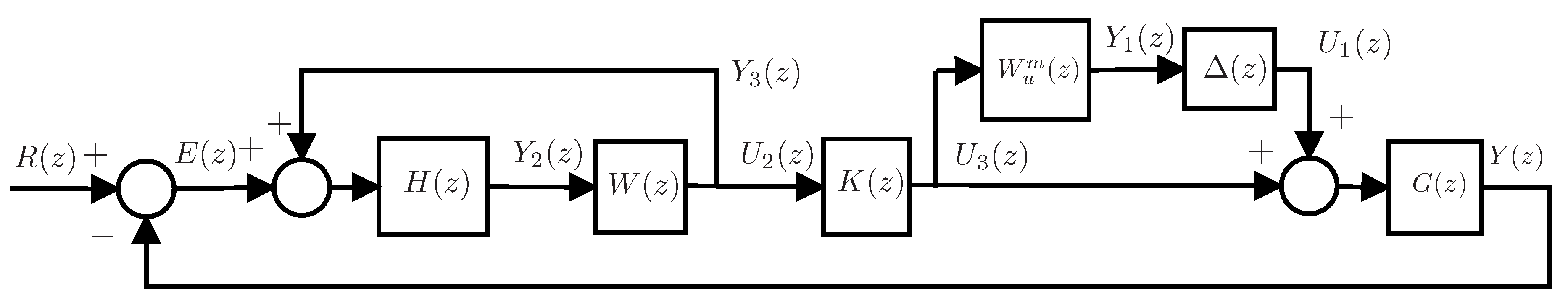
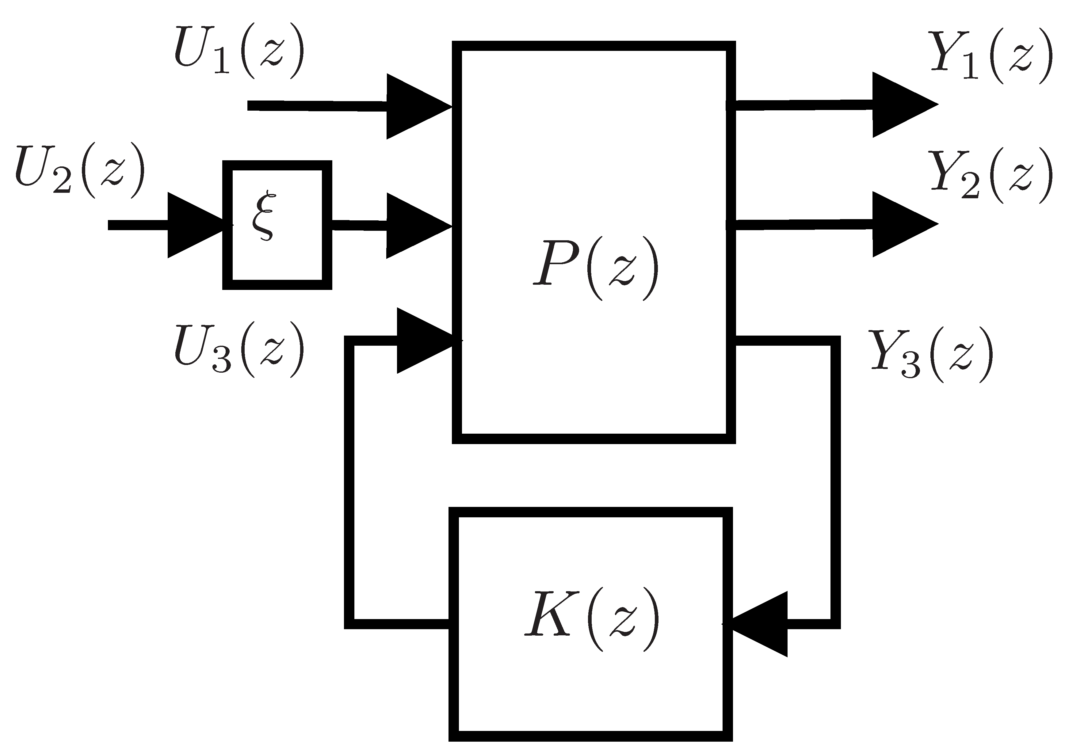
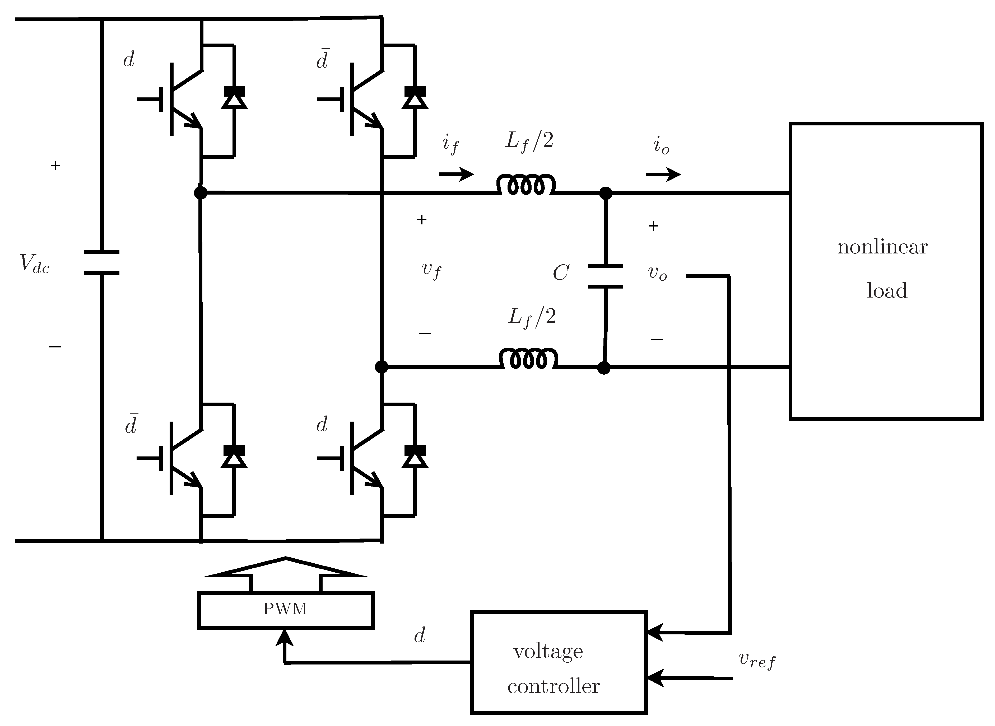
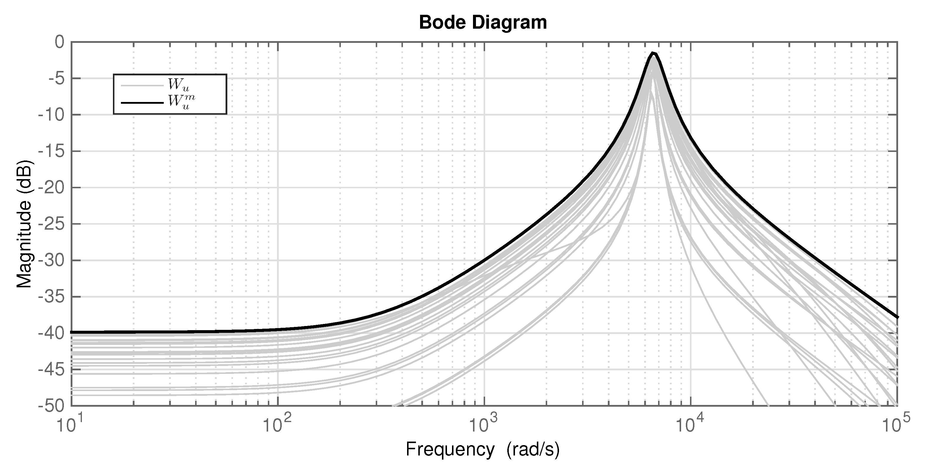
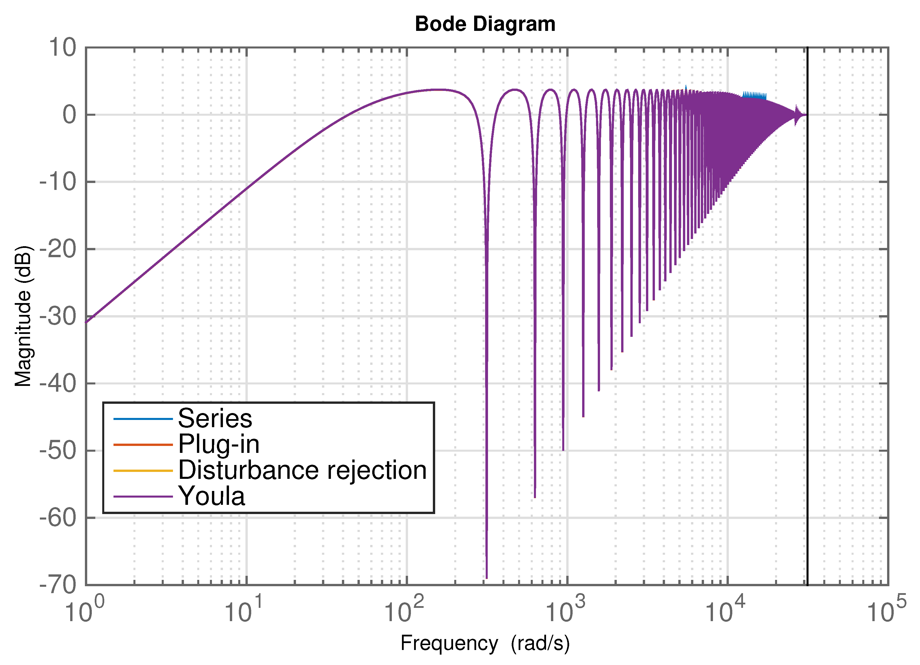
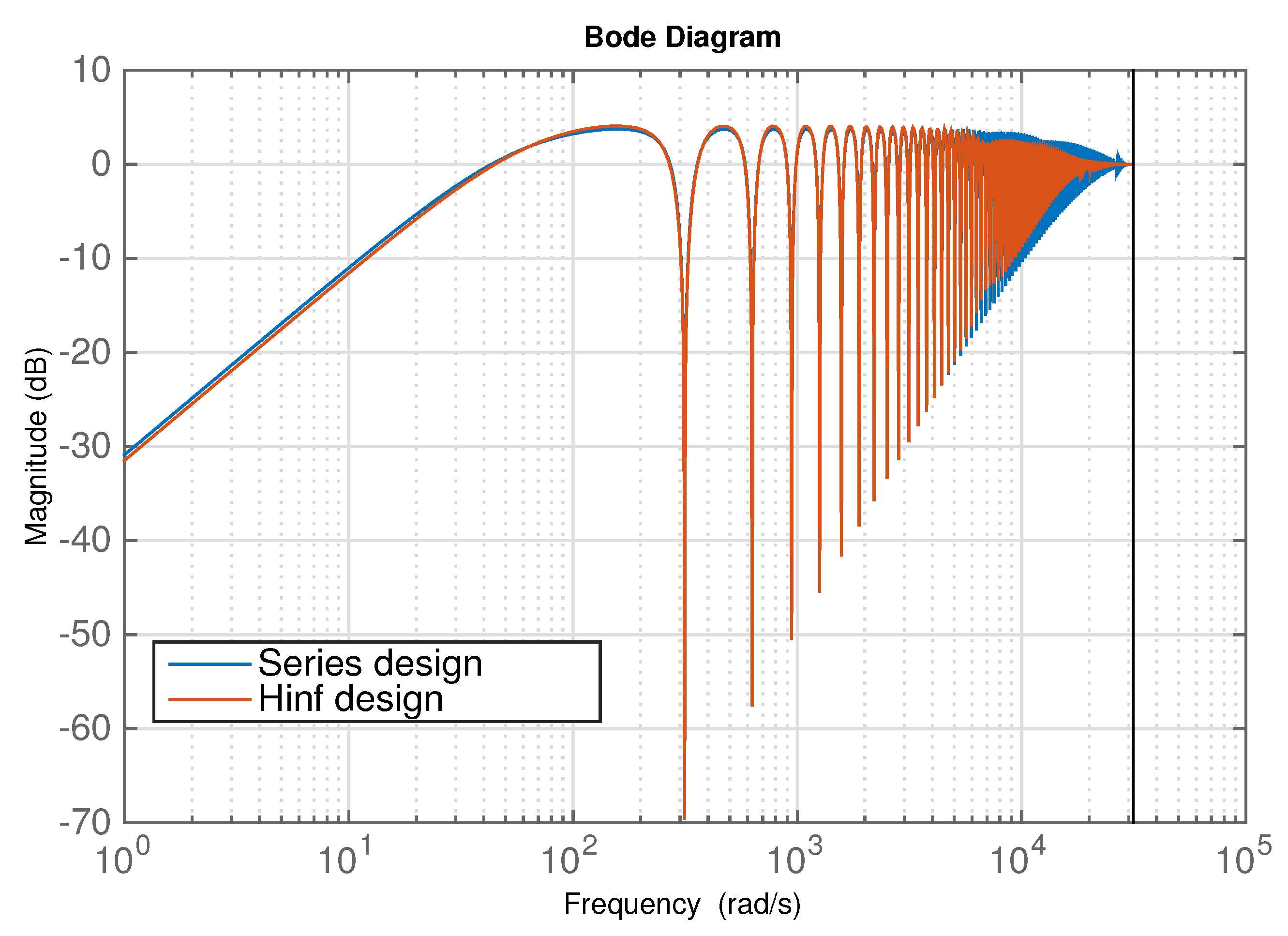
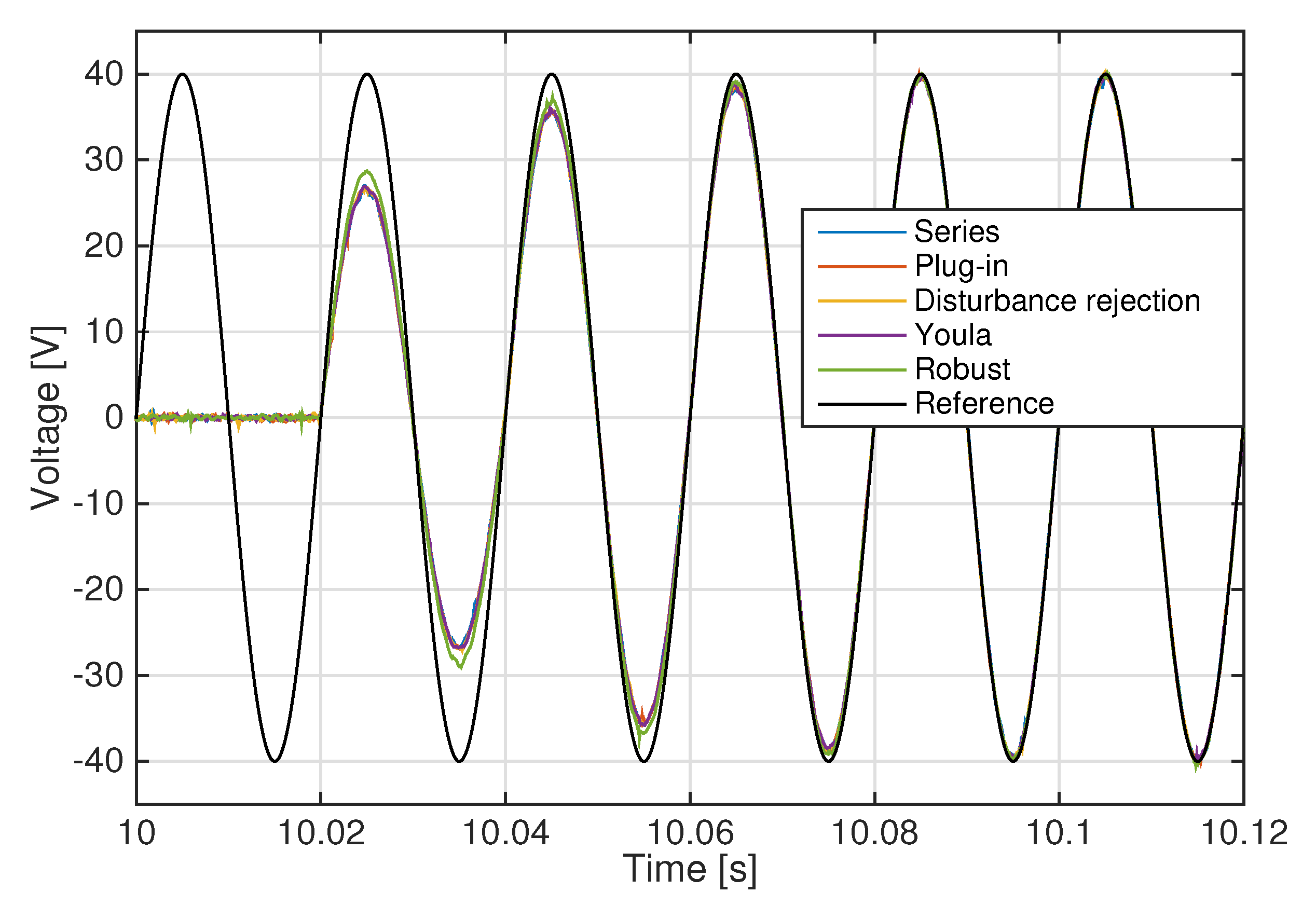
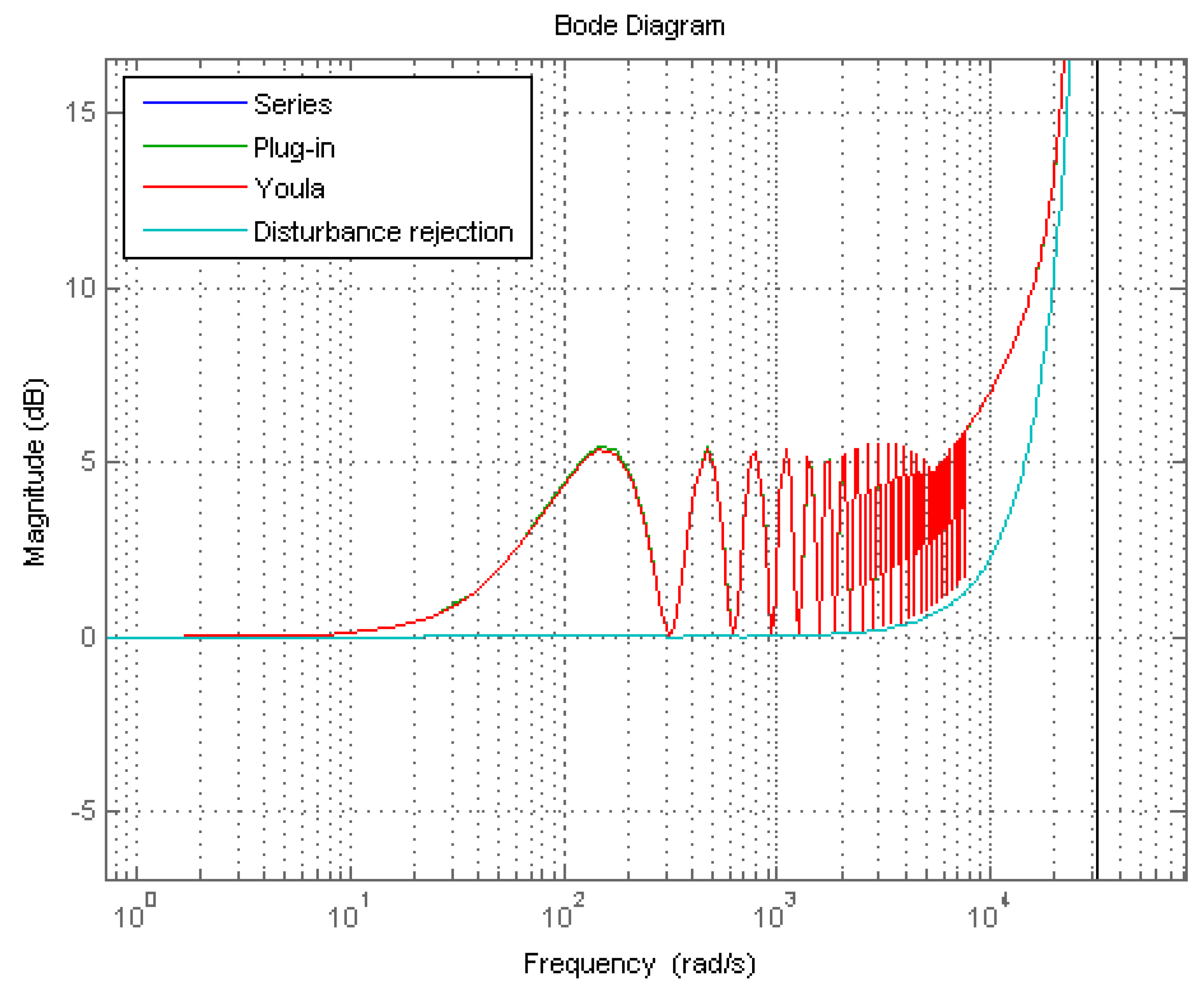
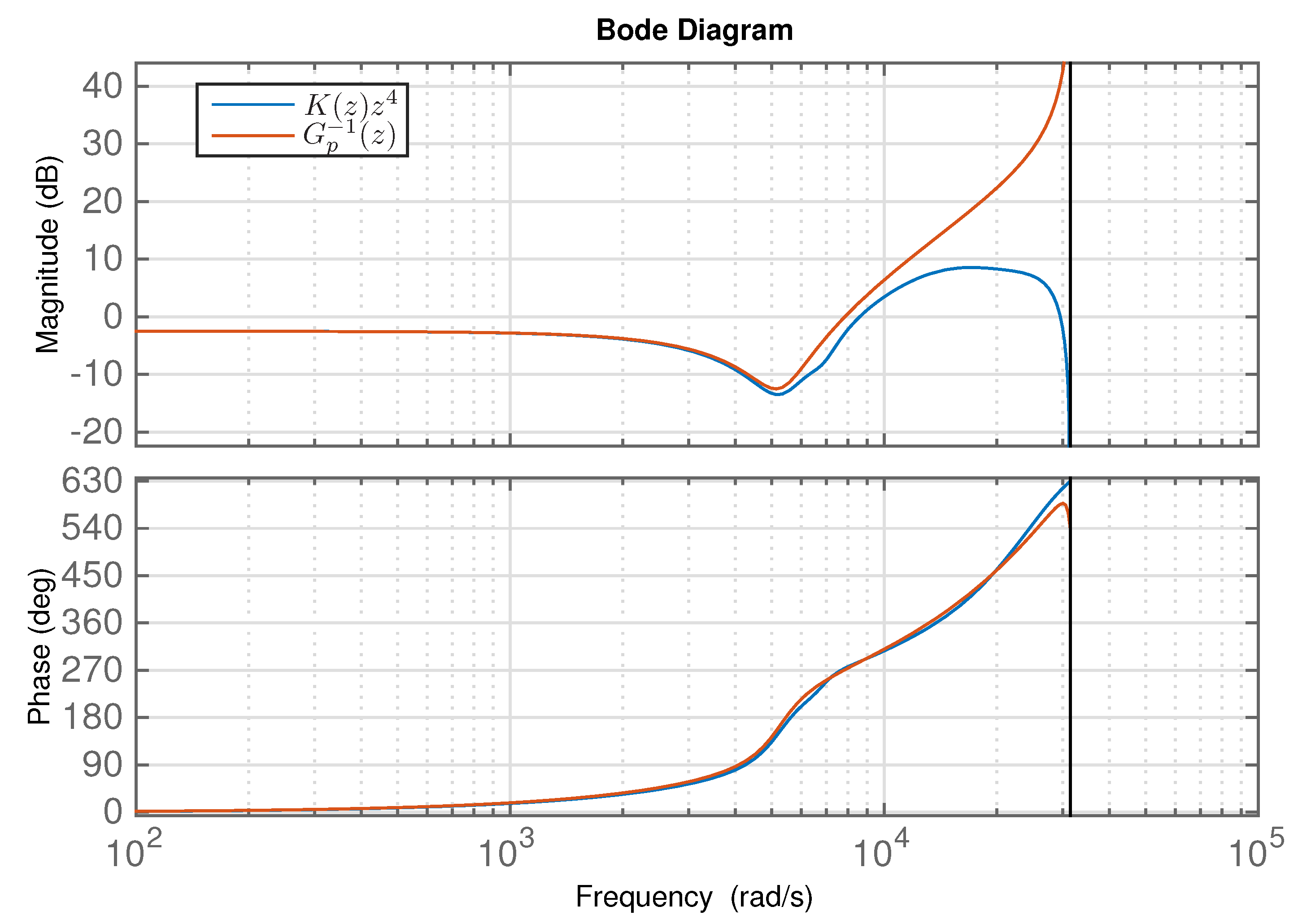
3. Repetitive Control Design for the Voltage Source Inverter

In this section, previously-introduced RC architectures will be used to design a control system for a VSI; which transforms a DC voltage source, $v_{dc}$, into an AC voltage source, $v_o$. The experimental setup is based on the system depicted in Figure 8. VSIs have become very popular in renewable energy systems, which are usually DC voltage sources [35], and Uninterruptible Power Supplies (UPS) [36].

VSIs are composed by a switching devices, i.e., IGBT, connected to the DC voltage source, $v_{dc}$, and governed by a Pulse Width Modulation (PWM) signal, with a given duty cycle, d; and a filter, an LC one in our case, whose main role is to low-pass filter the output of the switching devices. The main objective is generating a sinusoidal output voltage, $v_o$, with the desired amplitude and frequency ($v_{ref}$) [37]. In this work, $v_{ref}$ will be the sinusoidal voltage of frequency $f=50$ Hz and amplitude 40 V.

Usually, this output voltage, $v_o$, is used to feed different loads. These loads interfere with the filter dynamics; additionally, nonlinear loads introduce harmonics [35]. Rejecting the effect of these loads is a challenging control problem. RC is a control technique that can appropriately deal with this problem. A way of measuring the system performance is through the Total Harmonic Distortion (THD).

Figure 9 shows the experimental setup that will be used to validate the RC behavior. It is based on a Semikron configurable power stage, which has been used to reproduce the configuration shown in Figure 8.

The averaged behavior of the VSI, shown in Figure 8, can be described by the following equations in the Laplace domain:

$$V_o\left(s\right)=G_p\left(s\right)V_f\left(s\right)-G_d\left(s\right)I_o\left(s\right),$$

(36)

with:

$$G_p\left(s\right)=\frac{R_C}{L_{f}C{R}_C{s}^2+(C{R}_f{R}_C+L_f)s+(R_f+R_C)},$$

(37)

and:

$$G_d\left(s\right)=\frac{L_{f}s+R_f}{L_{f}C{R}_C{s}^2+(C{R}_f{R}_C+L_f)s+(R_f+R_C)},$$

(38)

where $G_p\left(s\right)$ is the plant transfer function; $G_d\left(s\right)I_o\left(s\right)$ is the disturbance signal caused by the load; $V_f\left(s\right)=(2d-1)V_{dc}$ is the control action where $d\in [0,1]$ is the PWM duty cycle and $V_{dc}$ is the DC voltage. The LC filter is composed of the inductance $L_f$ and capacitor C, and the series parasitic resistance of the inductance is $R_f$, while the parallel parasitic resistance of the capacitor is $R_C$. It is also useful to remark that $G_d\left(s\right)$ is actually the inverter output impedance.

In the VSI used in this work, the following values for the parameters have been used: $L_f=900\mu \mathrm{H}$, $C=40\mu \mathrm{F}$, $R_f=1.5\Omega$, and $R_C=8200\Omega$. The PWM signals have a switching frequency of 15 $\mathrm{kHz}$, and their duty cycle is updated each sampling time $T_s=0.0001\mathrm{s}$ is used.

As the signal to be tracked has a period of $T_p=\frac{1}{50}=0.02\mathrm{s}$ and the sampling time has been selected as $T_s=0.0001\mathrm{s}$, the discrete-time period becomes $N=T_p/T_s=200$.

In order to analyze the load impedance effect over the closed-loop system, it will be modeled as a dynamic uncertainty. The relationship between the output current, $i_o$ and the output voltage $v_o$ is given by: $I_o\left(s\right)=\frac{V_o\left(s\right)}{Z\left(s\right)}$, with $Z\left(s\right)$ being the load impedance. In this work, the load is modeled as an inductance and a resistor in series; under this assumption, the impedance can be computed as:

$$Z\left(s\right)=s{L}_L+R_L.$$

(39)

Therefore, for the complete system, converter low-pass filter plus the load impedance, the dynamic behavior can be modeled as:

$$G\left(s\right)=\frac{G_p\left(s\right)}{1+\frac{G_d\left(s\right)}{Z\left(s\right)}},$$

(40)

which can be rewritten as:

$$G\left(s\right)=G_p\left(s\right)\left(1-\frac{G_d\left(s\right)}{Z\left(s\right)+G_d\left(s\right)}\right).$$

As the load is assumed uncertain, this plant is modeled as a nominal plant, defined by $G_p\left(s\right)$ and a multiplicative uncertainty:

$$G\left(s\right)=G_p(1+W_u^m\left(s\right)\Delta \left(s\right)).$$

(41)

where $|W_u^m\left(j\omega \right)|$ corresponds to a bound on the maximum value of $\left|\frac{G_d\left(j\omega \right)}{Z\left(j\omega \right)+G_d\left(j\omega \right)}\right|$ at each frequency.

In this work, it is assumed that $R_L\in \left[10100\right]\Omega$ and $L_L\in \left[1010000\right]\mu H$. Figure 10 shows the frequency response of $\left|\frac{G_d\left(j\omega \right)}{Z\left(j\omega \right)+G_d\left(j\omega \right)}\right|$ for a number of possible loads. The figure shows also the frequency response of $|W_u^m\left(j\omega \right)|$, for:

$$W_u^m\left(z\right)=\frac{0.1269z^2-0.1219z-0.001209}{z^3-1.442z^2+0.865z}.$$

(42)

This transfer function, corresponding to an uncertainty bound, has been numerically obtained using the MATLAB Robust Toolbox.

Based on (41), different RC will be designed. An element present in all these architectures is the low-pass filter $H\left(z\right)$. This element’s most relevant goal is to introduce robustness in the high-frequency range. In this work, the following filter has been used:

$$H\left(z\right)=\frac{0.25z^2+0.5z+0.25}{z},$$

(43)

it has a null-phase, a gain close to one in the low- and medium-frequency range and an important attenuation in the high-frequency range. This is consistent with the uncertainty assumed in the load (Figure 10).

The series and plug-in structures, introduced in Section 2.2 and Section 2.3, respectively, have in $k_r$ a design parameter that is related to the closed-loop poles’ location. In this manner, these poles are approximately the solution of $z^N=1-k_r$. As a consequence, their location is distributed along a circle with the radius defined by $|1-k_r|$. This fact, in turn, defines the settling time in the closed-loop response [38,39]. Furthermore, a balance between robustness and settling time can be made through the selection of $k_r$. As a result, a value of $k_r=0.7$ is found to be suitable for the experiments.

Similar to parameter $k_r$, the disturbance rejection and Youla parametrization schemes (Section 2.4 and Section 2.5 respectively) use the parameter $\alpha$. Thus, $\alpha$ is also related to the closed-loop poles. In fact, these parameters are related in a straightforward fashion by means of the equation $\alpha =1-k_r$. The consequence is that, for all these architectures, we can achieve the same pole location using the appropriate value of $\alpha$. To be consistent with the value of $k_r$ previously selected, $\alpha =0.3$ is set.

An internal controller is used in the plug-in (Section 2.3) and disturbance rejection schemes (Section 2.4). This controller is designed to obtain good enough low-frequency response and robustness. A proportional compensator has been selected in order to provide a simple way to compare these controllers:

$$G_c\left(z\right)=0.002.$$

(44)

The design of the $H_{\infty }$ controller, introduced in Section 2.6, is made using $H\left(z\right)$ as described in (43) with $h=1$ for the construction of $P\left(z\right)$. The design also uses the previously-defined weighting function $W_u^m\left(z\right)$ and $\xi =100$. The MATLAB algorithm hinfsyn is employed to obtain the controller.

The frequency plot of the sensitivity function is shown in Figure 11 for the series, plug-in, disturbances observer, and Youla schemes. It can be observed that the frequency responses are practically the same and all systems will provide good harmonic rejection. The effect of the filter $H\left(z\right)$ can be seen as the attenuation of the harmonics at higher frequencies being decreased. In addition, the sensitivity function does not reach $6 \mathrm{dB}$, which is a good indicator of robustness.

Figure 12 shows the sensitivity function comparison for the $H_{\infty }$ and the series designs. As can be seen, at lower frequencies, the response is very similar, whilst the robust design achieves a smaller frequency response at higher frequencies, which is desirable to obtain a more robust controller.

The experimental closed-loop transient response is shown in Figure 13. For this experiment, a $50\mathrm{Hz}$ sinusoidal reference with $40 \mathrm{V}$ of amplitude is introduced at $t=10$ s. It can be seen that all controllers have almost the same transient response, except for the robust design, which is slightly faster. This small difference is a consequence of the equivalence of the obtained robust controller and a series design with $k_r=0.749$, as will be shown later.

The robustness against load uncertainty is analyzed using the multiplicative uncertainty $W_u^m\left(z\right)$ as a model of the system variations. The condition for robust stability is $\parallel W_u^m{\left(z\right)T\left(z\right)\parallel }_{\infty }<1$, which frequency by frequency can be analyzed as:

$$|W_u^m\left(e^{j\omega T_s}\right)|<\frac{1}{\left|T\right(e^{j\omega T_s}\left)\right|}.$$

(45)

The magnitude Bode plot of the function $T{\left(z\right)}^{-1}$ is shown in Figure 14. It can be observed that the plot remains over $0\mathrm{dB}$ for the entire frequency interval, and especially at high frequencies. As a result, all controllers can deal with a change of $100\%$ in the plant system at each frequency, which means that a good robustness characteristic has been obtained. Furthermore, as depicted in Figure 10, the gain of $W_u^m\left(s\right)$ is always lower than $0\mathrm{dB}$ for the selected load variation. This fact together with the previous analysis of Figure 14 demonstrate that all RC structures achieve good robust stability features.

On the other hand, the $H_{\infty }$ controller accomplishes the robust stability condition with ${∥W_u\left(z\right)T\left(z\right)∥}_{\infty }=0.628$. This means that the system achieves robust stability for the selected load variations. The bode plot of the obtained controller $K\left(z\right)$ and $k_r/G_p\left(z\right)$, with $k_r=0.749$, is shown in Figure 15.

Finally, with the $H_{\infty }$ design, the resulting controller achieves the robust stability condition with ${∥W_u\left(z\right)T\left(z\right)∥}_{\infty }=0.628$, which accomplishes the design criteria for the given load variations. Figure 15, shows the frequency response of $K\left(z\right)$ and $k_r/G_p\left(z\right)$, with $k_r=0.749$. It can be seen that the frequency response of $K\left(z\right)$ is very similar to the plant inverse for a large interval of frequencies. As reported in [40], it can be conjectured that the classical design of RC is close to an optimal one regarding robustness. Therefore, the $H_{\infty }$ design has very similar performance and robustness compared to the other presented RC configurations.

Finally, Figure 16 shows the experimental steady-state performance of the inverter for all the described architectures. In this experiment, a non-linear load is connected to the inverter and a non-sinusoidal current signal is produced, which introduces a disturbance with important harmonic content. The non-linear load consists of a full-bridge diode rectifier with a 470 $\mu$F capacitor on the DC side and a 9 $\Omega$ resistive load. Figure 16 depicts the effect of this disturbance in the voltage signal of the inverter measured through the Total Harmonic Distortion (THD). As can be seen, all strategies obtained very similar THD of around 1%. Furthermore, this figure shows the load current harmonic content, load power consumption, and detailed voltage and current waveforms. These additional data confirm that the obtained steady-state performance is very similar for all the strategies.

4. Conclusions

This work has reviewed, compared, and classified the most relevant z-transform-based architectures described in the literature to implement repetitive controllers. Concrete closed-loop expressions have been introduced, using a homogeneous notation, for the most relevant closed-loop transfer functions and robust stability conditions for generic discrete time minimum-phase plants. The equivalence between all architectures has been established under appropriate parameter selection. All these architectures have been used to design a VSI control system, and experimental and simulation results have been shown in the paper.

Based on the developments and experimental results, all architectures achieved similar steady-state behavior. This steady-state behavior depends only on the generator. As all the architectures include the same generator, it is logical that all offer the same steady-state error. All architectures use the FIR low-pass filter to improve the closed-loop robustness. It must be designed using a trade-off between the desired performance and the reached robustness, i.e., the filter reduces the gain at harmonic frequencies, so steady-state error is increased. This filter affects all the architectures equally; therefore, there is no difference between them in this regard.

The plug-in and disturbance observer architectures use an internal controller, $G_c$, which can be used to improve the transient behavior and robustness of the closed-loop system. Unfortunately, this element introduces additional complexity in the design, and there are no clear criteria for the design; so, in general, most people tend to use a proportional controller. On the contrary, the series approach offers a very straightforward design with less degrees of freedom.

The Youla parametrization approach offers a very generic methodology allowing us to include new specifications. Unfortunately, this architecture is not used much in practice due to the important increase in the required computational burden (the controller is more complex). Developing methodologies that allow profiting from this flexibility while preserving a limited computational burden is a challenge, which is being addressed by several researchers.

Finally, robust and optimal designs based on tools like the $H_{\infty }$ approach provide another option for tuning RC controllers. This approach is the only one that allows taking into account the uncertainty during the controller design; in the other approaches, only robustness testing is feasible; consequently, if uncertainty is very relevant in the system, this would be the best option. Some relevant aspects, such as avoiding the high order delay of the internal model, should be taken into account to obtain a suitable design. Although using this approach provides an advanced design methodology and achieves optimal performance, according to our experience, the improvement is not much in practice. An open topic in this approach is the simultaneous co-design of the controller and the low-pass filter, the main objective of which is dealing with uncertainty. Current approaches fix the low-pass filter a priori and design the controller later. A co-design would, for sure, provide better results.

From our point of view, the plug-in architecture is, in general, the most convenient one. It offers nice results with quite a straightforward algorithm. In some systems, the disturbance estimation can be used for online analysis of fault detection. In those cases, the disturbance rejection methodology might be of more interest. Finally, in a system subject to an important uncertainty, the $H_{\infty }$ approach would be the most relevant one.

References

1. Wang, Y.; Gao, F.; Doyle, F.J. Survey on iterative learning control, repetitive control, and run-to-run control. J. Process Control 2009, 19, 1589–1600. [Google Scholar] [CrossRef]
2. Longman, R.W. Iterative learning control and repetitive control for engineering practice. Int. J. Control 2010, 73, 930–954. [Google Scholar] [CrossRef]
3. Chen, Y.; Moore, K.L.; Yu, J.; Zhang, T. Iterative learning control and repetitive control in hard disk drive industry—A tutorial. Int. J. Adapt. Control Signal Process. 2008, 22, 325–343. [Google Scholar] [CrossRef]
4. Ahn, H.S.; Chen, Y.Q.; Moore, K.L. Iterative Learning Control: Brief Survey and Categorization. IEEE Trans. Syst. Man Cybern. Part C 2007, 37, 1099–1121. [Google Scholar] [CrossRef] [Green Version]
5. Álvarez, J.D.; Costa-Castelló, R.; Castilla, M.d.M. Repetitive Control to Improve Users’ Thermal Comfort and Energy Efficiency in Buildings. Energies 2018, 11, 976. [Google Scholar] [CrossRef]
6. Francis, B.; Wonham, W. The internal model principle of control theory. Automatica 1976, 12, 457–465. [Google Scholar] [CrossRef]
7. Costa-Castelló, R.; Olm, J.M.; Vargas, H.; Ramos, G.A. An Educational Approach To The Internal Model Principle For Periodic Signals. Int. J. Innov. Comput. Inf. Control 2012, 8, 5591–5606. [Google Scholar]
8. Ramos, G.; Costa-Castelló, R.; Olm, J.M. Digital Repetitive Control under Varying Frequency Conditions; Lecture Notes in Control and Information Sciences; Springer: Berlin/Heidelberg, Germany, 2013; Volume 446, ISBN 978-3-642-37778-5. [Google Scholar]
9. Park, S.W.; Jeong, J.; Yang, H.S.; Park, Y.P.; Park, N.C. Repetitive controller design for minimum track misregistration in hard disk drives. IEEE Trans. Magn. 2005, 41, 2522–2528. [Google Scholar] [CrossRef]
10. Inoue, T.; Nakano, M.; Kubo, T.; Matsumoto, S.; Baba, H. High Accuracy control of a proton syncrotron magnet powe supply. In Proceedings of the 8th Triennial World Congress of the International Federation of Automatic Control; IFAC by Pergamon Press: Tarrytown, NY, USA, 1982; pp. 3137–3142. [Google Scholar]
11. Ramos, G.A.; Costa-Castelló, R. Optimal anti-windup synthesis for repetitive controllers. J. Process Control 2013, 23, 1149–1158. [Google Scholar] [CrossRef]
12. Wang, L. Tutorial review on repetitive control with anti-windup mechanisms. Annu. Rev. Control 2016, 42, 332–345. [Google Scholar] [CrossRef]
13. Chen, X.; Tomizuka, M. New Repetitive Control With Improved Steady-State Performance and Accelerated Transient. IEEE Trans. Control Syst. Technol. 2014, 22, 664–675. [Google Scholar] [CrossRef]
14. Chen, X.; Tomizuka, M. Overview and new results in disturbance observer based adaptive vibration rejection with application to advanced manufacturing. Int. J. Adapt. Control Signal Process. 2015, 29, 1459–1474. [Google Scholar] [CrossRef]
15. Wu, M.; Xu, B.; Cao, W.; She, J. Aperiodic Disturbance Rejection in Repetitive-Control Systems. IEEE Trans. Control Syst. Technol. 2014, 22, 1044–1051. [Google Scholar]
16. Zhou, L.; She, J.; Wu, M.; He, Y. Design of a robust observer-based modified repetitive-control system. ISA Trans. 2013, 52, 375–382. [Google Scholar] [CrossRef] [PubMed]
17. Wu, M.; Zhou, L.; She, J. Design of Observer-Based H Robust Repetitive-Control System. IEEE Trans. Autom. Control 2011, 56, 1452–1457. [Google Scholar] [CrossRef]
18. Albalawi, H.; Zaid, S.A. An H5 Transformerless Inverter for Grid Connected PV Systems with Improved Utilization Factor and a Simple Maximum Power Point Algorithm. Energies 2018, 11, 2912. [Google Scholar] [CrossRef]
19. Rubio, F.R.; Navas, S.J.; Ollero, P.; Lemos, J.M.; Ortega, M.G. Control Óptimo Aplicado a Campos de Colectores Solares Distribuidos. Rev. Iberoam. Autom. Inf. Ind. 2018, 15, 327–338. [Google Scholar] [CrossRef]
20. Griñó, R.; Costa-Castelló, R. Digital repetitive plug-in controller for odd-harmonic periodic references and disturbances. Automatica 2005, 41, 153–157. [Google Scholar] [CrossRef]
21. Steinbuch, M.; Weiland, S.; Singh, T. Design of Noise and Period-Time Robust High Order Repetitive Control, with application to optical storage. Automatica 2007, 43, 2086–2095. [Google Scholar] [CrossRef]
22. Ramos, G.A.; Costa-Castelló, R. Power factor correction and harmonic compensation using second-order odd-harmonic repetitive control. IET Control Theory Appl. 2012, 6, 1–12. [Google Scholar] [CrossRef]
23. Escobar, G.; Hernandez-Briones, P.; Torres-Olguin, R.; Valdez, A. A repetitive-based controller for the compensation of 6l ± 1 harmonic components. In Proceedings of the IEEE International Symposium on Industrial Electronics, Vigo, Spain, 4–7 June 2007; pp. 3397–3402. [Google Scholar]
24. Escobar, G.; Mattavelli, P.; Hernandez-Gomez, M.; Martinez-Rodriguez, P.R. Filters With Linear-Phase Properties for Repetitive Feedback. IEEE Trans. Ind. Electron. 2014, 61, 405–413. [Google Scholar] [CrossRef]
25. Ye, Y.; Tayebi, A.; Liu, X. All-pass filtering in iterative learning control. Automatica 2009, 45, 257–264. [Google Scholar] [CrossRef]
26. Tomizuka, M. Zero Phase Error Tracking Algorithm for Digital Control. J. Dyn. Syst. Meas. Control 1987, 109, 65–68. [Google Scholar] [CrossRef]
27. Sánchez-Peña, R.S.; Sznaier, M. Robust Systems Theory and Applications; Adaptive and Learning Systems for Signal Processing, Communications and Control Series; Wiley-Interscience: Hoboken, NJ, USA, 1998. [Google Scholar]
28. Songschon, S.; Longman, R.W. Comparison of the stability boundary and the frequency response stability condition in learning and repetitive control. Int. J. Appl. Math. Comput. Sci. 2003, 13, 169–177. [Google Scholar]
29. Chen, W.H.; Yang, J.; Guo, L.; Li, S. Disturbance-Observer-Based Control and Related Methods: An Overview. IEEE Trans. Ind. Electron. 2016, 63, 1083–1095. [Google Scholar] [CrossRef]
30. Chen, X.; Tomizuka, M. An enhanced repetitive control algorithm using the structure of disturbance observer. In Proceedings of the 2012 IEEE/ASME International Conference on Advanced Intelligent Mechatronics (AIM), Kaohsiung, Taiwan, 11–14 July 2012; pp. 490–495. [Google Scholar]
31. Tang, M.; Formentini, A.; Odhano, S.; Zanchetta, P. Design of a repetitive controller as a feed-forward disturbance observer. In Proceedings of the IECON 2016—42nd Annual Conference of the IEEE Industrial Electronics Society, Florence, Italy, 24–27 October 2016; pp. 78–83. [Google Scholar]
32. Weiss, G.; Häfele, M. Repetitive control of MIMO systems using Hinfty design. Automatica 1999, 35, 1185–1199. [Google Scholar] [CrossRef]
33. Hornik, T.; Zhong, Q.C. A Current-Control Strategy for Voltage-Source Inverters in Microgrids Based on Hinfty and Repetitive Control. IEEE Trans. Power Electron. 2011, 26, 943–952. [Google Scholar] [CrossRef]
34. Wang, Y.; Wang, D.; Wang, X. A three-step design method for performance improvement of robust repetitive control. In Proceedings of the 2005 American Control Conference, Portland, OR, USA, 8–10 June 2005; Volume 2, pp. 1220–1225. [Google Scholar]
35. Hornik, T.; Zhong, Q.C. H repetitive voltage control of gridconnected inverters with a frequency adaptive mechanism. IET Power Electron. 2010, 3, 925–935. [Google Scholar] [CrossRef]
36. Deng, H.; Oruganti, R.; Srinivasan, D. Analysis and Design of Iterative Learning Control Strategies for UPS Inverters. IEEE Trans. Ind. Electron. 2007, 54, 1739–1751. [Google Scholar] [CrossRef]
37. Yang, Y.; Zhou, K.; Lu, W. Robust repetitive control scheme for three-phase constant-voltage-constant-frequency pulse-widthmodulated inverters. IET Power Electron. 2012, 5, 669–677. [Google Scholar] [CrossRef]
38. Yeol, J.W.; Longman, R.W.; Ryu, Y.S. On the Settling Time in Repetitive Control Systems. IFAC Proc. Vol. 2008, 41, 12460–12467. [Google Scholar] [CrossRef]
39. Garimella, S.; Srinivasan, K. Transient response of repetitive control systems. In Proceedings of the American Control Conference, Baltimore, MD, USA, 29 June–1 July 1994; pp. 2909–2913. [Google Scholar]
40. Ramos, G.A.; Costa-Castelló, R.; Olm, J.M. Analysis and design of a robust odd-harmonic repetitive controller for an active filter under variable network frequency. Control Eng. Pract. 2012, 20, 895–903. [Google Scholar] [CrossRef]
Figure 1. Generic periodical signal generator.
Electronics 07 00446 g001
Figure 2. Repetitive controller: series architecture block scheme.
Electronics 07 00446 g002
Figure 3. Repetitive controller: plug-in approach.
Electronics 07 00446 g003
Figure 4. Repetitive control: disturbance rejection-based approach.
Electronics 07 00446 g004
Figure 5. Repetitive control scheme: Youla parametrization approach.
Electronics 07 00446 g005
Figure 6. RC: series approach H design scheme.
Electronics 07 00446 g006
Figure 7. H design scheme.
Electronics 07 00446 g007
Figure 8. Voltage source inverter schematic diagram.
Electronics 07 00446 g008
Figure 9. Laboratory view of the voltage source inverter used to perform the experiments.
Electronics 07 00446 g009
Figure 10. Magnitude Bode diagram of W u = G d ( s ) Z ( s ) + G d ( s ) for different load values: R L [ 10 100 ] Ω and L L [ 10 10000 ] μ H , W u ( s ) , and the frequency response of the bounding function W u m ( s ) .
Electronics 07 00446 g010
Figure 11. Sensitivity function for RC based on the series, plug-in, disturbances observer, and Youla approaches.
Electronics 07 00446 g011
Figure 12. Sensitivity function comparison for RC based on the series and H approaches.
Electronics 07 00446 g012
Figure 13. Transient response for all approaches.
Electronics 07 00446 g013
Figure 14. Bode magnitude diagram of 1 / T ( z ) for all four approaches.
Electronics 07 00446 g014
Figure 15. Frequency response of K ( z ) obtained with the H design scheme.
Electronics 07 00446 g015
Figure 16. Experimental results for the nonlinear load. From top to bottom: series, plug-in, disturbance rejection, Youla, and robust designs. From left to right: voltage and load current wave forms, voltage harmonics, current harmonics, and power.
Electronics 07 00446 g016