1. Introduction
Vehicle detection is an essential and pivotal role in several applications like intelligent video surveillance [
1,
2,
3,
4], car crash analysis [
5], autonomous vehicle driving [
6]. Most traditional approaches adopt the way that the camera is installed on a low-altitude pole or mounted on the vehicle itself. For instance, Sun and Zehang [
7] present a method which jointly uses Gabor filters and Support Vector Machines for on-road vehicle detection. The Gabor filters are for feature extraction and these extracted features are used to train a classifier for detection. The authors in [
8] propose a method to detect vehicles from stationary images using colors and edges. Zhou, Jie and Gao [
9] propose a moving vehicle detection method based on example-learning. With regard to these approaches, the coverage of camera is limited despite rotating in multiple directions, they only detect vehicles on a small scale.
Given the installed camera’s limited coverage, researchers turn to other moving platforms. Satellites [
10,
11], aircrafts, helicopters and unmanned aerial vehicles have been used to solve the bottleneck. The cost of images collected by the satellites, aircrafts and helicopters is remarkably high, and this equipment isn’t able to make a quick response according to the time and weather. With the rapid development of the unmanned aerial vehicles industry, the price of small drones has dropped in recent years. The UAVs(unmanned aerial vehicles) have been the research focus. It seems easily accessible for the general public to obtain it, so all kinds of cameras including optical and infrared, have started to be installed on it. In this way, the unmanned aerial vehicle can be used as a height–adjustable moving camera platform on a large scale. Many researchers have made great efforts in this field. For example, Luo and Liu [
12] propose an efficient static vehicle detection framework on aerial range data provided by the unmanned aerial vehicle, which is composed of three modules–moving vehicle detection, road area detection and post processing. The authors in [
13] put forward a vehicle detection method from UAVs, which is integrated with Scalar Invariant Feature Transform and Implicit Shape Model. Another work [
14], a hybrid vehicle detection method that integrates the Viola–Jones (V–J) and linear SVM classifier with HOG(Histogram of Oriented Gradient) features, is proposed for vehicle detection for aerial vehicle images obtained in low-altitude. It is not able to choose a robust feature to aim at the small size vehicles. Besides, some researchers in [
15,
16,
17] have adopted the other sensors (e.g., depth sensors, RGB-D imagery) into the object detection area.
Another vehicle detection methods are accomplished by background modeling or foreground segmentation. The authors in [
18] put forward with a method of moving object detection on non–stationary cameras and bring it to vehicle detection on mobile device. They model the background through dual-mode single Gaussian Model with life–cycle model and compensate the motion of the camera via mixing neighboring models. The authors in [
19,
20] propose a method of detecting and locating moving object under realistic condition based on the motion history images representation, which incorporates the timed–MHI for motion trajectory representation. Afterwards, a spatio–temporal segmentation procedure is employed to label motion regions by estimating density gradient. However these methods might cause a great number false alarms and fail to detect the stationary vehicles.
All these adaptive detection methods above are same in essentials while differing in minor points. They employ the similar strategy: manual designed features (e.g., SIFT, SURF, HOG, Edge, Color or their combinations) [
21,
22,
23], background modeling or foreground segmentation, common classifiers (e.g., SVM, Adaboost) and sliding window search. These manual features might not hold the diversity of vehicles’ shapes, illumination variations and background changes. The sliding window is an exhaustive traversal, which is time–consuming, not purposeful. This might cause too many redundant bounding boxes and has a bad influence on the following extraction and classification’s speed and efficiency.
However, deep learning [
24,
25,
26,
27,
28,
29] establishes convolutional neural network that could automatically extract abundant representative features from the vast training samples. It has an outstanding performance on diverse data. Lars et al. [
25] propose a network for vehicle detection in aerial images, which has overcome the shortcoming of original approach in case of handling small instances. Deng et al. [
26] propose a fast and accurate vehicle detection framework, they develop an accurate–vehicle– proposal–network based on hyper feature map and put forward with a coupled R-CNN(convolutional neural network) method. A novel double focal loss convolutional neural network is proposed in [
27]. In this paper, the skip connection is used in the CNN structure to enhance the feature learning and the focal loss function is used to substitute for conventional cross entropy loss function in both the region proposed network and the final classifier. They [
27,
30,
31] all adopt the same framework, Region Proposal plus Convolutional Neural Network. By virtue of the CNN’s strong feature extraction capacity, it achieves a higher detection ratio. Inspired by these work above, the authors in [
29,
32] introduce the elementary framework on aerial vehicle detection and recognition. As described in [
29], a deep convolutional neural network is adopted to mine highly descriptive features from candidate bounding boxes, then a linear support vector machine is employed to classify the region into “car” or “no–car” labels. The authors in [
32] propose a hyper region proposal network to extract potential vehicles with a combination of hierarchical feature maps, then a cascade of boosted classifiers are employed to verify the candidate regions, false alarm ratio is further reduced.
All these work above have achieved tremendous advances in vehicle detection [
33,
34]. For object detection, images matching plays a vital role in searching part. The authors in [
33] propose a novel visible-infrared image matching algorithm, and they construct a co–occuring feature by cross-domain image database and feature extraction. Jing et al. [
34] extend the visible–infrared matching to photo-to-sketch matching by constructing visual vocabulary translator. The authors in [
15] extract object silhouettes from the noisy background by a sequence of depth maps captured by a RGB-D sensor and track it using temporal motion information from each frame. The authors in [
17] present a novel framework of 3D object detection, tracking and recognition from depth video sequences using spatiotemporal features and modified HMM. They use spatial depth shape features and temporal joints features to improve object classification performance. However, those approaches are not suitable for aerial infrared vehicle detection. The vehicle detections based on deep neural network and classification can’t reach the real-time demands. The vehicle detections based on these manual designed features’ matching have poor performances on the detection ratio measurement, for the aerial infrared images are low resolution and fuzzy and the manually extracted features are rare.
Considering the trade-off between the real-time demand and quantified index–
,
and
-
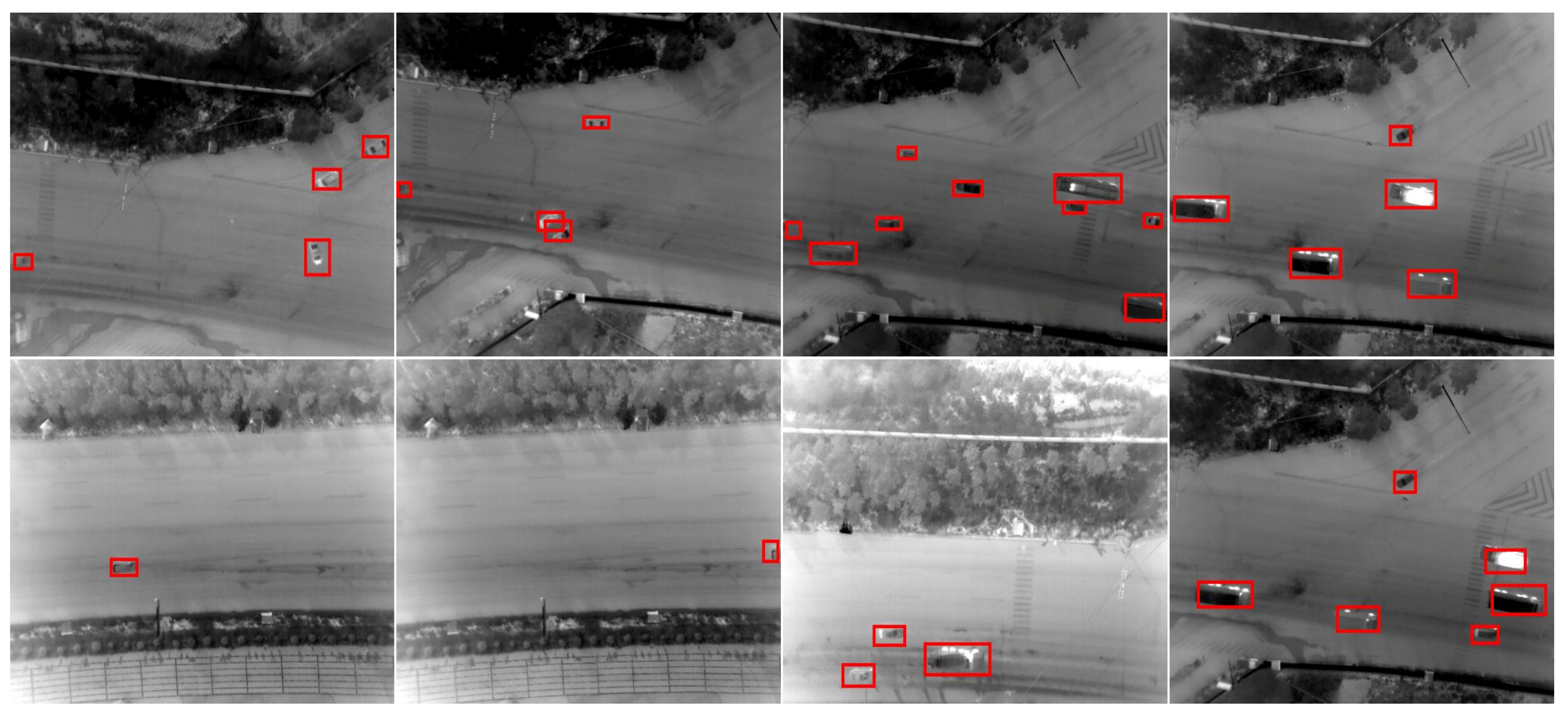
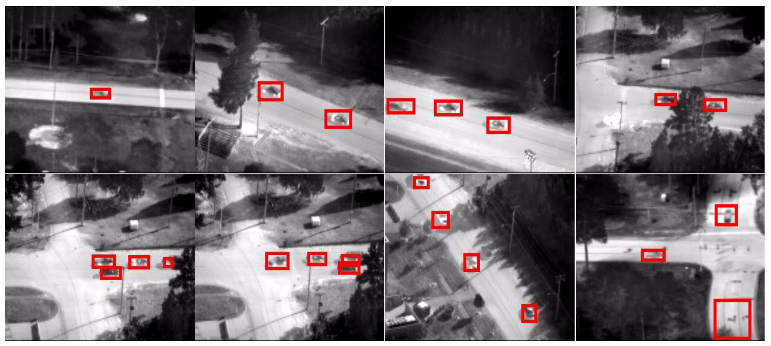
, we adopt the convolutional neural network (the number of layers is not deep) to extract abundant features in the aerial infrared images, treat the vehicle detection as a typical regressive problem to accelerate the bounding boxes generations. Some detection results are illustrated in
Figure 1. The majority of vehicles are detected, and these bounding boxes approximately cover the vehicles. The proposed method unexpectedly runs at a sampling frequency of 10 fps. The real-time vehicle detection is demanding. In the detection system, we might not demand an extremely accurate vehicle position, but an approximate position obtained in time is more necessary. Once detection speed falls behind the sample frequency, the information provided is lagged. This might mislead surveillance system.
The main contributions of this paper can be summarized as follows:
We propose a method of detecting ground vehicles in aerial imagery based on convolutional neural network. Firstly, we combine the UAV and infrared sensor to the real-time system. There exist some great challenges like scale, view changes and scene’s complexity in ground vehicle detection. In addition, the aerial imagery is always low-resolution, fuzzy and low-contrast, which adds difficulties to this problem. However, the proposed method adopts a convolutional neural network instead of traditional feature extraction, and uses the more recognized abstract features to search the vehicle, which have the unique ability to detect both the stationary and moving vehicles. It can work in real urban environments at 10 fps, which has a better real-time performance. Compared to the mainstream background model methods, it gets double performances in the and index.
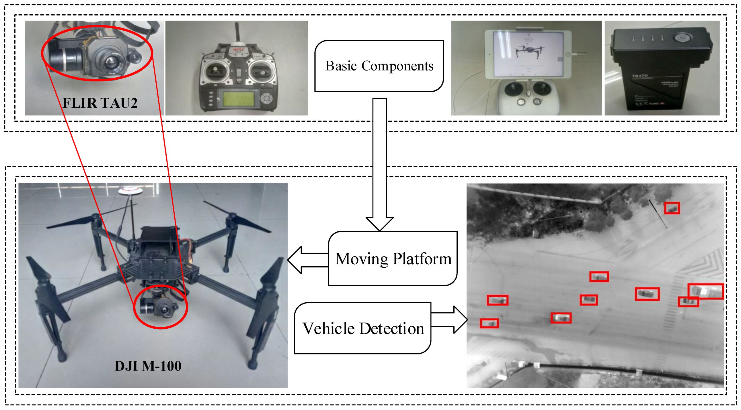
We construct a real-time ground vehicle detection system in aerial imagery, which includes the DJI M-100 UAV (Shenzhen, China), the FLIR TAU2 infrared camera (Beijing, China.), the remote controls and iPad (Apple, California, US). The system is built to collect large amounts of training samples and test images. These images are captured on different scenes includes road and multi-scenes. Additionally, this dataset is more complex and diversified in vehicle number, shape and surroundings. The aerial infrared vehicle dataset (The dataset (NPU_CS_UAV_IR_DATA) is online at [
35],) which is convenient for the future research in this field.
2. Aerial Infrared Ground Vehicle Detection
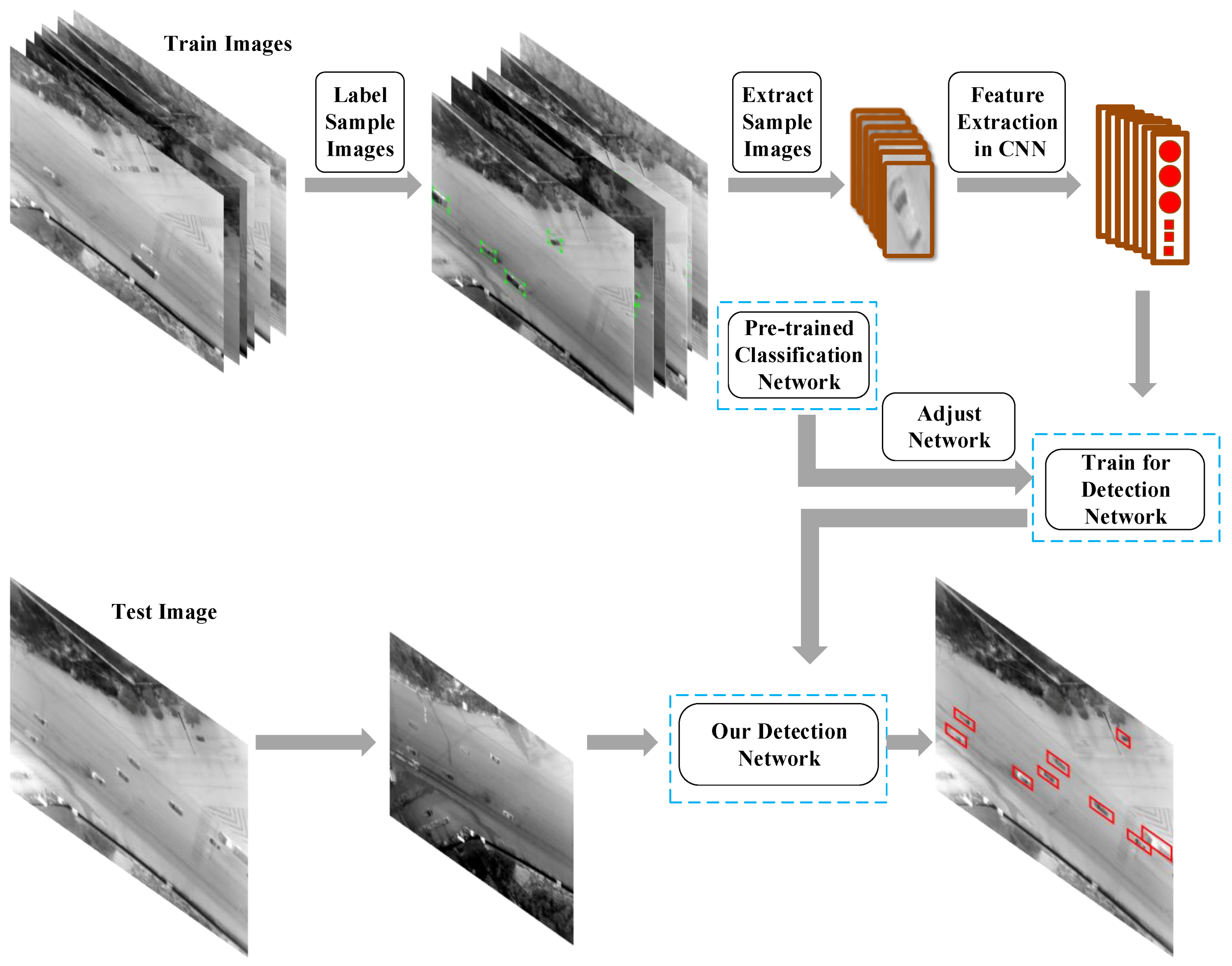
The proposed method is illustrated in
Figure 2. It can be mainly divided into three steps. First, we manually segment vehicles by the help of a
toolbox [
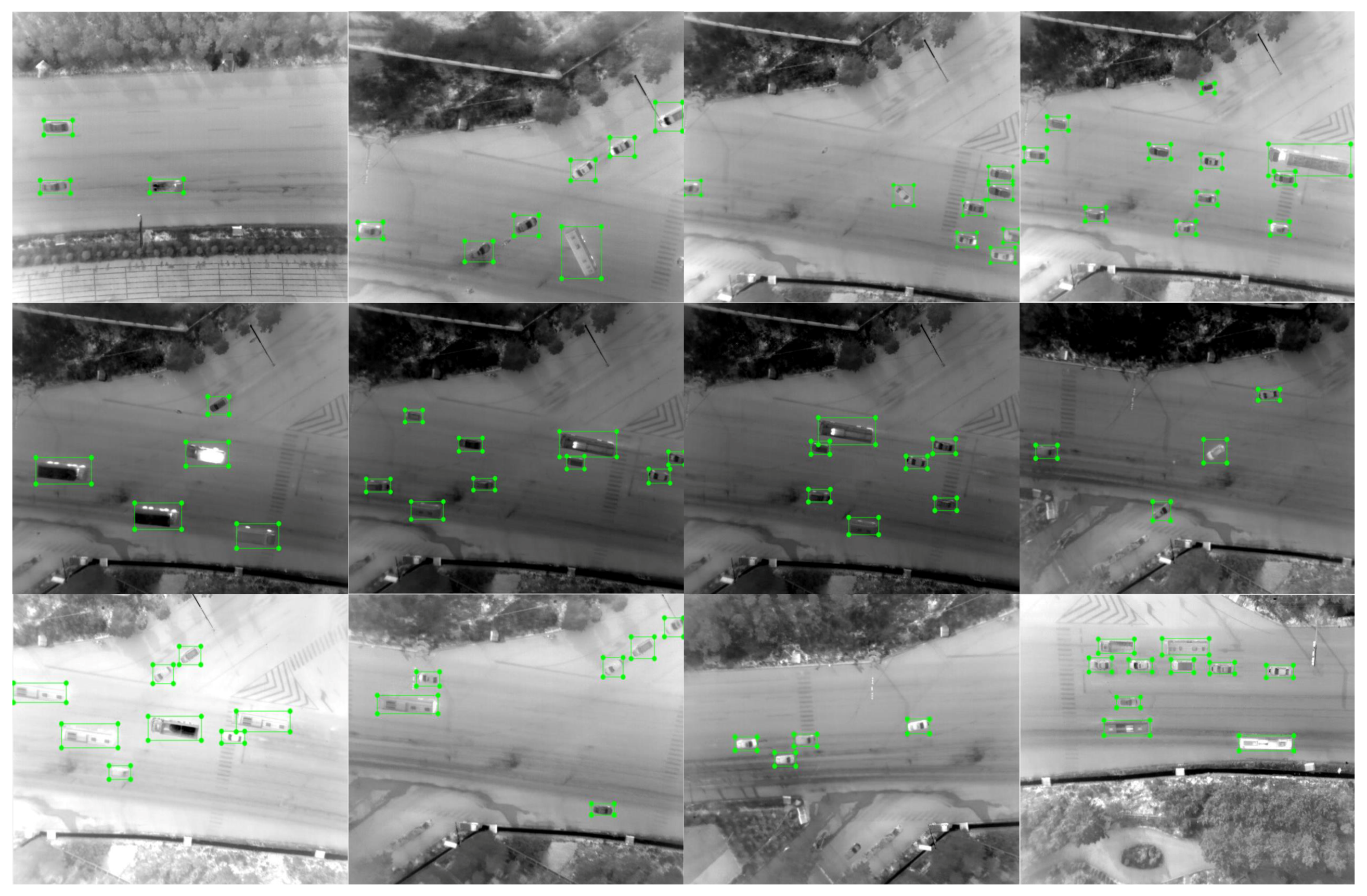
37]. The labeled results are shown in
Figure 3. This labeling step is pivotal to training [
38]. The second step is devoted to sample region feature extraction in a convolutional neural network. We use data augmentations like rotation, crops, exposure shifts and more to expand samples. For training, we adopt a pre-trained classification network on ImageNet [
39], and then fine-tune this. The pre-trained model on the ImageNet has many optimization parameters. On the basis of this, the loss function can be convergent rapidly in the training process. We add a region proposal layer to predict vehicles’ coordinates (
x,
y, width, height) and corresponding confidence. These outputs contain many false alarms and redundant bounding boxes. We remove false alarms by confidence threshold. Finally, non-maximum suppression is adopted to eliminate redundant bounding boxes.
2.1. Label Train Samples
Before labeling, it is necessary to construct an aerial infrared system to capture images for training samples. The aerial infrared system is mainly composed of the DJI Matrice 100 and the FLIR TAU2 camera. The DJI Matrice 100’s major components are made of carbon fiber, which makes it light and solid, in order to guarantee it flies smoothly. The infrared sensor possesses the ability of temperature measurement and various color models’ conversion, which meets the rigorous demands in several environments. In the capture, an intersection filled with a large volume of traffic is chosen as a flight place. Aerial images are captured at five different times alone. Images chosen from the first four times are train samples. Furthermore, aerial infrared vehicle samples from the public data VIVID_pktest are added.
Before training, it is necessary to label large amounts of training samples. These green rectangular regions rectangled in
Figure 3 are some labeled samples. Partial vehicles appear in the image due to the limited view of infrared sensors, especially when it turns a corner, passes through the road or starts to enter into view, so we may catch the front or rear of some vehicles. These pieces of information are helpful because the vehicles often pass through an intersection or make a turn. This information mentioned above can ensure sample integrity. The information captured is crucial for vehicle detection.
In the label process, we obtain some vehicle patches in the infrared images. This guarantees that more training samples are captured and more situations are collected as much as possible. Although this operation is time-consuming and implemented offline, it insures vehicle samples’ integrity [
38]. This can avoid rough sample segmentation. We could observe some part vehicles in the left in 1–3 (row-col) in
Figure 3. This is because the vehicle starts to come into view. There are some moving vehicles close to each other in (3–4) and (2–3). Once roughly segmented, the neighborhoods could be mistaken for just one, but there are two or more vehicles in practice.
All the vehicles are labeled in the training sample, then each image and vehicle position are made into a xml format as the voc [
40].
2.2. Convolutional Neural Network
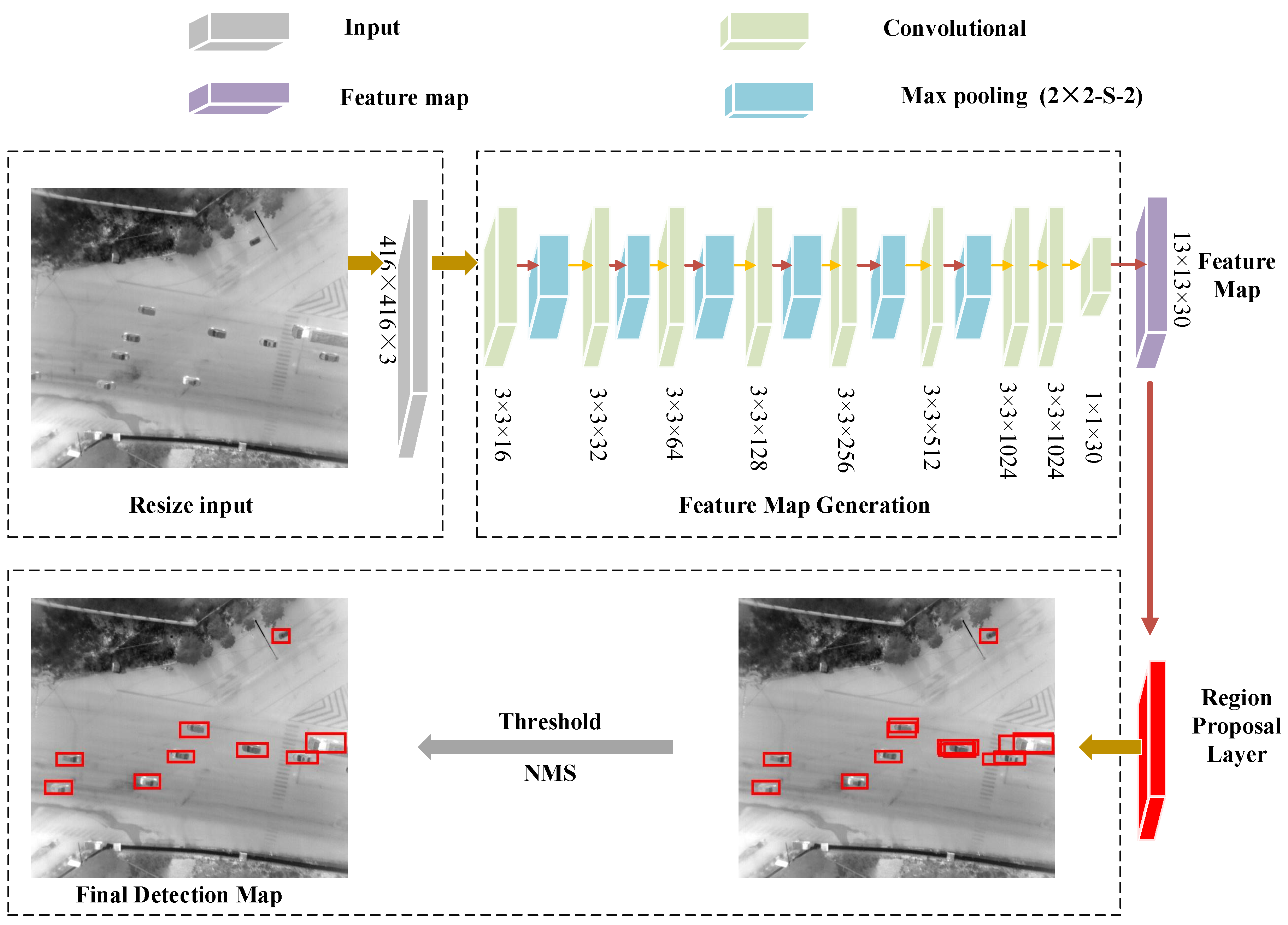
With respect to vehicle detection in aerial infrared images, we apply a convolutional neural network to the full image. It is based on the regressive idea to accomplish the object (vehicles) detection, rather than a typical classification problem. The network designed extracts features and trains on the full images, not the local positive and negative samples. The neural network’s architecture is shown in
Figure 4. Firstly, we resize the input image into 416 × 416, and utilize the convolutional layer and pooling layer by turning to an extract feature. Inspired by the fact that the Faster R-CNN [
31] predicts offset and confidence for bounding boxes using the region proposal, we adopt a region proposal layer to predict bounding boxes. A lot of bounding boxes are obtained this way. We remove some false bounding boxes with low confidence by a threshold filter, and then eliminate redundant boxes using the non maximum suppression.
Feature Map Generation
The detection framework can be mainly divided into two parts:
feature map generation and
candidate bounding boxes generation. The details of feature map are illustrated in
Table 1. The process is composed of 15 layers: nine convolutional layers and six max pooling layers.
Table 1 illustrates the filters channel, size, input and output of each layer. The original image is resized into 416 × 416 as the input. The convolutional layers downsample it by a factor 32, and the output size is 13 × 13. After this, there exists a single center cell in the feature map. The location prediction is based on the center location mechanism.
We carry out 16 filters (3 × 3) convolution operation on the input (416 × 416 × 3), followed by a 2 × 2 with two strides. Subsequently, the number of filers doubles, but the number of strides for pooling layer remains unchanged. Executing the above operations until the number of filters increases to 512, then the channel of stride on pooling layer is set as 1. This disposal wouldn’t change the channel of the input (13 × 13 × 512). Based on this, we add two 3 × 3 convolutional layers with 1024 filters, following a 1 × 1 convolutional layer with 30 filters. Finally, the original image is turned into 13 × 13 × 30.
2.3. Bounding Boxes Generation
After convolutional and pooling operations, the final output is a 13 × 13 × 30 feature map. We add a region proposal layer following the feature map to predict the vehicle’s location. Inspired by the RPN (region proposal network) of Faster-RCNN [
31], we adopt a region proposal layer to service for vehicle border regression. The core purpose of the region proposal layer is to directly generate region proposals by the convolutional neural network. To generate region proposals, we slide a small network over the feature map output by the last shared convolutional layer. The small network takes a 3 × 3 spatial window as input on the feature map. The sliding window is mapped to a 30-dimensional feature vector. The feature is fed into a box-regression layer this way.
At each sliding-window, we simultaneously obtain a great deal of region proposals. Supposing the number of the proposals for each location is R, the output of region proposal layer is coordinates, which are the R boxes’ parametric expressions. The five classes about the proposals’ percentages of width and height are (1.08, 1.09), (3.42, 4.41) , (6.63, 11.38) , (9.42, 5.11), (16.62, 10.52).
2.3.1. Vehicle Prediction on Bounding Boxes
The detection network is an end-to-end neural network. The vehicle’s bounding boxes are accomplished directly by the network, The bounding boxes are achieved in the
bounding boxes generation section. The confidence is computed as Equation (
1):
where
indicates whether there exists a vehicle in the current prediction box, the
is the intersection over union between the predicted box and the ground truth. If no vehicle, the
is 0, 1, otherwise.
The confidence reflects the confidence level if the box contains a vehicle. A new parameter: is added, and each bounding box can be parameterized by .
During the practical evaluating process, these above values are normalized to the range of
. The
reflects the probability of predicted boxes belonging to the vehicle. The
is defined as follows:
2.3.2. Non Maximum Suppression
In order to eliminate redundant bounding boxes, we use non maximum suppression to find the best bounding box for each object. It is used to suppress non-maxima elements and search the local maxima value. The NMS [
41,
42] is for selecting high score detections and skipping windows covered by a previously selected detection.
The left-top corner (
,
), right-bottom corner (
,
), and
of detection boxes are the inputs in the NMS. The (
,
) and (
,
) are calculated by the following equations:
The area of each bounding box is calculated by Equation (
7):
Then, the bounding boxes are sorted by confidence, and the overlap area of box
i and
j is computed by Equation (
12):
Once the is over the suppression threshold, the bounding box with lower confidence would be discarded and the bounding box with highest confidence would be finally kept.
We unconditionally retain the box with higher confidence in each iteration, then calculate the overlap percentage between the box with the highest confidence and the other boxes. If the overlap percentage is bigger than 0.3, the current iteration terminates. The best box is determined until all the regions have been traversed.
3. Aerial Infrared System and Dataset
How we obtain the aerial infrared images (equipments and flight height) and prepare training samples and test images will be demonstrated in this section. In the test, we verify the method on the
VIVID_pktest1 [
36], which has a pretty outstanding performance. However, these images in VIVID_pktest1 can not represent the aerial infrared images in the actual flight.
We capture the actual aerial infrared images (five different times) at an intersection. Experiments are implemented based on the Darknet [
43] framework and run on a graphics mobile workstation with Intel core i7-3770 CPU (Santa Clara, California, US), a Quard K1100M of 2 GB video memory, and 8 GB of memory. The operating system is Ubuntu 14.04 (Canonical company, London, UK).
3.1. Aerial Infrared System
To evaluate the proposed vehicle detection approach, we have constructed an aerial infrared system, which is composed of the DJI Matrice 100 and the FLIR TAU2 camera.
Experiments are conducted by using aerial infrared images with 640 × 512 resolution, which are captured by a camera mounted on a quad rotor with a flight altitude of about 120 m above the ground.
Figure 5 shows the basic components of the system, its referenced parameters are illustrated in
Table 2. The dataset is online at [
35].
3.2. Dataset
3.2.1. Training Samples
VIVID_pktest Sample: As we all know, the VIVID is a public data set for object tracking, which is composed of three subparts. The second part(VIVID_pktest2) [
44] is a training sample. The image sequences are continuous in time, and the adjacent frames are similar to each other. If all images are put into training, the samples are filled with redundancy, so we only choose a set of 151, but which cover all vehicles appearing in VIVID_pktest2.
The authentical infrared sample: For the actual aerial infrared images, an intersection filled with large traffic volume is chosen as a flight place. We capture vehicle samples at five different times alone and choose sample images from the the first four times. The sampling frequency is 10 fps. Finally, we select 368 images, each of which is different in vehicle number, shape and color, as training samples considering redundant samples.
3.2.2. Test Images
As for evaluating the proposed method, we prepare four aerial infrared test image groups. The NPU_DJM100_1, NPU_DJM100_2 and Scenes Change are all captured over Xi’an, China. Four scenes with different backgrounds, flying altitudes, recording times and outside temperatures are used for testing (seen
Table 3).
VIVID_pktest1: The VIVID_pktest1 [
36] is the first test image group, which is used for testing the detection network trained by the sample from the VIVID_pktest2 [
44]. The VIVID_pktest1 is captured at an 80 m high altitude, which contains 100 images and 446 vehicles. The size is 320 × 240.
NPU_DJM100_1: The sample chosen and their adjacent images from the aerial infrared images captured in the first four times is removed, then the remaining is used as the second test image group.
NPU_DJM100_2: The images captured at the fifth time are the third test image group. There are few connections with images belonging to the previous four times.
Scenes Change: The images are captured at earlier times and 80 m flight height. There is not a lot of traffic. This scene is totally different from all of the above. It is used to eliminate scenario training possibilities.
3.3. Training
In training, we use a batch size of 32, a max batch of 5000, a momentum of 0.9 and a decay of 0.0005. Through the training, the learning rate is set as 0.01. In each convolutional layer, we implement a batch normalized disposal except for the final layer before the feature map. With respect to the exquisitely prepared sample images, we divide them at a ratio of 7:3. Seventy percent were used for training, the remaining is for validation.
Loss function: In the objective module, we use the Mean Squared Error (MSE) for training.
where
S is the dimension’s number of the network’s output,
is the error of coordinates between the predicted and the labeled,
is the overlap’s error, and
is the category of error (vehicle or non-vehicle). In the experiment, we amend Equation (
13) by the following:
(1) The coordinates and the IOU (intersection over union) have different contribution degrees to the Loss, so we set the to amend the .
(2) For the IOU’s error, the gridding includes the vehicle and the gridding having no vehicle should make various contributions to . We use the to amend the .
(3) As for the equal error, these large objects’ impacts should be lower than small ones on vehicle detection because the percentage of error belonging to large objects is far less than those belonging to small ones. We square the
to improve it. The final Loss is as Equation (
14):
where the
x,
y,
w,
h,
C,
p are the predicted, and the
,
,
,
,
,
are the labeled. The
and the
reflect that the probability of that object is in, and not in, the
j bounding boxes, respectively.
5. Conclusions
This paper proposes an efficient method for real-time ground vehicle detection in infrared imagery based on a convolutional neural network. In the proposed approach, we exploit a convolutional neural network to mine the abundant abstract features among the aerial infrared imagery. These features are more distinguished in ground vehicle detection. For ground vehicle detection, we firstly build a real-time ground vehicle detection system to capture real scene aerial images. All of the manually labeled training samples and test images are publicly posted. Then, we construct the convolutional and pooling layers and region proposal layer to achieve feature extraction. The convolutional and pooling layers are adopted to explore the vehicle’s inherent features, and the rear region proposal layer is exploited to generate candidate vehicle boxes. Finally, on the basis of a labeled sample’s feature, the method iteratively learns and memorizes these features to generate a real-time ground vehicle model. It has the unique ability to detect both the stationary vehicles and moving vehicles in real urban environments. Experiments on the four different scenes demonstrate that the proposed method is effective and efficient to recognize the ground vehicles. In addition, it can accomplish the task in real time while achieving superior performances in leak and false alarm ratio. Furthermore, the current work shows great potential for ground vehicle detection in aerial imagery.
In the real world, the real-time ground vehicle detection can be applied to intelligent surveillance, traffic safety, wildlife conservation and so on. In the intelligent surveillance, the system can rapidly give the vehicle’s location in imagery under day and night, which is helpful for traffic monitoring and traffic flow statistics. Traffic crashes might occur in our daily lives all the time, but it is difficult to confirm the responsibility for the accident in complex backgrounds. The system can be used to identify the principal responsible party for its real-time detection capacity. As for the wildlife conservation, most of the protected animals are caught and killed during the night. The system can locate the hunter’s vehicle at night, and this helps some regulatory agencies to take countermeasures in time.


