This section discusses the LiDAR’s beacon detection system.
3.6.1. Overview
The LiDAR data we collect are in the form of a three-dimensional (3D) and 360 degree field-of-view (FOV) point cloud, which consists of
x,
y,
z coordinates, along with intensity and beam number (sometimes called ring number). The coordinates
x,
y and
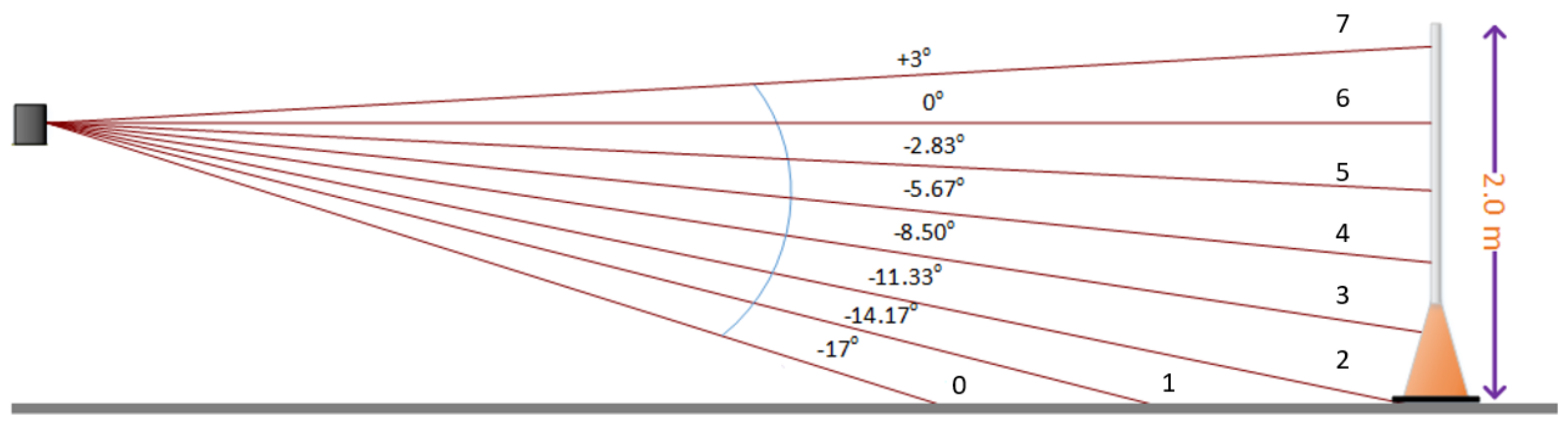
z represent the position of each point relative to the origin centered within the LiDAR. Intensity represents the strength of returns and is an integer for this model of LiDAR. Highly reflective objects such as metal or retro-reflective tape will have higher intensity values. The beam number represents in which beam the returned point is located. The LiDAR we use transmits eight beams. The beam numbers are shown in
Figure 9. Assuming the LiDAR is mounted level to the ground, then Beam 7 is the top beam and is aimed upward approximately 3°. Beam 6 points horizontally. The beams are spaced approximately 3° apart.
Figure 10 shows one scan of the LiDAR point cloud. In this figure, the ground points are shown with black points. The beacon presents as a series of closely-spaced points in the horizontal direction, as shown in the square.
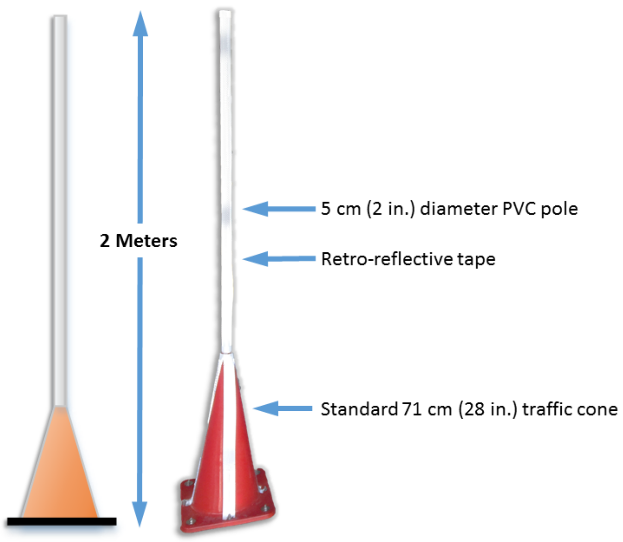
General object detection in LiDAR is a difficult and unsolved problem in the computer vision community. Objects appear at different scales based on their distance to the LiDAR, and they can be viewed from any angle. However, in our case, we are really only interested in detecting the beacons, which all have the same geometries. In our application, the industrial vehicle can only go so fast, so that we only need to detect beacons about 20 m away or closer. The beacons are designed to have very bright returns. However, other objects can also have bright returns in the scene, such as people wearing safety vests with retro-reflective tape, or other industrial vehicles. Herein, we propose a system that first identifies clusters of points in the scene that present with bright returns. Next, a linear SVM classifier is used to differentiate the beacon clusters from non-beacon clusters.
The LiDAR detection system works by utilizing intensity-based and density-based clustering (a modified DBSCAN algorithm) on the LiDAR point cloud. The system then examines all points near the cluster centroid by extracting features and using a linear SVM to discriminate beacons from non-beacons. Details of these algorithm are discussed in the subsections below.
3.6.3. LiDAR Feature Extraction
To extract the features, the ground points must be removed before feature processing occurs, or else false alarms can occur. Since this industrial application has a smooth, flat area for the ground, we employ a simple vertical threshold to remove ground points. If this system were to be generalized to areas with more varying ground conditions, ground estimation methods such as those in [
42,
43,
44,
45,
46,
47] could be utilized. However, for this particular application, this was not necessary.
Next, the point intensities are compared to an empirically-determined threshold. The beacon is designed so that it provides bright returns to the LiDAR via the retro-reflective vertical pole. This works well, but there are also other objects in the scene that can have high returns, such as other industrial vehicles with retro-reflective markings or workers wearing safety vests with retro-reflective stripes. In order to classify objects as beacons and non-beacons, hand-crafted features are utilized (these are discussed below). After ground-removal and thresholding the intensity points, we are left with a set of bright points. A second set of intensity points is also analyzed, which consists of all of the non-ground points (e.g., the point cloud after ground removal). The points in the bright point cloud are clustered. Beacons appear as tall, thin objects, whereas all other objects are either not as tall, or wider. We extract features around the cluster center in a small rectangular volume centered at each object’s centroid. We also extract features using a larger rectangular volume also centered around the objects centroid. Features include counting the number of bright points in each region, determining the x, y and z extents of the points in each region, etc. Beacons mainly have larger values in the smaller region, while other objects have values in the larger regions.
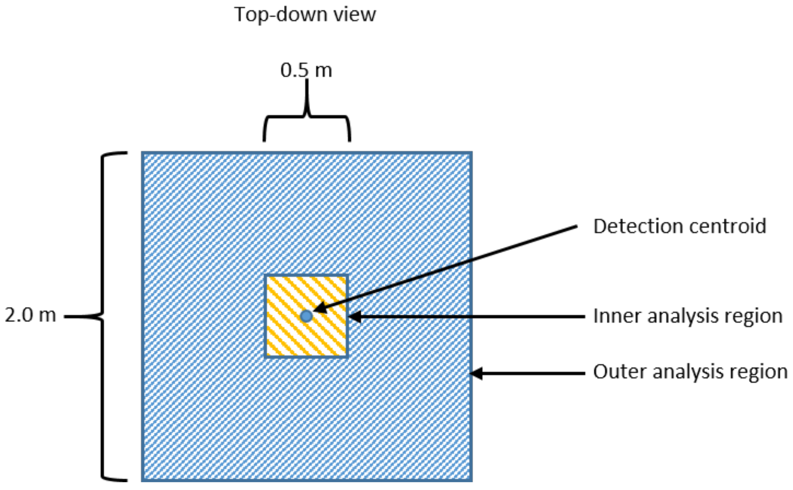
The two regions are shown in
Figure 11. The idea of using an inner and an outer analysis region is that a beacon will mostly have bright points located in the inner analysis region, while other objects, such as humans, other industrial vehicles, etc., will extend into the outer regions. Equations (
1) and (
2) define whether a LiDAR point
with coordinates
is in the inner region or outer region, respectively, where the object’s centroid has coordinates
. Reference
Figure 11 for a top-down illustration of the inner and outer regions.
Figure 11 shows an example beacon return with the analysis windows superimposed. Both the inner and outer analysis regions have
x and
y coordinates centered at the centroid location. The inner analysis region has a depth (
x coordinate) of 0.5 m and a width (
y coordinate) of 0.5 m, and the height includes all points with
z coordinate values of −1.18 m and above. The outer region extends 2.0 m in both
x and
y directions and has the same height restriction as the inner region. These values were determined based on the dimensions of the beacon and based on the LiDAR height. The parameters
,
and
define the inner region relative to the centroid coordinates. Similarly, the parameters
,
and
define the outer region relative to the centroid coordinates. A point is in the inner region if:
and a point is in the outer region if:
In order to be robust, we also extract features on the intensity returns. A linear SVM was trained on a large number of beacon and non-beacon objects, and each feature was sorted based on its ability to distinguish beacons from non-beacons. In general, there is a marked increase in performance, then the curve levels out. It was found that ten features were required to achieve very high detection rates and low false alarms. These ten features were utilized in real time, and the system operates in real time at the frame rate of the LiDAR, 5 Hz. The system was validated by first running on another large test set independent of the training set, with excellent performance as a result as presented in
Section 3.6.4. Then, extensive field tests were used to further validate the results as presented in
Section 4.
After detection, objects are then classified as beacons or non-beacons. These are appended to two separate lists and reported by their distance in meters from the front of the industrial vehicle, their azimuth angle in degrees and their discriminate value. Through extensive experimentation, we can reliably see beacons in the LiDAR’s FOV from 3 to 20 m.
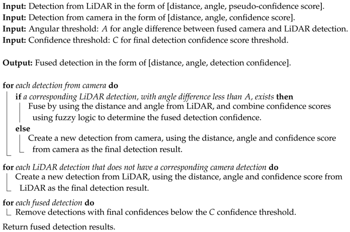
LiDAR feature extraction follows the overall algorithm shown in Algorithm 2. The input is the LiDAR point cloud , where j is the index variable for the j-th point, and x, y, z, i and r refer to the x point in meters, the y point in meters, the z point in meters, the intensity and the beam number, respectively, for the j-th point. Note that all coordinates are relative to the center of the LiDAR at point . The x coordinate is positive in front of the LiDAR, and negative behind. The y coordinate is positive to the left of the LiDAR and negative to the right. The z coordinate is positive above the LiDAR and negative below.
| Algorithm 2: LiDAR high-level feature extraction preprocessing. |
![Electronics 07 00084 i002]() |
In order to extract features for objects, any points that did not provide a return to the LiDAR are removed. These points will present as NaN’s (not a number) in the LiDAR point cloud. Next, the estimated ground points are removed. The non-ground points are divided into two data subsets: The high-threshold (HT) data and the low-threshold (LT) data. The HT data points only contain high-intensity returns, while the LT data contain points greater than or equal to the low-intensity threshold. Both data subsets do not contain any ground points. The high-intensity threshold was set to 15 and the low-intensity threshold to zero. These threshold values were determined experimentally based on the examination of multiple beacon returns at various distances.
| Algorithm 3: LiDAR feature extraction. |
![Electronics 07 00084 i003]() |
Table 1 describes the extracted features. For example, Feature 1 is generated from the high threshold data, which consists solely of high-intensity points. The data is analyzed only for high-intensity points in the inner analysis region. This feature simply computes the
Z (height) extent, that is, the maximum
Z value minus the minimum
Z value. Note that some of the features are only processed on certain beams, such as Feature 2. The features are listed in order of their discriminate power in descending order, e.g., Feature 1 is the most discriminate, Feature 2 the next most discriminate, etc. Initially, it was unknown how effective the features would be. We started with 134 features, and these were ranked in order of their discriminating power using the score defined as:
where
,
,
and
are the number of true positives, true negatives, false positive and false negatives, respectively [
48]. A higher score is better, and scores range from zero to 1000. This score was used since training with overall accuracy tended to highly favor one class and provided poor generalizability, which may be a peculiarity of the chosen features and the training set.
Figure 12 shows the score values versus the number of features (where the features are sorted in descending score order. The operating point is shown for
features (circles in the plot). The features generalize fairly well since the testing curve is similar to the training curve. In our system, using 20 features provided a good balance of performance versus computational complexity to compute the features. Each LiDAR scan (5-Hz scan rate) requires calculating features for each cluster. Experimentation showed that a total of 20 features was near the upper limit of what the processor could calculate and not degrade the LiDAR processing frame rate.
3.6.4. SVM LiDAR Beacon Detection
To detect the beacons in the 3D LiDAR point cloud, we use a linear SVM [
49], which makes a decision based on a learned linear discriminant rule operating on the hand-crafted features we have developed for differentiating beacons. Herein, liblinear was used to train the SVM [
50]. A linear SVM operates by finding the optimal linear combination of features that best separates the training data. If the
M testing features for a testing instance are given by
, where the superscript
T is a vector transpose operator, then the SVM evaluates the discriminant:
where
is the SVM weight vector and
b is the SVM bias term. Herein,
M was chosen to be 20. Equation (
4) applies a linear weight to each feature and adds a bias term. The discriminant is optimized during SVM training. The SVM optimizes the individual weights in the weight vector to maximize the margin and provide the best overall discriminant capability of the SVM. The bias term lets the optimal separating hyperplane drift from the origin.
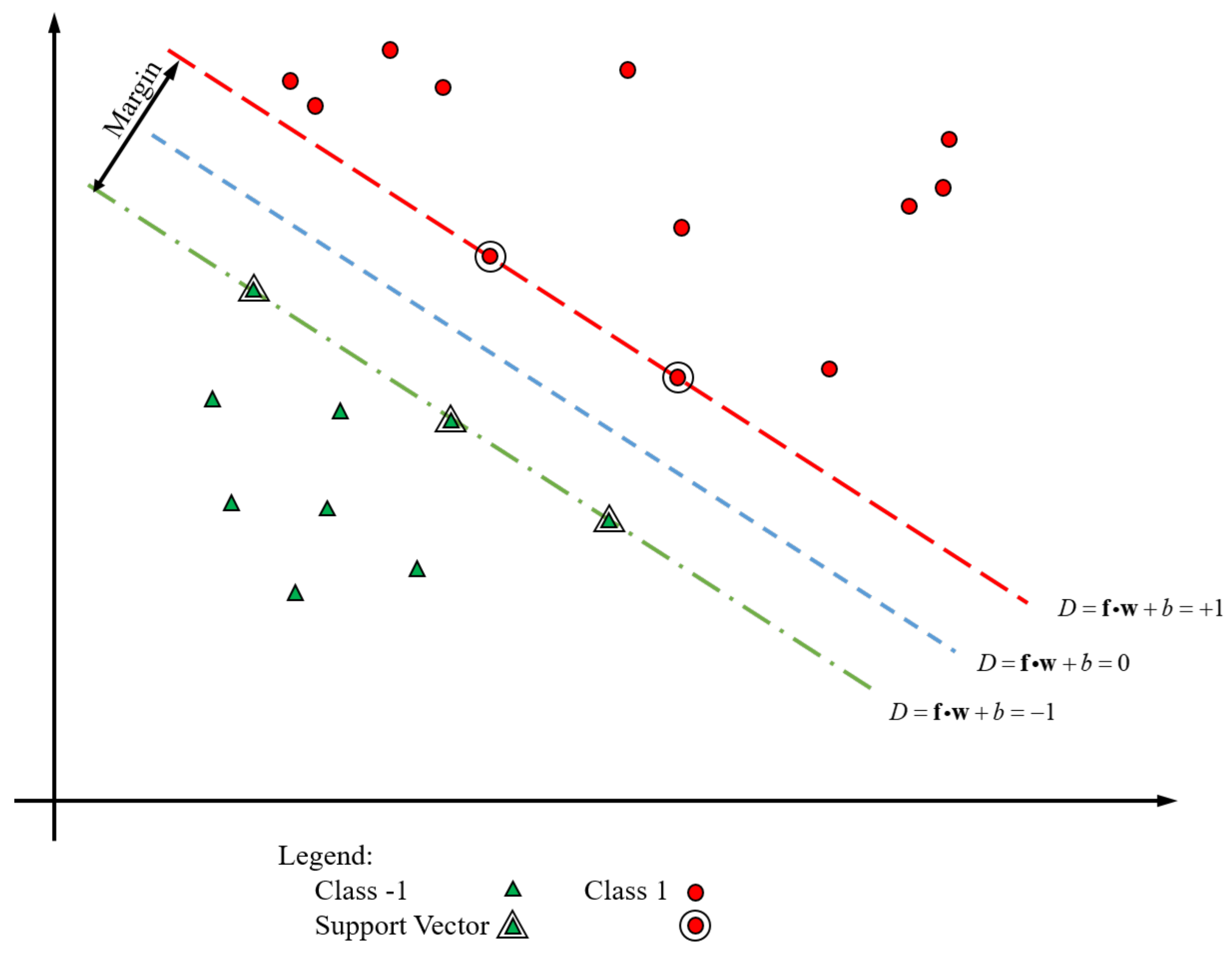
Figure 13 shows an example case with two features. In this case, the
hyperplane is the decision boundary. The
and
hyperplanes are determined by the support vectors. The SVM only uses the support vectors to define the optimal boundary.
The SVM was trained with beacon and non-beacon data extracted over multiple data collections. There were 13,190 beacon training instances and 15,209 non-beacon training instances. The test data had 12,084 beacons and 5666 non-beacon instances.
In this work,
features were chosen. Each feature is first normalized by subtracting the mean of the feature values from the training data and dividing each feature by four times the standard deviation plus
(in order to prevent division by very small numbers). Subtracting the mean value centers the feature probability distribution function (PDF) around zero. Dividing by four times, the standard deviation maps almost all feature values into the range
, because most of the values lie within
. The normalized features are calculated using:
where
is the mean value of feature
k and
is the standard deviation of feature
k for
. The mean and standard deviation are estimated from the training data and then applied to the test data. The final discriminant is computed using Equation (
4) where the feature vector is the normalized feature vector.
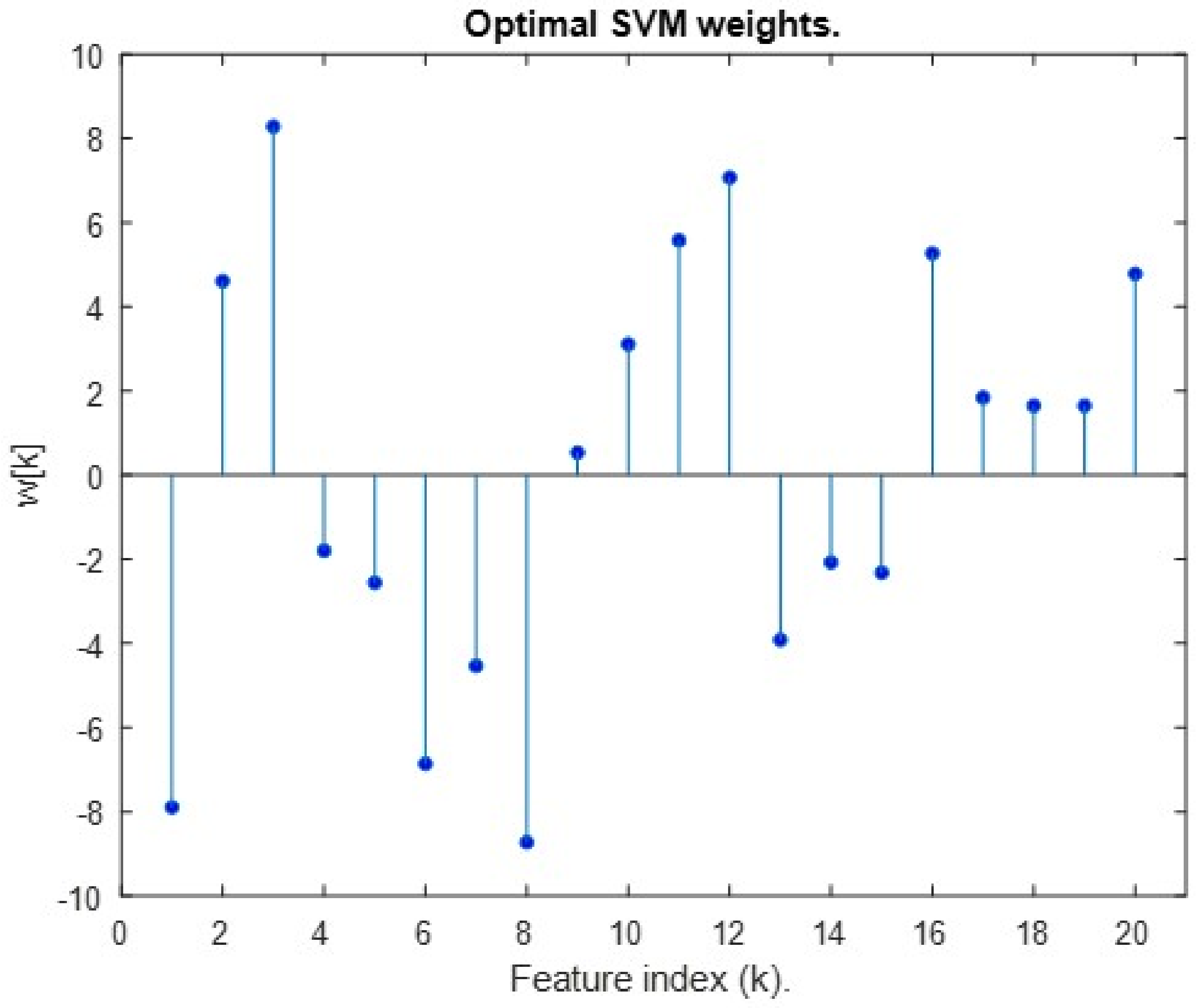
The optimal feature weighs are shown in
Figure 14. Since all the features are normalized, Features 1, 3 and 8 have the most influence on the final discriminant function.
If the discriminant
, then the object is declared a beacon. Otherwise, it is declared a non-beacon (and ignored by the LiDAR beacon detection system). Once the SVM is trained, implementing the discriminant given in Equation (
4) is trivial and uses minimal processing time.
Figure 15 shows the PDF of the LiDAR discriminant values for beacons and non-beacons, respectively. The PDFs are nearly linearly separable. The more negative the discriminant values, the more the object is beacon-like.


