To find the relationship between the radiation patterns of elements and the adaptive array performance, the output adaptive array gain in the presence of a desired signal and J interfering signals is studied. It should be pointed out that the impacts of the RF front-end are neglected, and we assume that all the signals are continuous waves.
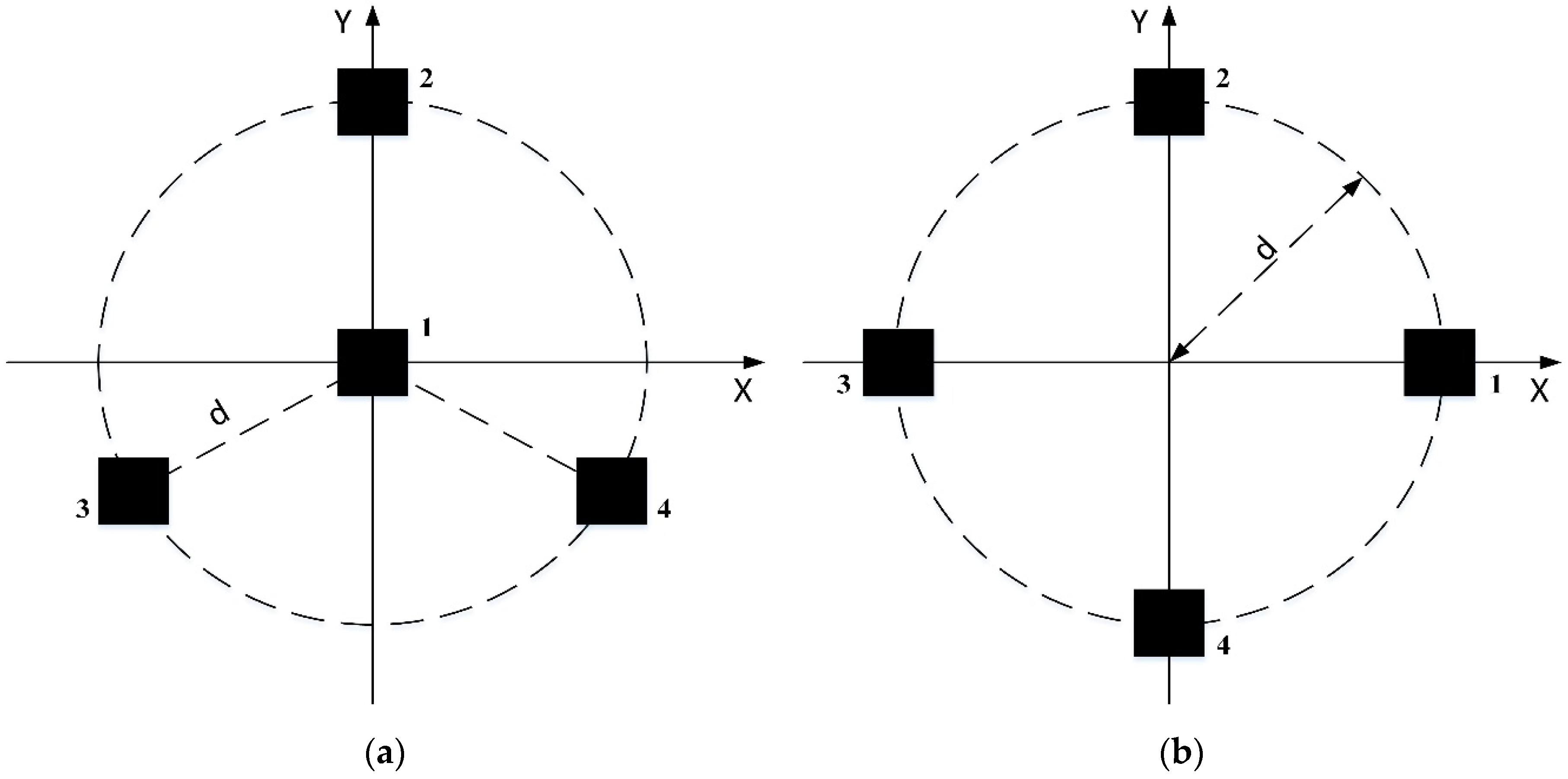
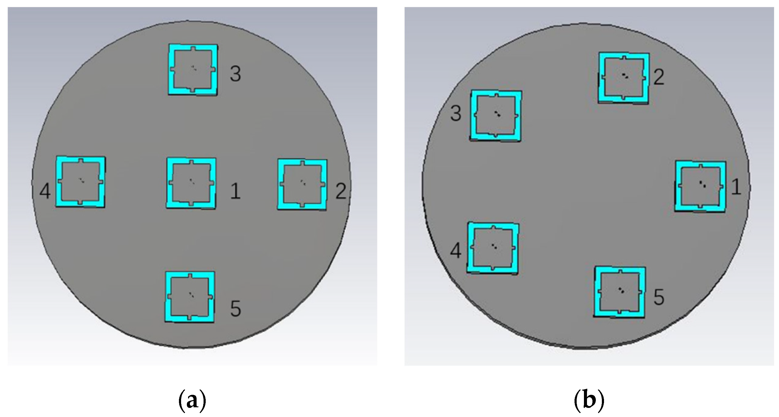
Two different distributions of antenna elements, as shown in
Figure 1, are considered in this paper, which are commonly used as the array geometry for GNSS antenna arrays. Note that the element distribution G1 consisted of elements that are equally spaced on a circle with a half-wavelength radius (i.e., d = 0.5
as shown in
Figure 1) and an element at the circle’s center. In element distribution G2, the antenna elements are uniformly spread on the perimeter of a circle with a radius of half a wavelength.
The square patch element is located on a substrate with a height of 5 mm and a relative dielectric constant of 30. The patch element performs right-hand circular polarization (RHCP) by a dual-feed configuration providing two ports with a 90-degree phase difference. All the patch elements work at 1268.52 MHz, which is the central frequency of the B3 signal of the BeiDou Satellite Navigation System [
21], and their S
11 < −15 dB. We used CST Microwave Studio (Dassault Systems, Vélizy-Villacoublay, France) to simulate the in-situ response of elements in arrays, which is used to investigate the performance of the adaptive arrays through 100 Monte Carlo simulations in MATLAB (Mathworks, Natick, MA, USA). As shown in
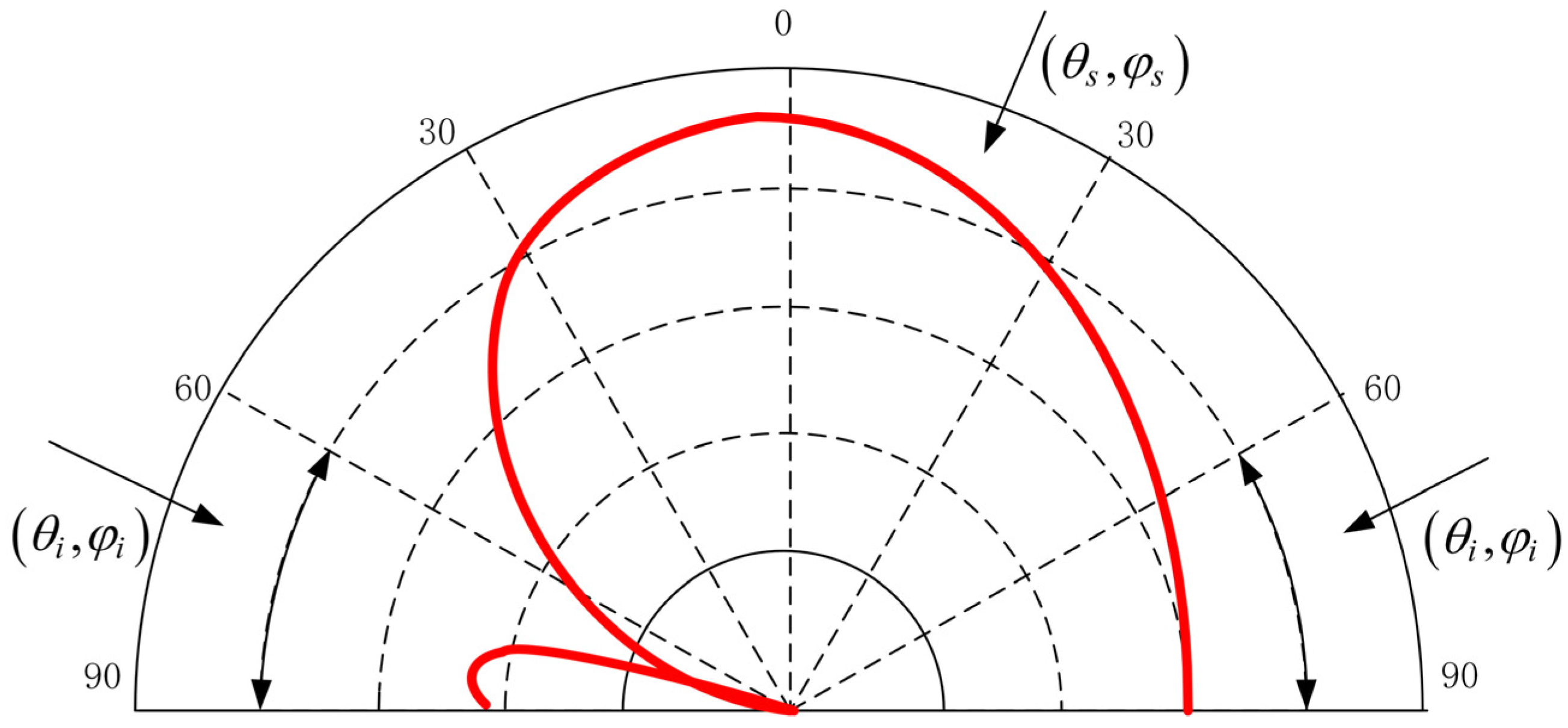
Figure 2, the incident angles of the interfering signals in each simulation are randomized uniformly from the region below 30° elevation, which is the common scenario in practice, while the incident angles of the GNSS signal vary in one-degree steps throughout the entire upper hemisphere. The average availabilities are finally calculated over 100 independent trials. For all simulations, it is assumed that the GNSS signal is 20 dB below the noise floor, and the interference signals are 40 dB above the noise.
3.1. Gain Patterns
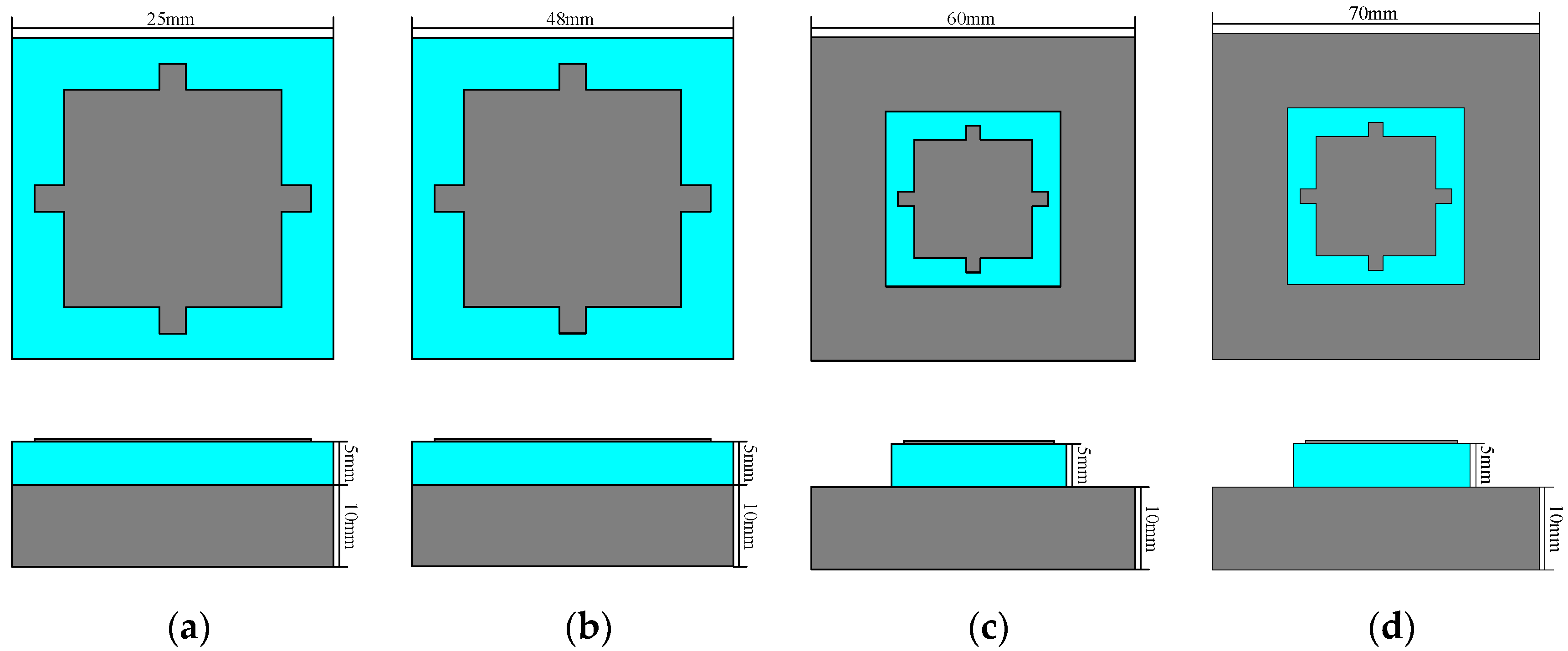
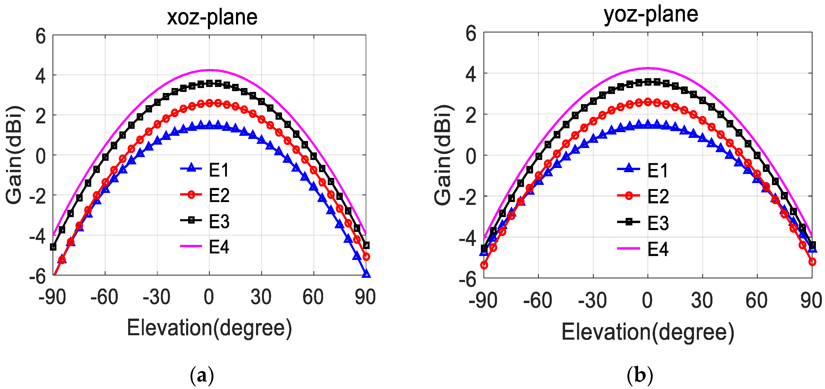
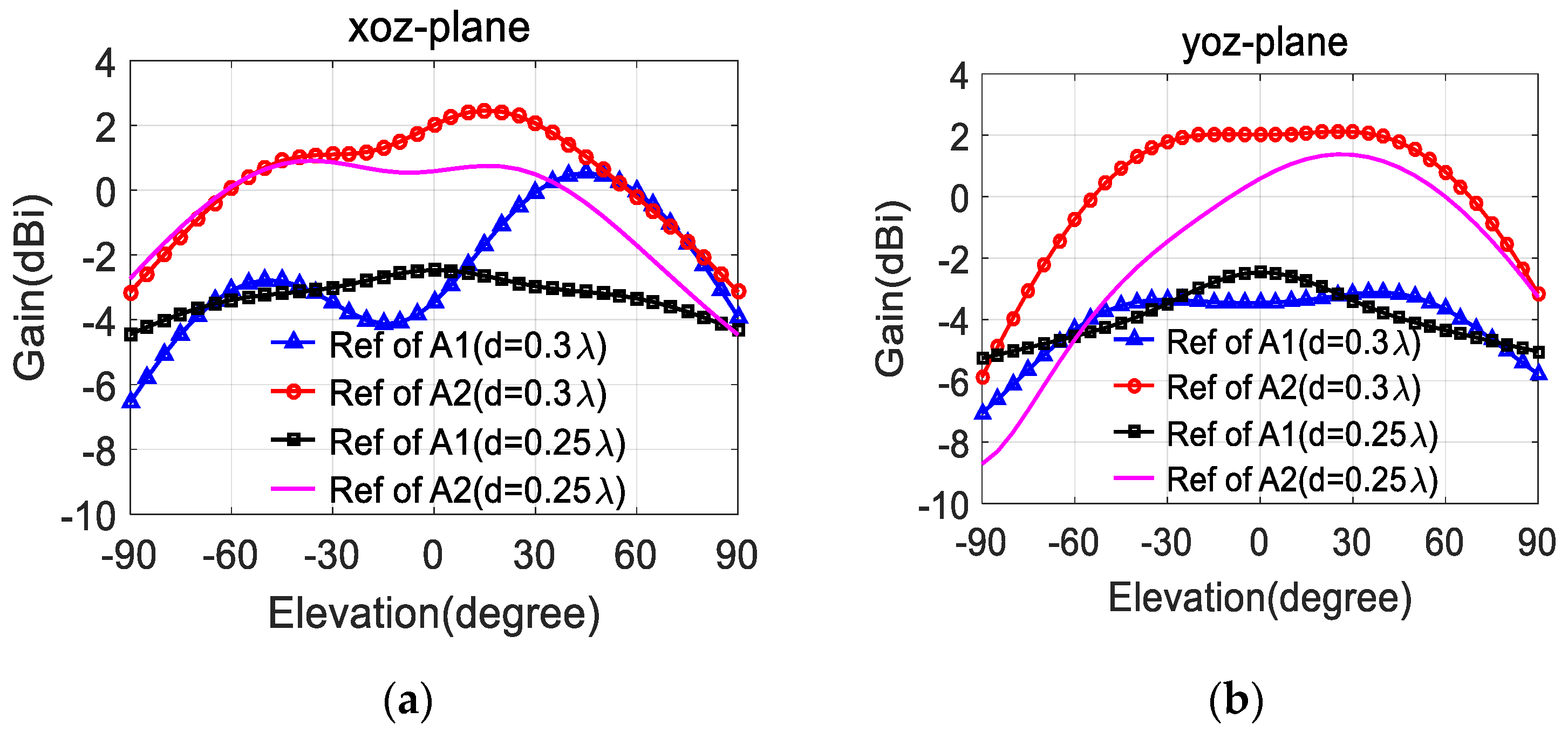
Firstly, the performance of the arrays with different gain patterns of elements is studied, and the effects of phase patterns are neglected here. By changing the size of the antenna aperture, we designed four different antenna elements, named E1, E2, E3 and E4, in CST Microwave Studio (Dassault Systems, Vélizy-Villacoublay, France) (see
Figure 3), and the radiation patterns of these are shown in
Figure 4. These four elements are selected as the reference elements of G1 and G2, respectively. Note that the reference elements are both located at element 1 as shown in
Figure 1 and the other elements are equal.
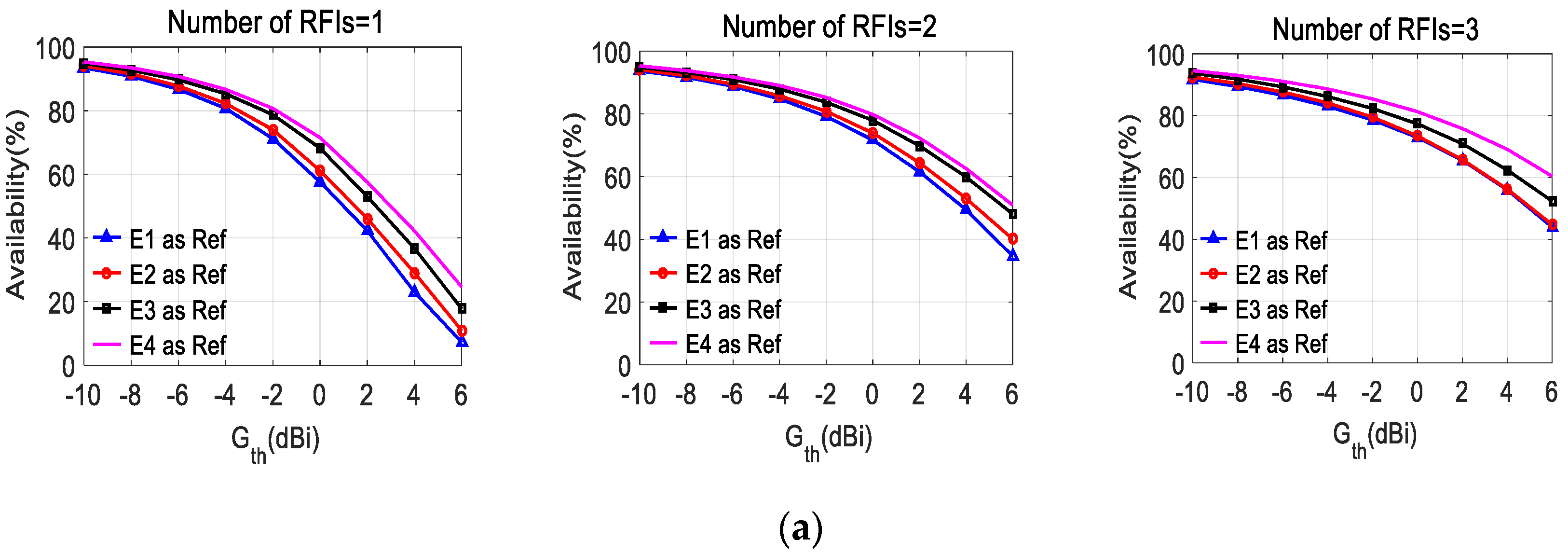
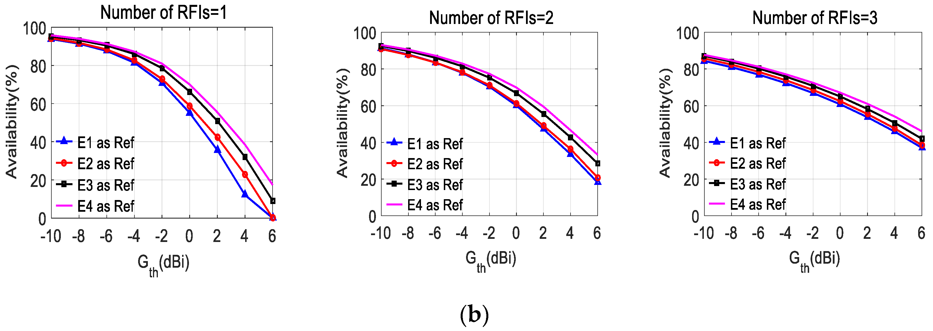
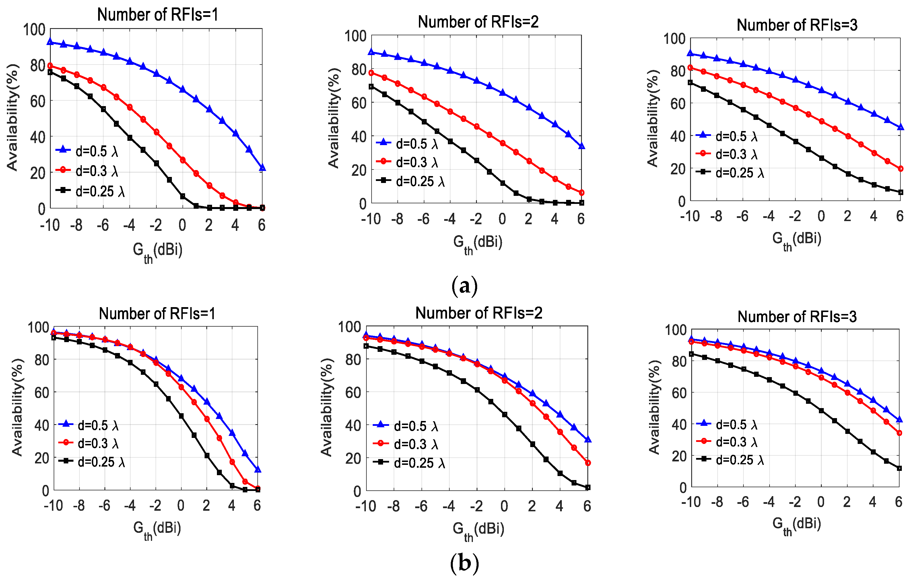
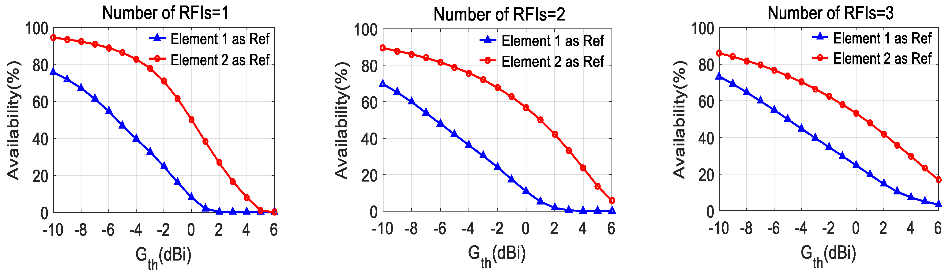
In
Figure 5, the average angular availabilities of arrays with different gain patterns of reference elements are shown as a function of the values of the selected threshold G
th, for the case of G1 and G2, respectively. The results are shown for different numbers of RFIs (radio frequency interferences) in each case. It can be seen from
Figure 5 that the availability improves with the increase of the gain of reference elements under the selected array geometries.
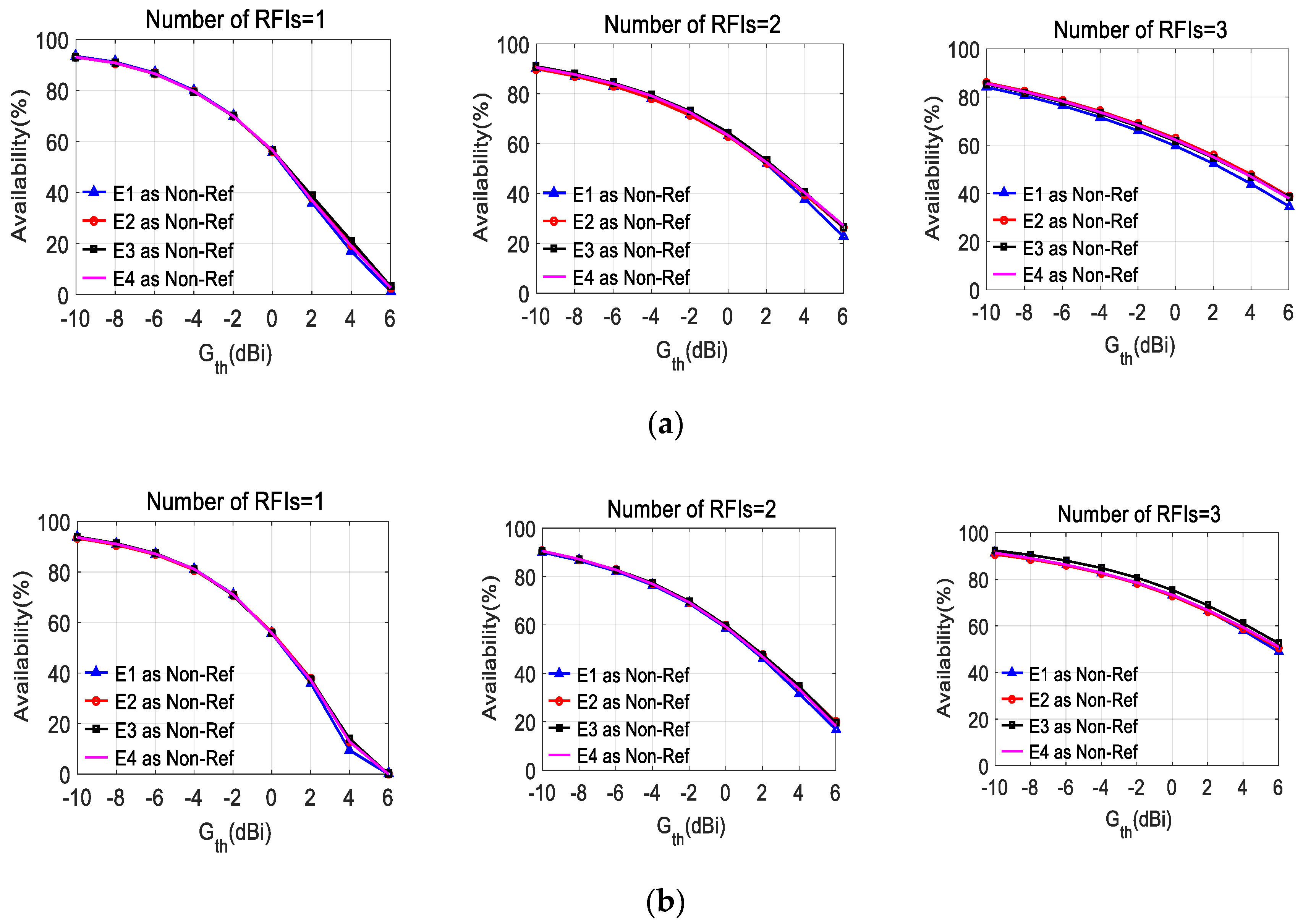
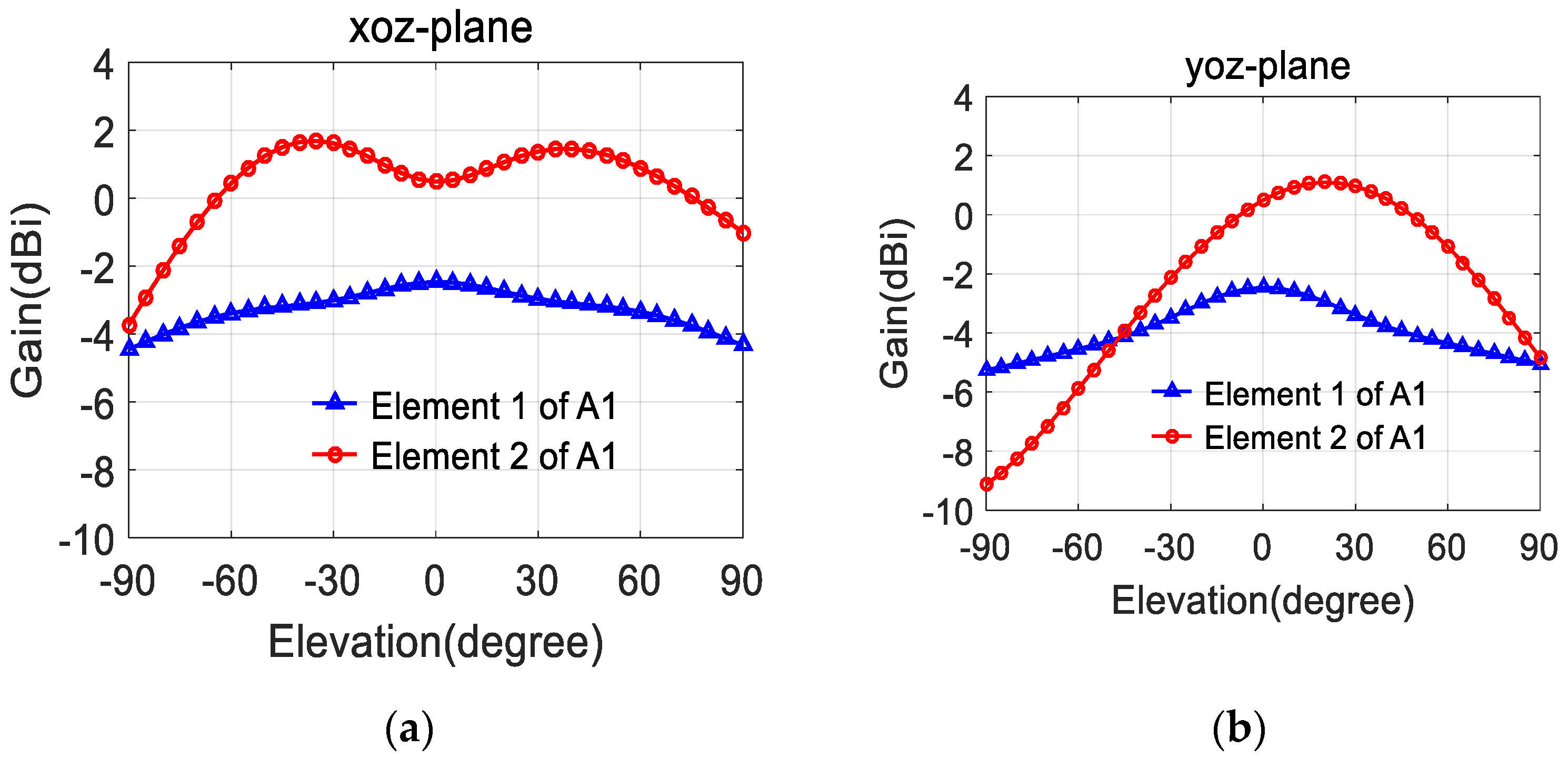
Next, we consider the impact of the extent of the change of non-reference element patterns as compared with the reference pattern on the array performance.
We selected the four elements in
Figure 3 as non-reference elements of G1 and G2, respectively. Note that, in each case, the non-reference elements are identical (E1 or E2 or E3 or E4), and the gain patterns of these are shown in
Figure 4. All reference elements are selected as E1 in different cases and are still located at element 1 as shown in
Figure 1.
Figure 6 plots the performance of the antenna arrays with different gain patterns of non-reference elements. With the non-reference elements selected from E1 to E4, the gain patterns of the non-reference elements vary increasingly compared with those of the reference element, but the availabilities of the array remain nearly the same. It can be concluded that the extent of non-reference element gain pattern changes as compared with the reference pattern has little effect on the availability performance of the array.
Furthermore, it can be seen clearly from the comparison of
Figure 5 and
Figure 6 that the adaptive array gain of the PI array is mainly determined by the radiation pattern of the reference element, while the gain patterns of non-reference elements have little effect on the availability performance of the adaptive array. The good agreement between the results and the theoretical derivation in
Section 2 evidently illustrates that the PI algorithm essentially forces the elements to be in an unequal position This leads to the domination of the radiation characteristics of the reference element on the adaptive array gain.
It should be pointed out that the larger the number of RFIs is, the smaller the effect of the gain of the reference element on the adaptive array gain. As depicted in
Figure 5, the availability performance of the array is mainly dependent on the array factor when the number of interferences is equal to three. Overall, the adaptive array gain of G1 is slightly better than that of G2, as plotted in
Figure 5 and
Figure 6.
3.2. Phase Patterns
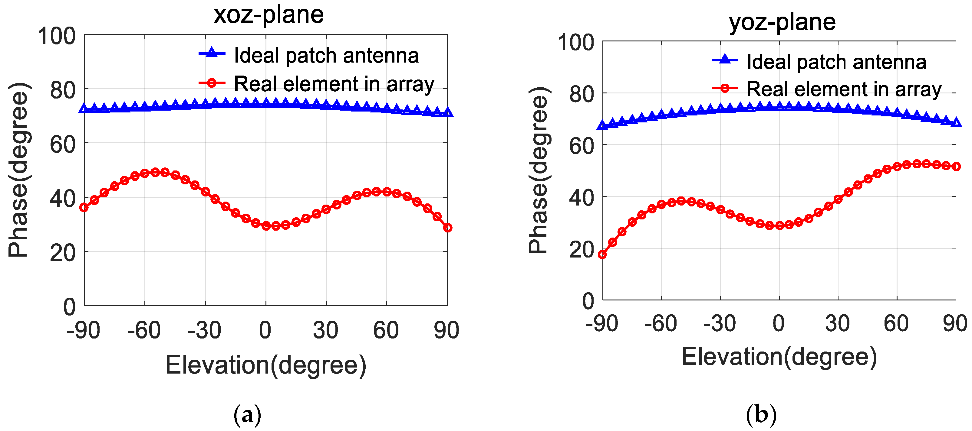
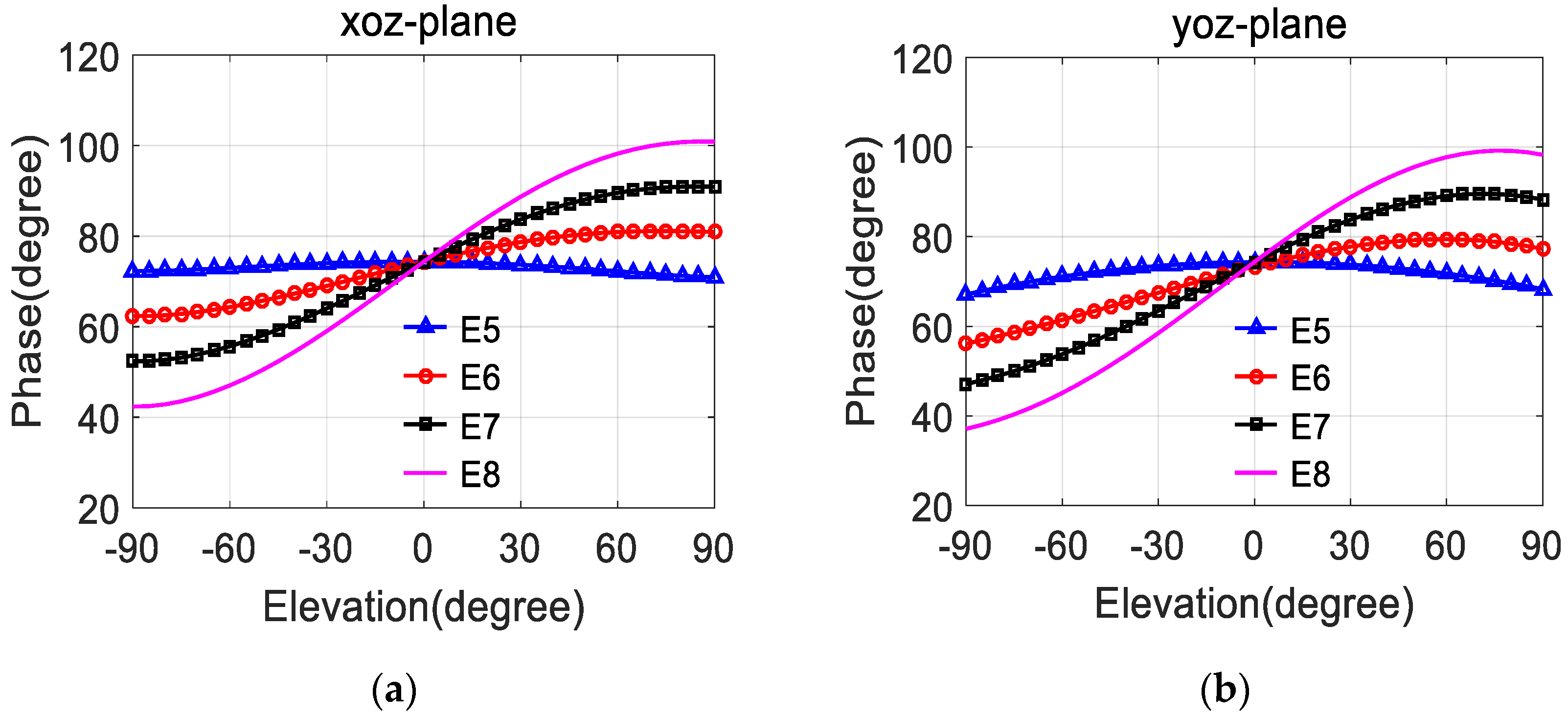
Secondly, the performance of arrays with different phase patterns of antenna elements is investigated. The effect of gain patterns is neglected here. Since the phase is a relative concept, we usually take the zenith direction as the zero-phase reference point. Additionally, the phase pattern of the patch antenna in this paper has some characteristics that are nearly unchanged with the increase of elevation angle; however, the phase will fluctuate with the increase of elevation angle as the patch antenna is located in the array. The phase pattern comparison between the ideal patch antenna and the real element in array is depicted in
Figure 7. Note that the phase fluctuation of the real antenna in the array with the increase of elevation angle is generally from 0 to 30 degrees compared to the zero-phase reference point. According to this characteristic, we artificially designed four different antennas, named E5, E6, E7 and E8, the phase patterns of which are shown in
Figure 8.
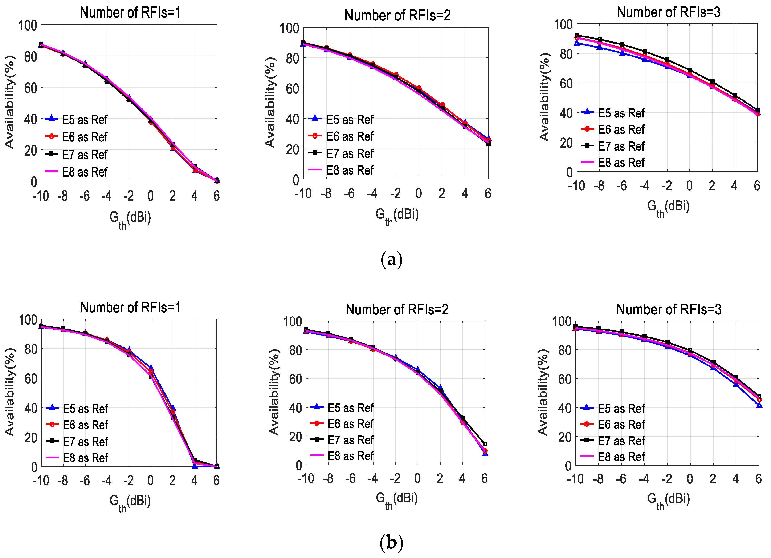
We selected these four elements as the reference elements of G1 and G2, respectively. Note that the reference elements are both located at element 1, as shown in
Figure 1, and the other elements are equal. In
Figure 9, the average angular availabilities of arrays with different phase patterns of reference elements are presented for the case of G1 and G2, respectively. The results are shown for different numbers of RFIs in each case.
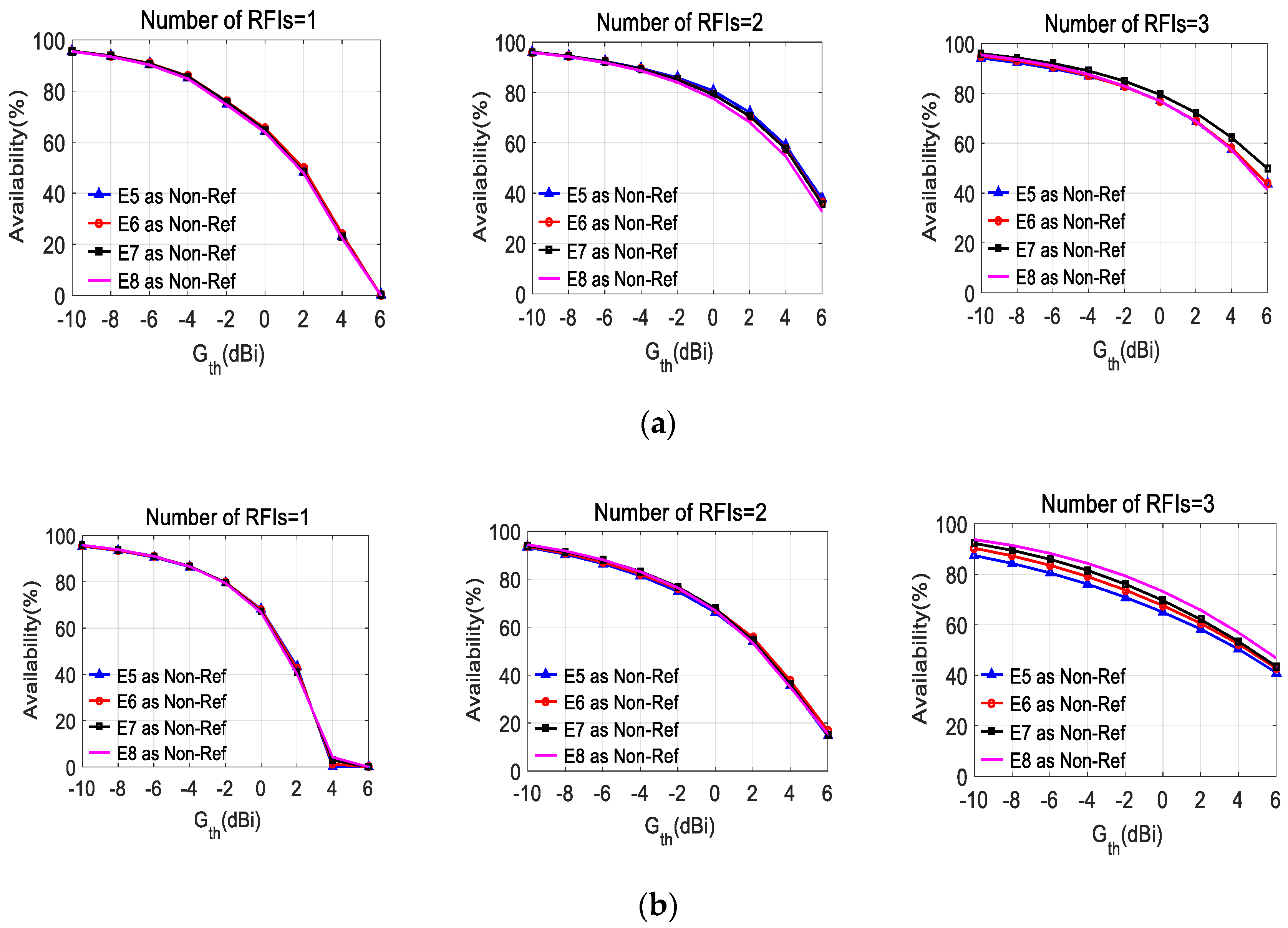
Similarly, these four elements are selected as the non-reference elements of G1 and G2, respectively.
Figure 10 plots the performance of the antenna arrays with different phase patterns of non-reference elements, which are selected from
Figure 8. Note that in different cases, the non-reference elements are identical (E5 or E6 or E7 or E8); the phase patterns are shown in
Figure 8. Furthermore, all reference elements are selected as E5 and are still located at element 1, as shown in
Figure 1.
Obviously, both the phase pattern of the reference element and the non-reference elements have little effect on the availability performance of the PI adaptive array. The results in
Figure 9 and
Figure 10 illustrate that the PI algorithm has a certain adaptability to the phase perturbation of the elements.
Conventionally, as the number of RFIs increases, the availability will degrade since more nulls should be steered towards interferer sources. However, the availabilities in
Figure 5,
Figure 6,
Figure 9 and
Figure 10 increase as the number of RFIs increases. To explain this phenomenon, we choose three specific scenarios in which the numbers of RFIs are one, two, and three, respectively: (a)
; (b)
and
; (c)
,
and
.
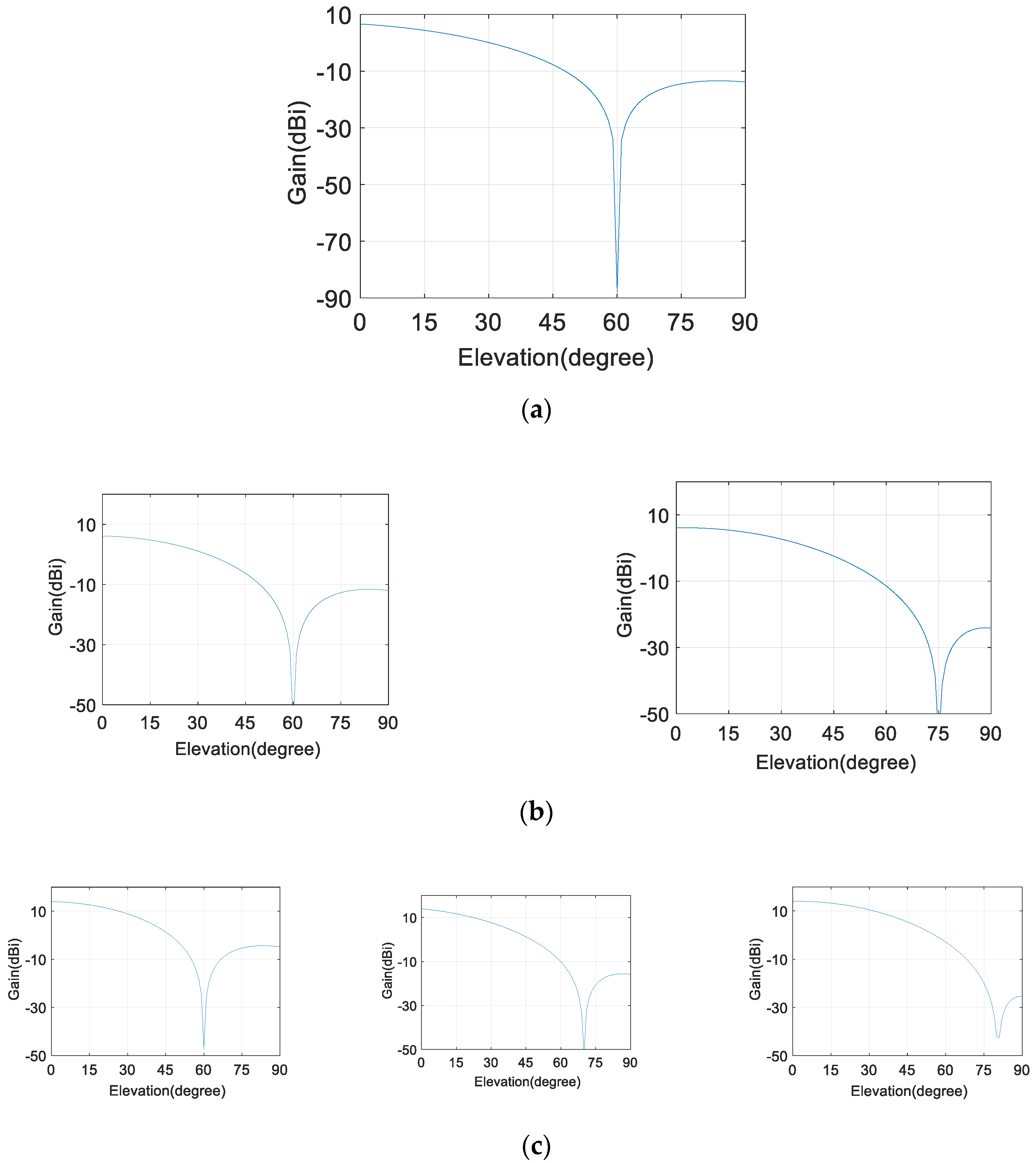
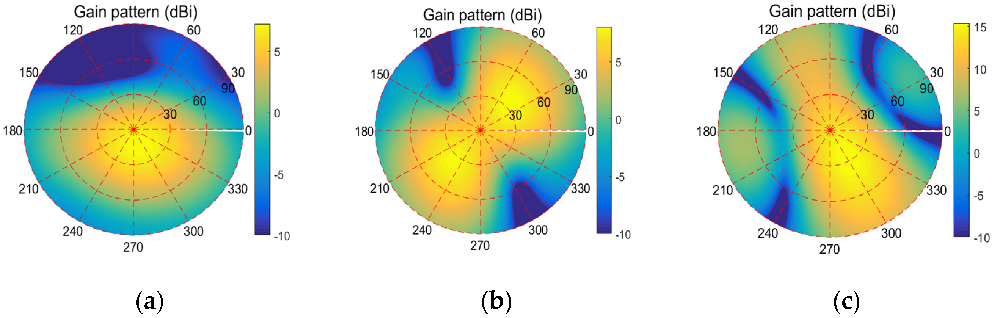
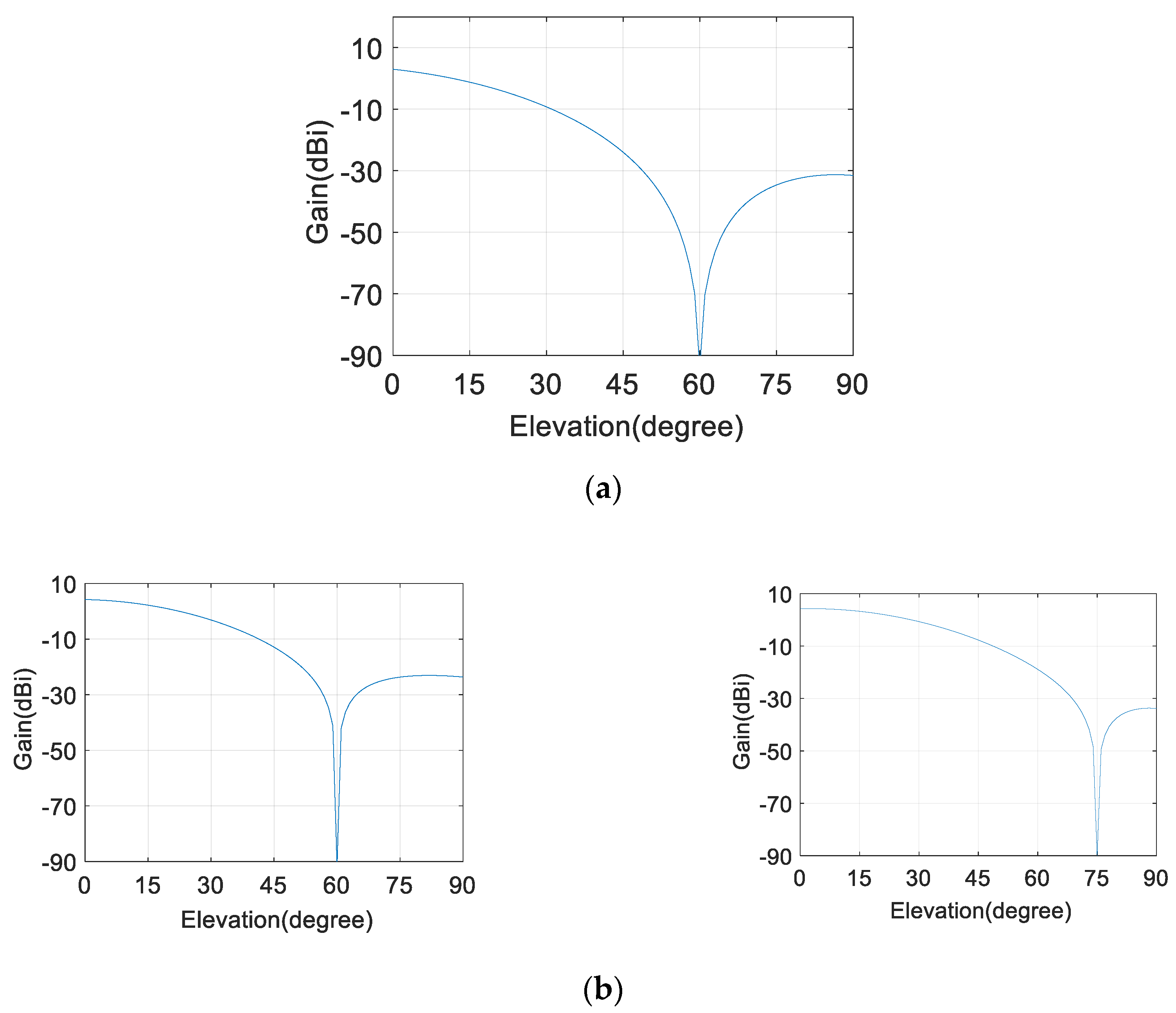
Figure 11 plots the adaptive gain of the four-element array (G1) towards the direction of the interferences in the specific scenes. Furthermore, the elements in the array are all selected as E1. As shown in
Figure 10, the nulling (about −90 dB) in the presence of one interference is much deeper than that (about −50 dB) when there are two or three interferences. This deeper nulling will cause the region where the adaptive array gain is less than the threshold to become much larger, as depicted in
Figure 12. On the other hand, the maximum array gains in
Figure 12a–c are 7.24 dB, 8.03 dB and 15.35 dB, respectively; that is, the array gain will be larger in a region far from the nulling as the number of RFIs increases. In summary, the availability will increase and the nulling capability will decrease as the number of RFIs increases.
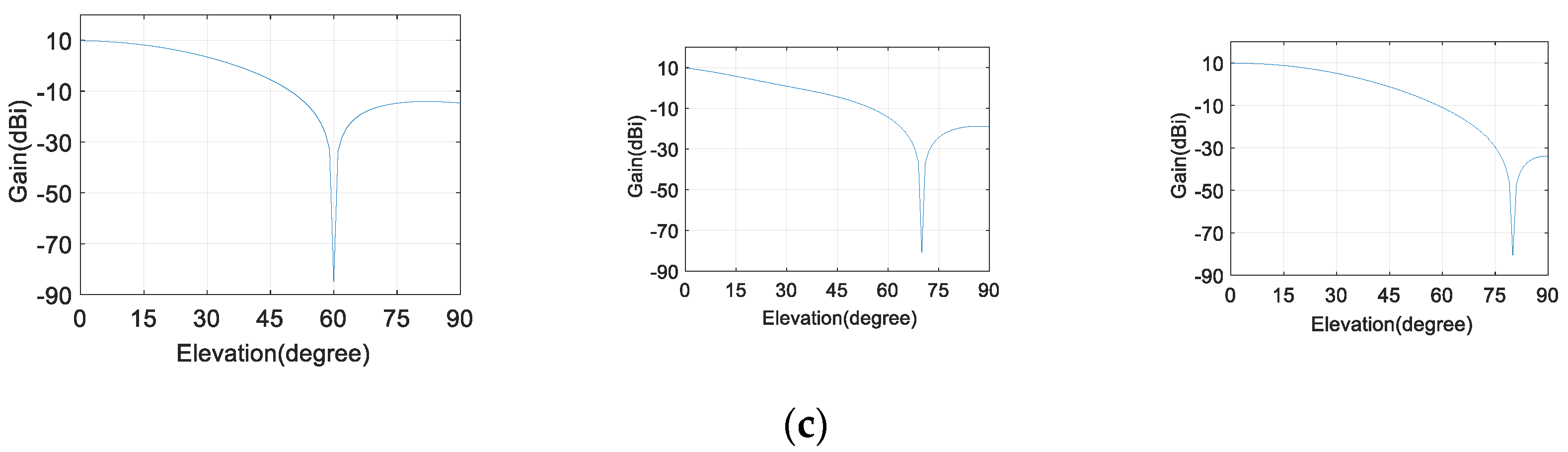
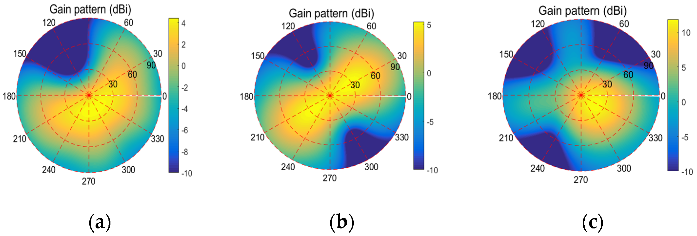
We suggest that the primary reason for this phenomenon may be the number of elements in the array being insufficient. We can improve the nulling capability by employing more elements in the array. As shown in
Figure 13, two more elements are added to the four-element array in
Figure 10 (other conditions are unchanged), and the nulling capability of the new six-element array did not decrease dramatically as the number of RFIs increased. In this case, the array gain and the availability obviously decreased, as depicted in
Figure 14, because the deeper nullings are steered as expected.
According to the analysis mentioned earlier, the availability sometimes cannot characterize the array performance comprehensively. The nulling capability may decrease when the availability improves; therefore, it is more meaningful to investigate the availability of antenna arrays with the same number of interferences and elements. Moreover, we should combine the null deepness and the availability to judge the performance of PI adaptive arrays so that we can investigate the antenna array comprehensively and fairly.


