Abstract
Misuse activity in computer networks constantly creates new challenges and difficulties to ensure data confidentiality, integrity, and availability. The capability to identify and quickly stop the attacks is essential, as the undetected and successful attack may cause losses of critical resources. The anomaly-based intrusion detection system (IDS) is a valuable security tool that is capable of detecting new, previously unseen attacks. Anomaly-based IDS sends an alarm when it detects an event that deviates from the behavior characterized as normal. This paper analyses the use of the histogram-based outlier score (HBOS) to detect anomalies in the computer network. Experimental results of different histogram creation methods and the influence of the number of bins on the performance of anomaly detection are presented. Experiments were conducted using an NSL-KDD dataset.
1. Introduction
With the increasing likelihood of becoming a target of malicious activity, it is necessary to take care of the security of information systems. Information systems are as secure as their weakest parts. In addition, there exists an inequality of efforts because only one vulnerability and one exploit are enough to compromise a system. In order to protect the information system, a complete set of security countermeasures has to be implemented. Therefore, it is very important to detect attacks at an early stage when the system has not been damaged yet. For this purpose, an intrusion detection system can be used. An intrusion detection system (IDS) is a union of hardware and software elements that monitors the system or network activity to identify and alert malicious events. There are two main approaches that are used for intrusion detection: signature-based and anomaly-based approaches. Signature-based IDS performs detections by comparing new data with the corresponding signature in the database of known attacks. Known attacks can be detected efficiently; however, new attacks are created every day, and in order to work efficiently, the system needs to be constantly updated with new signatures. The main drawback of the signature-based approach is that it fails to detect new, previously unseen attacks or even modified variants of known attacks.
Anomaly-based IDS operates on the assumption that the malicious activity is noticeably different from the normal system activity and, thus, is detectable. Anomaly-based IDS builds a model of normal network behavior, and any abnormal behavior that deviates from this model is marked as an intrusion. The main advantage of anomaly-based IDS is that it is capable of detecting new, previously unseen attacks. The main drawback is the high false alarm rate.
Goldstein and Uchida presented a comparative evaluation of various unsupervised anomaly detection algorithms [1]. The authors outlined the strengths and weaknesses of the algorithms with respect to their usefulness for specific applications. The nearest neighbor based algorithms performed better in most cases when compared to clustering algorithms, but the clustering-based algorithms had a lower computation time. The authors recommended using nearest neighbor based algorithms on datasets containing global anomalies and a local outlier factor (LOF) algorithm for local anomalies instead of clustering-based methods.
Anomalies can be detected using the feature-based anomaly detection approach by creating histograms of different traffic features [2]. In the proposed approach, anomalies are detected by modelling the detailed characteristics of constructed histograms and identifying deviations from the normal network traffic.
Perona et al. proposed network packet payload processing methodology based on histogram representations to detect anomalies [3]. They concluded that the payload analysis can be used in a general manner, with no service or port-specific modelling, to detect attacks in the network traffic.
Hofstede et al. also used packet payloads to detect brute-force attacks and compromised web applications [4]. The authors used clustering methods together with histograms of packet payload sizes to detect attacks. The Internet Protocol Flow Information Export (IPFIX) protocol was used to collect flow data.
A detailed review on methods for network anomaly detection was presented by Bhuyan et al. [5]. The authors described important aspects of the network anomaly detection, feature selection methods, and existing datasets. The paper concluded with important research issues, challenges, and recommendations for the developers of network anomaly detection methods and systems.
This paper analyses the use of a histogram-based outlier score (HBOS) to detect anomalies in the computer network. Experimental results of different histogram creation methods and the influence of the number of bins on the performance of anomaly detection using the NSL-KDD dataset are presented. The NSL-KDD dataset is a refined version of its predecessor, KDD99, and it is used to evaluate network-based intrusion detection systems [6].
2. Methodology
HBOS is a statistical anomaly detection algorithm [7]. HBOS calculates an outlier score by creating a univariate histogram for each single feature of the dataset. It assumes that features are independent. The drawback of assuming feature independence becomes less severe when the dataset has a high number of dimensions due to a larger sparsity [2]. The height of each single bin of the histogram represents the density estimation. To ensure an equal weight of each feature, the histograms are normalized in such a way that the maximum height of the bin would be equal to one. Then, calculated values are inverted so that anomalies have a high score and normal instances have a low score.
where d is the number of features, v is the vector of features, and histi(v) is the density estimation of each feature instance.
Three advantages of the HBOS include a fast computation time, scoring-based detection, and absence of a learning phase.
- The computation time is very significant, especially for computer networks where the amount of data that needs to be analyzed to detect anomalies is very large. HBOS is up to 5 times faster than clustering-based algorithms and up to 7 times faster than nearest-neighbor based methods [7].
- In the anomaly detection, scoring-based detection methods assign an outlier score to each of the data points. This is an advantage compared to binary output methods because, additionally, the outlier score allows estimating the reliability or certainty of the prediction.
- HBOS is an unsupervised method; therefore, it has no training or learning phase and does not require data labelling. The only parameter that needs to be specified is the number of bins of the histogram.
Two different methods can be used to construct histograms: the static bin width or the dynamic bin width. In the first case, data are grouped using bins of the same width. A rectangle is drawn in each interval whose height is proportional to the number of points that fall into the interval. Equal binning assumes that each bin is equally likely, but this assumption is usually not met. Using dynamic bins, the width of bins depends on the values of data and may not necessarily be equal to the specified number of bins. In the case of long-tail distributions with repetitive integers, some bins may contain more values than specified. In both static and dynamic cases, it is necessary to specify the number of bins k. It is recommended that the k value should be equal to the square root of all data points.
It is important to note that in applying dynamic bins to construct histograms, in cases where the selected number of bins k is greater than the number of unique values of the feature, the number of bins will be equal to the number of unique values. It can be illustrated using a simple numeric example with a set of 12 integers {1,9,1,1,2,1,1,9,1,2,1,1}. After applying dynamic bins with k = 4, the resulting bins are {1,1,1,1,1,1,1,1}, {2,2}, and {9,9}. If k = 2, the processing steps are as follows:
- the data are split into two intervals with the same quantity of values {1,1,1,1,1,1} and {1,1,2,2,9,9};
- if the maximum value of the first bin is not equal to the minimum value of the second bin, this value moves from the second bin to the first one. Repeat step 2 until all bins are checked. The resulting bins would be {1,1,1,1,1,1,1,1} and {2,2,9,9}.
The number of bins will be equal to the selected k only when the number of unique values of the feature is greater than or equal to k.
The HBOS anomaly detection algorithm was implemented using R programming language. R is a scripting language for statistical data analysis and visualization.
For the experiment, we used the NSL-KDD dataset [6]. The NSL-KDD dataset is a refined version of its predecessor, KDD99, and has the following advantages: it does not include redundant and duplicated instances, and the number of available instances in the train and test datasets are reasonable; therefore, it is possible to execute experiments with the complete set. Each instance of the NSL-KDD dataset contains 41 main features (e.g., duration, protocol type, service) and 2 additional features describing the type and the difficulty level of each instance.
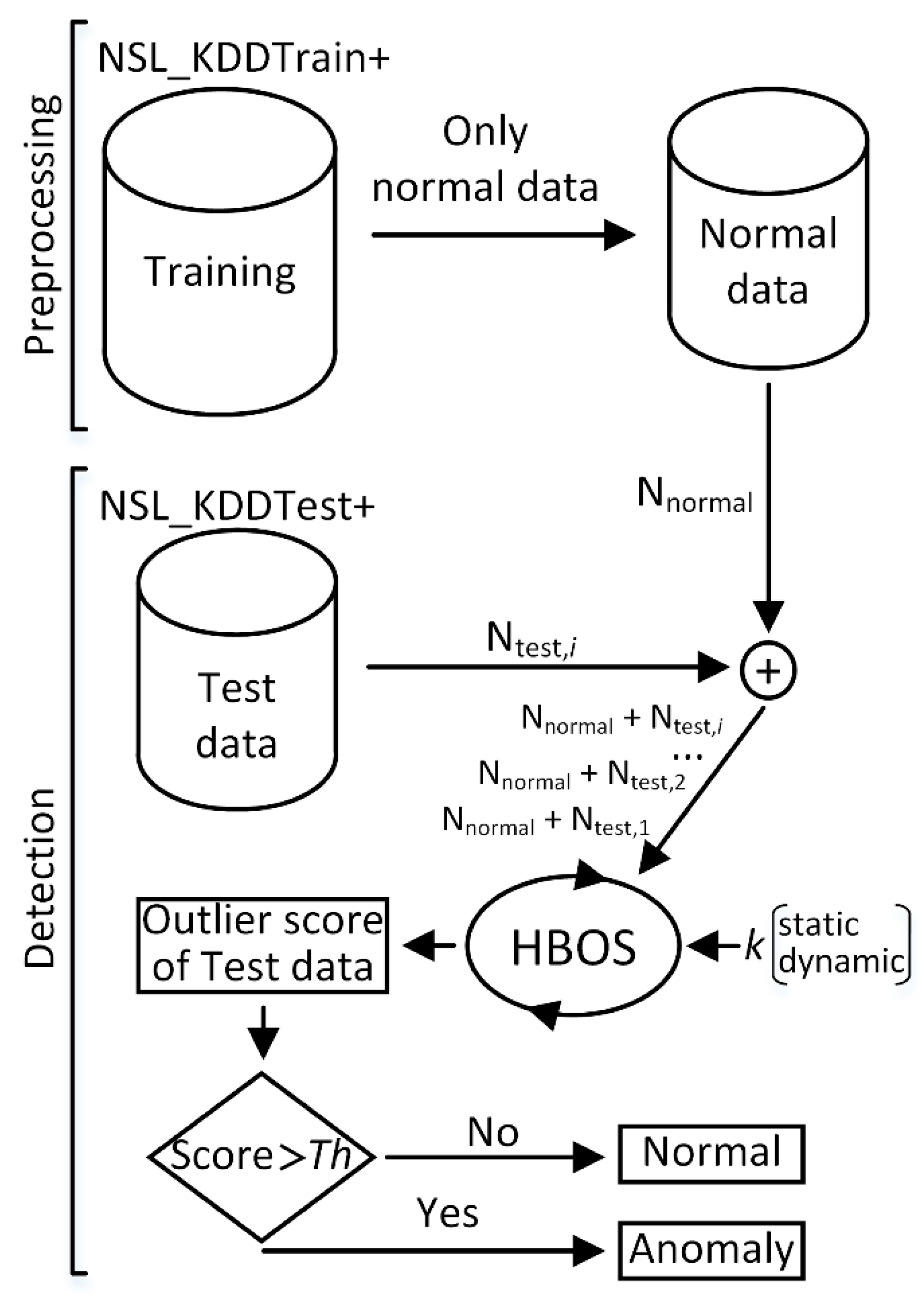
Figure 1 illustrates the anomaly detection process consisting of two steps: data preprocessing and anomaly detection. The first step splits NSL-KDD training data into normal and attack datasets. Only training data labelled as normal were used in the anomaly detection step, which consisted of 67,343 instances. In a real-world scenario, it is much easier to collect data corresponding to normal network behavior rather than data with a complete set of possible attack types. In computer networks, the number of normal packets is significantly larger than anomalous ones. After the data preprocessing step, the resulting dataset is further used to detect anomalies. This dataset is accompanied by a new instance from the test dataset. The NSL-KDD test data set consisted of 22,544 instances, from which 9711 were labelled as normal, and 12,833 instances were assigned to one of four attack types: denial-of-service (DOS, 7458), surveillance and other probing (PROB, 2421), unauthorized access from a remote to local host (R2L, 2887), and unauthorized access to the local super user (U2R, 67). HBOS was applied with the specified number k and the type of bins. The tested instance was flagged as an anomaly if its HBOS value exceeded an estimated threshold Th.
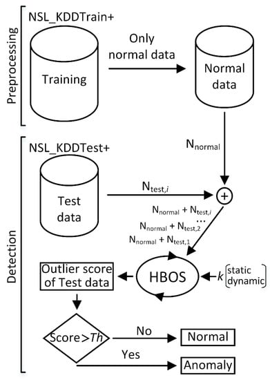
Figure 1.
Data preprocessing and anomaly detection scheme. HBOS, histogram-based outlier score; NSL_KDD.
3. Experimental Results and Discussion
Experiments were conducted using static and dynamic histogram construction methods with different numbers of bins k. Table 1 shows unique values of each feature of NSL-KDD in training normal data. When using the recommended number of bins, k is equal to the square root of all data points (k = sqrt (67,343 + 1) ≈ 259). It can be seen that each unique value of 36 features will fall into separate bins, and the values of only 5 remaining features (features 1, 5, 6, 23, and 24) will be grouped into selected bins. To evaluate the influence of grouping on the performance of anomaly detection, it is reasonable to try different k values. A lower k value will increase the influence of grouping, whereas a higher k value will decrease it.

Table 1.
Unique values of features of NSL-KDD in training normal data.
F-measures were used for to evaluate the performance of anomaly detection. The F-measure represents the balance between precision (P) and recall (R): (2 × P × R / (P + R)) [5]. The F-measure ranges from 0 to 1, where 1 is an ideal case. Precision is defined as the ratio between the number of correctly detected anomalies and the total number of detected anomalies (TP / (TP + FP)), where TP is the true positive and FP is the false positive. Recall is defined as the ratio between the number of correctly detected anomalies and the total number of anomalies (TP / (TP + FN)), where FN is the false negative.
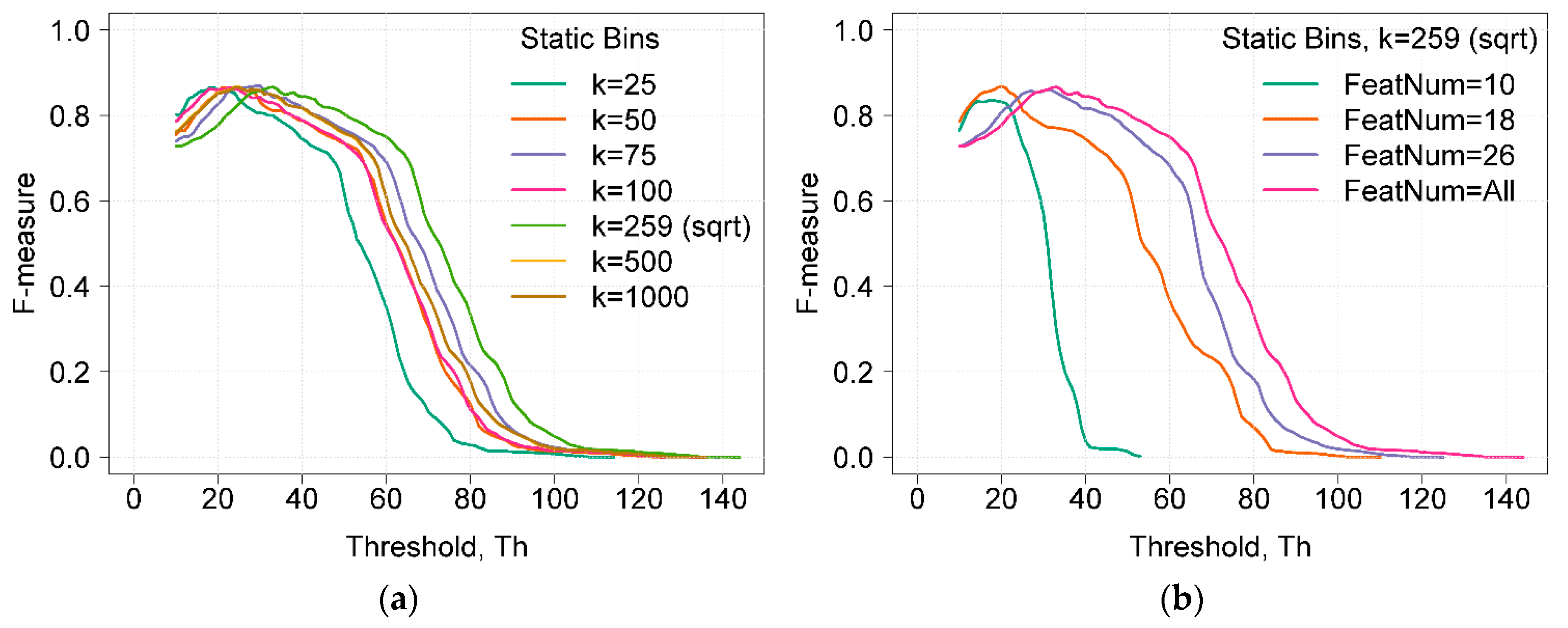
Figure 2a shows the dependences of F-measure on the detection threshold Th using static bins and a different number of k bins. The maximum value of the F-measure did not depend on the number of selected k bins, and it reached 0.86. However, the number of k bins influenced the width and position of the curve at the maximum value of the F-measure. A higher curve width indicates better results, as the attack detection is less dependent on the threshold value. The width of the curves can be compared by choosing a reference point of the F-measure. If the chosen reference point was 0.8 (i.e., the F-measure value was higher than 0.8), the range of threshold values was 23 units (from 10 to 33) when k = 25. The widest range was equal to 29 units and was reached when k was equal to or higher than 259. As a result, the maximum value of the F-measure did not change, but the width of the curve changed when k increased (when the influence of the grouping value was lowered).

Figure 2.
(a) Dependence of the F-measure on the detection threshold Th using static bins and a different number of bins k. (b) Dependence of the F-measure on the detection threshold Th using static bins at different feature sets.
Figure 2b illustrates the dependence of the F-measure on the detection threshold Th using static bins with a different set of features. Feature sets were selected based on the results proposed by other authors. Zargari et al. proposed to use a feature set composed of 10 features (FeatNum = 10) obtained using Weka by applying the InfoGainVal+Ranker method [8]. Ambusaidi et al. suggested to use a set of 18 features. For feature selection, they proposed the Flexible Mutual Information Based Feature Selection (FMIFS) algorithm [9]. The feature set composed of 26 features is proposed in [10].
It can be seen that when applying HBOS with only 10 features, the maximum F-measure was 0.83 and the range of threshold values was only 11 units. With 18 features, the maximum F-measure was 0.86 and the range was 15 units. The lower threshold range, where the F-measure was higher than 0.8, indicates that the difference between the normal score and the anomaly score is lower. When using a set of 26 features, the maximum value of the F-measure was 0.86 and the threshold range was 26 units (from 20 to 46) (i.e., only 3 units lower compared to the case when all features were used). Applying HBOS with a set of 26 features looks promising because less features mean a shorter computation time. When using only 26 features, the computation time was about 34 % shorter as compared to the computation time when all features were used.
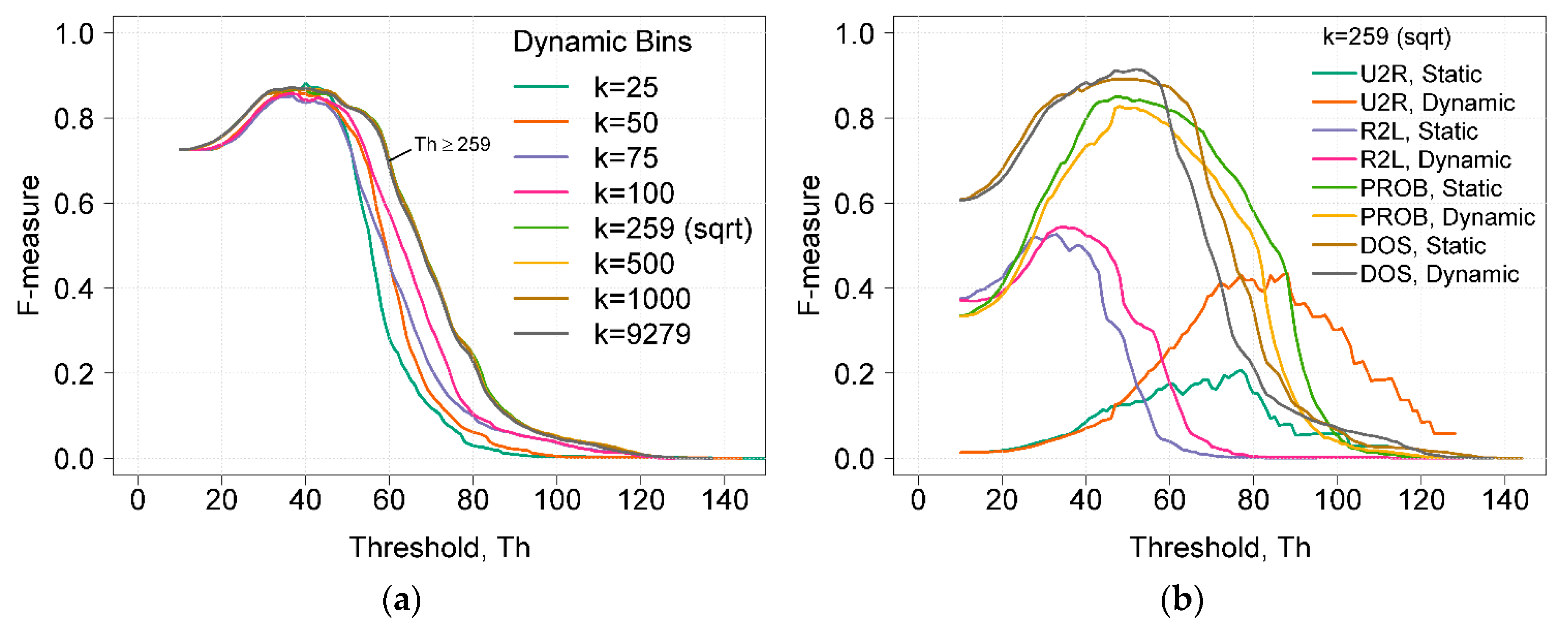
Figure 3a shows the dependences of the F-measure on the detection threshold Th using dynamic bins and a different number of k bins. By analyzing the F-measure values when using the dynamic bins with different k values, it can be seen that the F-measure results obtained were very similar, and only the curve widths were different (Figure 3a). Using k values higher than the square root of all data points did not influence anomaly detection. When k = 259, only five feature values (1, 5, 6, 23, and 24) having a higher unique value were grouped. When k was equal to the maximum possible number of unique values (k = 9279), the influence of grouping values was eliminated.
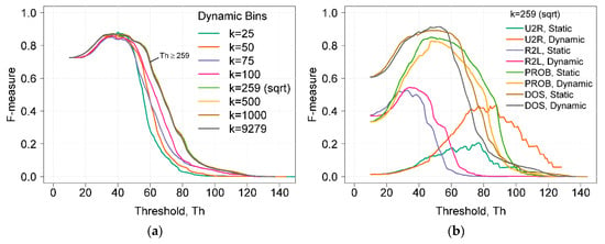
Figure 3.
(a) Dependence of the F-measure on the detection threshold Th using dynamic bins and different numbers of bins k. (b) Comparison of F-measure results obtained by using static and dynamic histogram construction methods.
Figure 3b shows a comparison of F-measure results of different attack types. Results were obtained using static and dynamic histogram construction methods with k = 259. It was seen that the F-measure results of U2R attacks differed the most. When using dynamic bins, the calculated HBOS values of U2R attacks were higher. This fact increased the threshold and improved the precision of attack detection. The ability to detect U2R attacks is very important because this type of attack may cause the greatest harm to the system. Small F-measure values of U2R were due to a very low number of these attacks (only 67, compared to 67,343, the total number of instances); therefore, even a small number of false positives significantly influences the results. F-measure values obtained using dynamic bins showed better results in three (U2R, R2L, and DOS) out of four attack types; therefore, the overall performance was better compared to F-measure results using static bins.
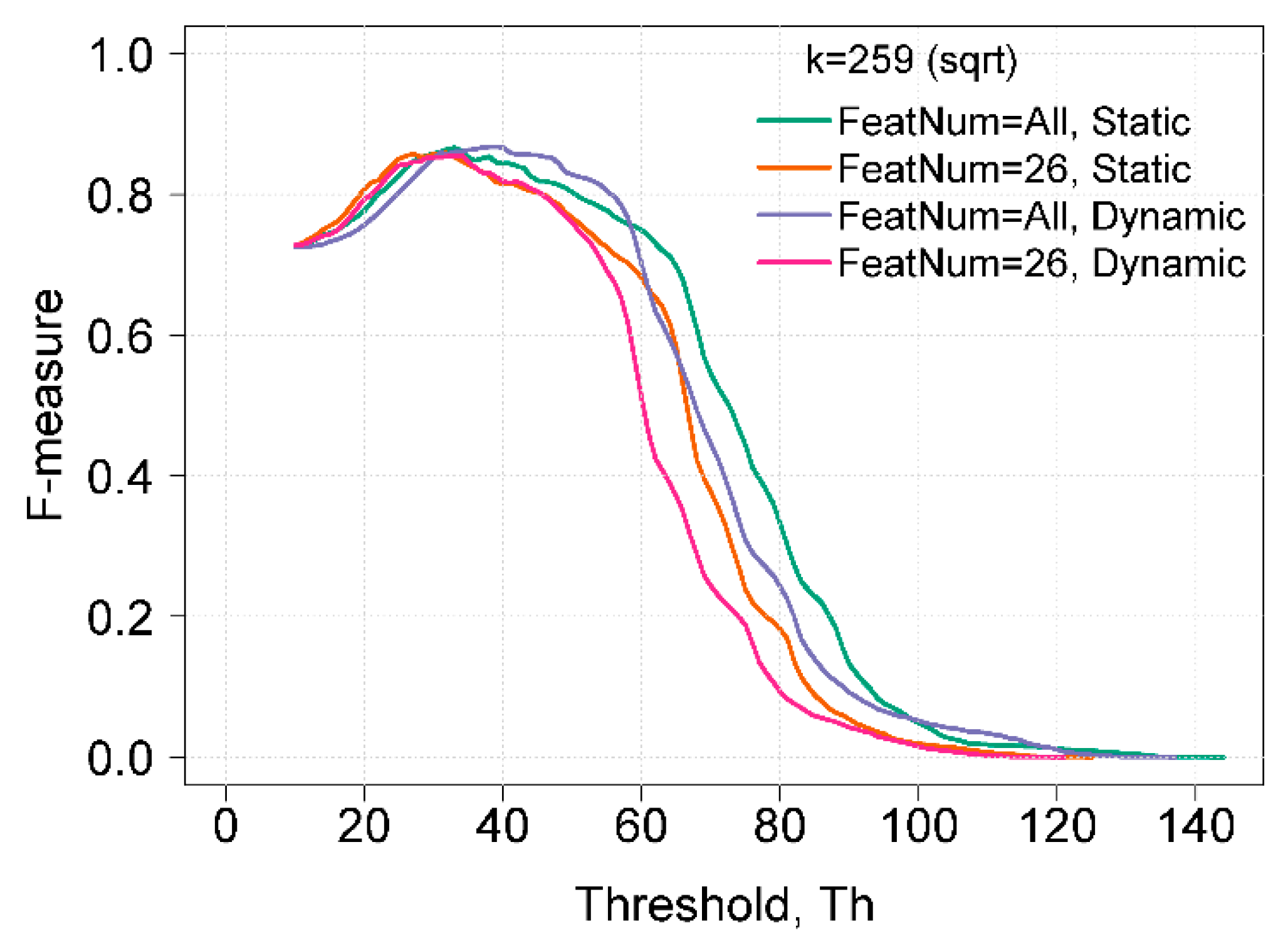
Figure 4 shows a comparison of the best F-measure results obtained using static and dynamic histogram construction methods. In using a set of 26 features for both static and dynamic bins, the maximum F-measure was 0.86 with Th = 34. A reduced feature set is recommended for use when a shorter computation time is preferred, as the influence on the results of anomaly detection is not significant, but the reduction in computation time is tangible. The overall best results of the F-measure were obtained using dynamic bins and all features. In this case, the maximum F-measure was 0.87 with Th = 39. The range, when the F-measure was equal or higher than 0.86, was from 31 to 41, whereas when using static bins, the range was from 30 to 34.
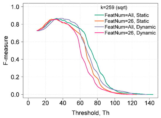
Figure 4.
Comparison of F-measure results using different histogram construction methods and feature sets.
A comparison of results based on the NSL-KDD dataset with other approaches [11,12,13,14,15] is listed in Table 2. The application of HBOS with dynamic bins showed better results compared to other related methods, especially those detecting R2L and U2R types of attacks.

Table 2.
Comparison of F-measure results with related works.
4. Conclusions
In this paper, the histogram-based outlier score was implemented to detect anomalies in the computer network. The maximum F-measure value (0.87 with Th = 39) in anomaly detection was not significantly dependent on the chosen histogram construction method. The number of bins mainly influenced the width of the F-measure curve at the maximum value. A higher curve width indicates better results, as the attack detection is less dependent on the threshold value, and it also means that the difference between the anomaly score and the normal score is higher. The higher number of bins reduces the influence of data grouping. The unique values of the most important (most predictive power) features can be used as the reference point to select the number of bins.
F-measure values obtained using dynamic bins showed better results in three out of four attack types; therefore, the overall performance was better compared to F-measure results using static bins. In addition, HBOS with dynamic bins showed better results in detecting rare events (i.e., U2R attacks).
Author Contributions
Conceptualization, N.P. and A.B.; Investigation, N.P.; Validation, A.B.; Writing—original draft, N.P.; Writing—review & editing, N.P. and A.B.
Funding
This research received no external funding.
Conflicts of Interest
The authors declare no conflicts of interest.
References
- Goldstein, M.; Uchida, S. A Comparative Evaluation of Unsupervised Anomaly Detection Algorithms for Multivariate Data. PLoS ONE 2016, 11, e0152173. [Google Scholar] [CrossRef] [PubMed]
- Kind, A.; Stoecklin, M.P.; Dimitropoulos, X. Histogram-based traffic anomaly detection. IEEE Trans. Netw. Serv. Manag. 2009, 6, 110–121. [Google Scholar] [CrossRef]
- Perona, I.; Albisua, I.; Arbelaitz, O.; Gurrutxaga, I.; Martin, J.; Muguerza, J.; Pérez, J.M. Histogram based payload processing for unsupervised anomaly detection systems in network intrusion. In Proceedings of the 14th Portuguese Conference on Artificial Intelligence, Aveiro, Portugal, 1 October 2019; pp. 329–340. [Google Scholar]
- Hofstede, R.; Jonker, M.; Sperotto, A.; Pras, A. Flow-Based Web Application Brute-Force Attack and Compromise Detection. J. Netw. Syst. Manag. 2017, 25, 735–758. [Google Scholar] [CrossRef]
- Bhuyan, M.H.; Bhattacharyya, D.K.; Kalita, J.K. Network anomaly detection: Methods, systems and tools. IEEE Commun. Surv. Tutor. 2014, 16, 303–336. [Google Scholar] [CrossRef]
- Tavallaee, M.; Bagheri, E.; Lu, W.; Ghorbani, A. A Detailed Analysis of the KDD CUP 99 Data Set. In Proceedings of the Second IEEE Symposium on Computational Intelligence for Security and Defense Applications (CISDA), Ottawa, ON, Canada, 8–10 July 2009. [Google Scholar]
- Goldstein, M.; Dengel, A. Histogram-based outlier score (HBOS): A fast unsupervised anomaly detection algorithm. In KI-2012: Poster and Demo Track; Wölfl, S., Ed.; Citeseer: Princeton, NJ, USA, 2012; pp. 59–63. [Google Scholar]
- Zargari, S.; Voorhis, D. Feature Selection in the Corrected KDDdataset. In Proceedings of the 2012 Third International Conference on Emerging Intelligent Data and Web Technologies, Bucharest, Romania, 19–21 September 2012; pp. 174–180. [Google Scholar]
- Ambusaidi, M.A.; He, X.; Nanda, P.; Tan, Z. Building an intrusion detection system using a filter-based feature selection algorithm. IEEE Trans. Comput. 2016, 65, 2986–2998. [Google Scholar] [CrossRef]
- Aziz, A.S.A.; Azar, A.T.; Salama, M.A.; Hassanien, A.E.; Hanafy, S.E.O. Genetic Algorithm with Different Feature Selection Techniques for Anomaly Detectors Generation. In Proceedings of the Federated Conference on Computer Science and Information Systems (FedCSIS 2013), Kraków, Poland, 8–11 September 2013; pp. 769–774. [Google Scholar]
- Divekar, A.; Parekh, M.; Savla, V.; Mishra, R.; Shirole, M. Benchmarking datasets for anomaly-based network intrusion detection: KDD CUP 99 alternatives. In Proceedings of the IEEE 3rd International Conference on Computing, Communication and Security (ICCCS), Kathmandu, Nepal, 25–27 October 2018; pp. 1–8. [Google Scholar]
- Javaid, A.; Niyaz, Q.; Sun, W.; Alam, M. A deep learning approach for network intrusion detection system. In Proceedings of the 9th EAI International Conference on Bio-inspired Information and Communications (BICT), New York, NY, USA, 3–5 December 2015; pp. 21–26. [Google Scholar]
- Alguliyev, R.; Aliguliyev, R.; Sukhostat, L. Anomaly Detection in Big Data based on Clustering. Stat. Optim. Inf. Comput. 2017, 5, 325–340. [Google Scholar] [CrossRef]
- Potluri, S.; Diedrich, C. Deep Feature Extraction for Multi-class Intrusion Detection in Industrial Control Systems. Int. J. Comput. Theory Eng. IJCTE. 2017, 9, 374–379. [Google Scholar] [CrossRef]
- Wahyudi, B.; Ramli, K.; Murfi, H. Implementation and Analysis of Combined Machine Learning Method for Intrusion Detection System. Int. J. Commun. Netw. Inf. Secur. (IJCNIS) 2018, 10, 295–304. [Google Scholar]
© 2019 by the authors. Licensee MDPI, Basel, Switzerland. This article is an open access article distributed under the terms and conditions of the Creative Commons Attribution (CC BY) license (http://creativecommons.org/licenses/by/4.0/).

