Abstract
Target recognition is an important area in Synthetic Aperture Radar (SAR) research. Wide-angle Synthetic Aperture Radar (WSAR) has obvious advantages in target imaging resolution. This paper presents a vehicle target recognition algorithm for wide-angle SAR, which is based on joint feature set matching (JFSM). In this algorithm, firstly, the modulus stretch step is added in the imaging process of wide-angle SAR to obtain the thinned image of vehicle contour. Secondly, the gravitational-based speckle reduction algorithm is used to obtain a clearer contour image. Thirdly, the image is rotated to obtain a standard orientation image. Subsequently, the image and projection feature sets are extracted. Finally, the JFSM algorithm, which combines the image and projection sets, is used to identify the vehicle model. Experiments show that the recognition accuracy of the proposed algorithm is up to 85%. The proposed algorithm is demonstrated on the Gotcha WSAR dataset.
1. Introduction
Synthetic Aperture Radar (SAR) has excellent imaging ability, which can obtain high-resolution image under bad weather conditions. The research on SAR includes imaging, target detection, target recognition, time-frequency analysis, and many other aspects [1,2,3,4,5,6,7,8]. The research on Automatic Target Recognition (ATR) of SAR started around 1990 [9,10,11]. ATR is still one of the most challenging research topics. Many researchers have conducted excellent research on SAR ATR [12,13,14].
Wide-angle Synthetic Aperture Radar (WSAR) is a type of the Synthetic Aperture Radar (SAR). Franceschetti et al. introduced the acquisition model and algorithms for the precision processing of SAR data with a large slant range dimension in the early 1990s [15,16]. Different researchers have studied the imaging methods and scattering center models of WSAR [17,18,19,20,21,22,23,24]. Moses et al. gives a definition of WSAR, which refers to any synthesized aperture whose angular extent exceeds the sector that is required for equal resolution in range and cross-range [25]. In 2007, Air Force Research Laboratory (AFRL) released the first Gothca dataset and challenge problem [26]. Subsequently, Dungan et al. proposed several discrimination algorithms for the challenge problem [27,28,29]. In 2012, Dungan et al. worked with AFRL to process the Gothca dataset. They tailored and separated the small data of 33 civilian vehicles from the big scene, and numbered them according to vehicle type and radar detection height, respectively. They published Target Discrimination Research Challenge and the corresponding data subset [30]. Subsequently, different researchers have studied WSAR target recognition [31,32,33,34,35].
The idea of combining imaging and target detection has been studied in the field of infrared target detection [36,37,38,39,40]. This paper introduces an imaging method that is more beneficial in target recognition. Based on the backprojection imaging algorithm, the modulus stretch transform function is added to the imaging process. The image after processing has thinner contour edges than that obtained from the traditional backprojection algorithm. After obtaining contour image, the gravitational-based speckle reduction algorithm is used to obtain a clearer contour image. Subsequently, the image is rotated to obtain a standard orientation image. Accordingly, the image and projection feature set can be extracted from these processed images. Finally, the joint feature set matching (JFSM) algorithm is used to identify the vehicle model. Figure 1 displays an outline of the proposed algorithm.
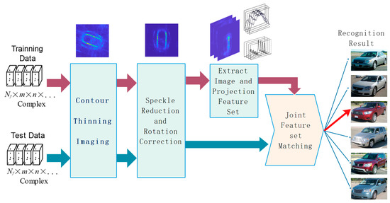
Figure 1.
The outline of the proposed joint feature set matching (JFSM) algorithm.
2. Contour Thinning Imaging
The contour thinning imaging algorithm is an improved algorithm based on the backprojection algorithm. The principle and steps of contour thinning imaging algorithm are described in detail in Reference [35]. In this paper, the main steps of the algorithm are given below.
According to the principle of SAR detection, the radar transmits a linear continuous frequency modulation wave to the target and it receives the echo by matched filter. Radar echo data are functions of receiving frequency f and slow time which is denoted by . In practice, echo data are discretized data, so they are often rewritten as , where denotes the k-th sampling frequency and denotes the n-th sampling slow time.
- The -point IFFT transform is performed on the echo data received at each slow time to obtain an M-point inverse transform sequence, and it is then cyclically shifted with the FFTshift (•) function.
- Let denote the target coordinates in the detection scene. Let denote the difference between the distance from the sensor to the origin and the distance from the sensor to the target with the coordinate r at time Linear interpolation is performed on to obtain the estimated values of the corresponding IFFT transformation at all points and the sub-imaging data at each time is obtained by multiplying the data with the compensation term.where L denotes the real side length of the imaged scene. Let denotes the distance of the antenna from the origin of the ground at coordinate r and the time . Let denotes the distance of the antenna from the target in the ground. is calculated, as follows.
- Let denote the value of the synthetic aperture. The sub-images of all in the range of the synthetic aperture are superimposed, and the modulus is then stretched for each sub-aperture image by using the function. Finally, all of the sub-aperture images are superimposed to obtain the final image I.where T is the threshold value, is the enhancement coefficient, and is the inhibition coefficient.
Figure 2 shows an example of imaging results for four different models. Figure 2a–d are the imaging results of using the traditional backprojection algorithm for four models of vehicles, namely Chevrolet Impala LT, Mitsubishi Galant ES, Toyota Highlander, and Chevrolet HHR LT. Figure 2e,f correspond to Figure 2a–d for the contour thinning imaging result. The synthetic aperture is 10°. According to Reference [35], the parameters of the modulus stretch function were = 1.2, = 0.1, and T = 0.9. It can be seen that the image of all models of vehicles after modulus stretch greatly strengthens the contour features of the target.
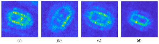
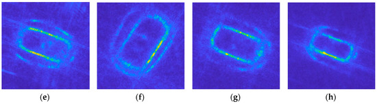
Figure 2.
Example of imaging results of different models of vehicle targets in the Gotcha dataset by contour thinning imaging: (a,e) Chevrolet Impala LT; (b,f) Mitsubishi Galant ES; (c,g) Toyota Highlander; and, (d,h) Chevrolet HHR LT.
3. Speckle Reduction and Rotation Correction
3.1. Speckle Reduction
Although the image after contour thinning is clearer than before, there are still some noise and artifacts. We use the speckle reduction algorithm commonly used in SAR target detection in order to reduce these noises and artifacts. There are many different speckle reduction algorithms that work well in certain scenarios. The gravitation-based speckle reduction algorithm [41,42] has excellent denoising and anti-artifact effects, so it is used to process the above images.
The algorithm treats the relationship between the target pixel and the speckle pixel as a gravitation relationship. Pixels that are near the target pixel are also more likely to be target pixels, which is proportional to their own brightness and the number of target pixels around that pixel, and inversely proportional to the distance between the pixel and other target pixels. Therefore, the concept of gravitation is introduced to describe the interaction between pixels. The two-dimensional SAR image is regarded as a two-dimensional gravitational field. Different pixels represent different objects in the gravitational field. The gravitation-based speckle reduction algorithm is calculated, as follows:
where I(i, j) and I(k, l) represent the brightness at coordinates (i, j) and (k, l) on image I. , represents the distance between (i, j) and (k, l). R is the radius of gravitational action. The value of R is related to the size of the target. If R is too small, the target will not be enhanced, while, if R is too large, the noise will also be enhanced. From the experimental results, the value of R can be taken as 1/10 of the target size. m is the coefficient of gravitation. In general, the value of m is taken as 1. G(i, j) represents the gravitational pull of the surrounding pixels that are received by the pixel (i, j). F(i, j) represents the internal stress of the pixel (i, j) itself. The final enhanced pixel brightness I’(i, j) is the sum of the gravitation around the pixel and its internal stress.
Figure 3 shows the example of results after the gravitation-based speckle reduction algorithm of Figure 2e–h. In this case, the radius of gravitational action R is 10 and the coefficient of gravitation m is 1.
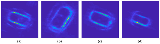
Figure 3.
Example of results after the gravitation-based speckle reduction algorithm of Figure 2e–h. The corresponding vehicle models are: (a) Chevrolet Impala LT; (b) Mitsubishi Galant ES; (c) Toyota Highlander; and, (d) Chevrolet HHR LT.
3.2. Rotation Correction
In the actual scene, there is no limit to the parking direction of the vehicle, so the vehicle direction angle on the SAR image is also uncertain. The image obtained by backprojection and other traditional imaging algorithms have blurred contour, which is complex and difficult to automatically detect the rotation angle of the vehicle. In the matching algorithm used in Reference [26,27,28,29], vehicle rotation angle is considered as a variable to be added to the equation together with other parameters, and the specific optimization algorithm solves all unknown variables. However, after using the contour thinning imaging and speckle reduction algorithm, clear vehicle contour lines can be obtained, and Hough transform algorithm can be used to detect the contour line, so as to calculate the vehicle rotation angle. The Hough transform is a very common algorithm that is used to detect straight lines in the field of image processing, which is described in detail in Reference [43], and it will not be repeated in this paper.
The contour image is firstly processed by edge detection algorithm to obtain the binarized edge image in order to accurately detect the contour line. Subsequently, the hough transform is used to detect the straight line to obtain the rotation angle of the vehicle. Edge detection operators can use simple operators such as Sobel, which is calculated, as follows:
where and are horizontal and vertical Sobel operators, I is the original image, and is the edge image. The symbol * represents a convolution operation.
After obtaining the vehicle rotation angle θ, the image can be corrected by the rotation transformation equation. The point in the original image whose coordinates are (x, y) is changed to (x′, y′) after transformation. The transformation equation is as follows:
It should be noted that the origin is not in the center when the image is taken as matrix data. Therefore, the origin should be moved to the center before rotation and then restored after rotation. Figure 4 shows the three steps of rotation correction while using Figure 3a as an example.
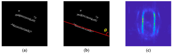
Figure 4.
The three steps of rotation correction using Figure 3a as an example. (a) Edge detection is performed; (b) The Hough transform is used to detect the straight line to obtain the angle θ between the vehicle and the vertical direction; and, (c) The original image is rotated by θ to make the vehicle in the vertical direction.
4. Feature Set Extraction and Matching
After the previous processing, the obtained image is used for feature set extraction. It can be seen from Figure 2a–d that the image obtained by the traditional backprojection algorithm is fuzzy, and it is difficult to directly extract the shape, contour, and other features of the vehicle. After contour thinning and speckle reduction, the vehicle contour is much clearer than before, and it is convenient to detect the contour line, calculate the rotation angle of the vehicle, and other contour data. In this paper, a vehicle recognition algorithm that is based on combined matching of contour image feature set and orthogonal projection feature set is proposed.
4.1. Feature Set Extraction
Figure 5 shows an example of the imaging results for four different models of vehicle at different positions and detection heights. These images have been pre-processed by contour thinning, speckle reduction, and rotation correction. Figure 5a–d are images of the vehicle model Chevrolet Impala LT. Figure 5e–h are images of the vehicle model Mitsubishi Galant ES. Figure 5i–l are images of the vehicle model Toyota Highlander. Figure 5m–p are images of the vehicle model Chevrolet HHR LT.
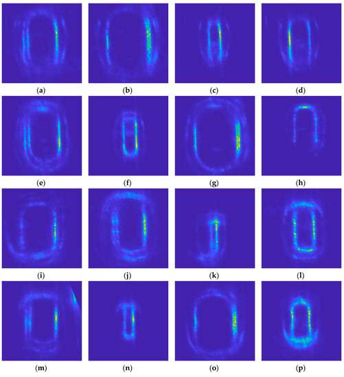
Figure 5.
Example of imaging results for four different models of vehicle at different positions and detection heights. (a–d) Chevrolet Impala LT; (e–h) Mitsubishi Galant ES; (i–l) Toyota Highlander; and, (m–p) Chevrolet HHR LT.
It can be seen from Figure 5 that different contour sizes of the same model will appear when imaging in different detection locations and different detection heights. Moreover, the contours of different models are sometimes very similar and, in some cases, are more similar than the contours of the same model. Therefore, if only a simple size feature, such as the length or width of the contour, is used, it is difficult to recognize the model of the vehicle. Accordingly, we consider establishing a feature set for each model for recognition. The feature set consists of two parts, one is the selected image data set and the other is the projection data set.
4.1.1. Selected Image Set
Template matching is a simple and direct method for image classification. The matching value can be calculated between the contour image to be recognized and the image in the existing image set and then the category of the image with the largest matching value can then be taken as the vehicle recognition result. Obviously, the more images in the image set and the more representative the images are, the higher the recognition accuracy is. In extreme cases, if the image set contains all of the known images, then the highest recognition accuracy should ideally be achieved. However, in reality, the image set cannot contain all the images, because the actual images are endless, and there will always be new images that have not appeared. Moreover, the image set containing all images loses the significance of studying representative features, and it becomes unnecessarily large and redundant.
Therefore, this paper proposes a simple image set generation algorithm. The algorithm can preserve as many representative images as possible and remove redundant images as possible. Let K denote the total number of known contour images and denote the k-th contour image. Let N denote the number of vehicle models and indicate the i-th model. For any contour image , there is , where . Let denote the image set corresponding , and the steps for generating the image set are as follows:
- All images belonging to are added to the image set , and an image is then randomly selected from as the reference image .
- The correlation coefficients C of and all other model of images is calculated. The minimum Cmin of correlation coefficients C is obtained. The equations are as follows:where is the mean of the I. represents the correlation coefficient of the overlapping region with Ii, when Ij is shift to (u, v), so the mean value is also the mean value of the overlapping region.
- The correlation coefficients of and all of the images in are calculated, and the image with the correlation coefficient smaller than is removed from .
- A new image is randomly selected from as the reference image , and then Step 2–4 are repeated. If all the images in have been reference images, the algorithm ends. Finally, is the generated image set.
The image set corresponding to each model can be obtained by following the above steps for all models.
4.1.2. Projection Set
The image set that was obtained after selection process retains some representative images, but many images are also removed, and some features of this model are inevitably lost. In order to compensate for the feature loss, the orthogonal projection feature of the image is saved to increase the recognition accuracy. The horizontal projection and vertical projection have obvious characteristics because the image has been rotated before. Additionally, since the projection data is much smaller than the image data, it is very convenient and cost-effective to store the projection features, and the projection features of all the images can be saved. The horizontal and vertical projection of the image is calculated, as follows:
Figure 6 shows the example of the horizontal projection curve and the vertical projection curve of Figure 5a. The image size is 200 × 200.
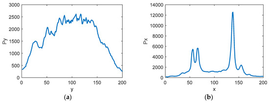
Figure 6.
Example of the horizontal projection curve and the vertical projection curve of Figure 5a. (a) Horizontal projection curve; (b) Vertical projection curve.
The orthogonal projection feature set of each model can be obtained by saving the horizontal and vertical projection data of all images of each model.
4.2. Joint Feature Set Matching
The JFSM algorithm can be carried out after obtaining the image set and projection set. Define the maximum value of the correlation coefficient of two objects as their matching value :
Equations (15) and (16) show the calculation of the correlation coefficient . The correlation coefficients between the image to be recognized and each image in the image set of each model was calculated, and the maximum of the correlation coefficients was taken as the image matching value with the model. Similarly, the horizontal and vertical projections of the image to be recognized were calculated, and the correlation coefficients were calculated with the projection sets of each model, and the maximum values of them were respectively taken as the projection matching values and . The final overall matching degree is obtained by the weighted combination of the above three matching values:
where α is the weight, which indicates the importance of image matching value in the overall matching degree. The above equation only calculates the matching degree of one model. In practice, it needs to calculate the matching degree of all models. Finally, the model corresponding to the maximum matching degree is the recognition result of the vehicle.
5. Experimental Results
The Target Discrimination Research subset of the Gotcha dataset that was published by the Air Force Research Laboratory for circular flight observations in a parking lot was used for the experiment. The airborne synthetic aperture radar detects data in a 5 km diameter area on 31 altitude orbits and then extracts phase history data of 56 targets from the large dataset. The targets include 33 civilian vehicles (with repeat models) and 22 reflectors and an open area. The circular synthetic aperture radar provides 360 degrees of azimuth around each target.
In the original data set, some vehicles were moved and rotated, and some of the doors were open during detection. The images of these vehicles were quite different when they were stationary and moving. The imaging of all vehicles in non-stationary state was eliminated in the experiment in order to reduce the imaging interference caused by vehicle changes. Finally, 660 images from 6 models of Chevrolet Impala LT, Mitsubishi Galant ES, Toyota Highlander, Chevrolet HHR LT, Pontiac Torrent, and Chrysler Town & Country were used for recognition experiments. The labels for these six models in the dataset are fcara, fcarb, fsuv, mcar, msuv, and van. The six models of vehicles have 81, 82, 144, 112, 104, and 143 images, respectively.
In the experiment, all of the images were randomly divided into two parts. One part is used as known data to generate model image set and projection set, which is called the training set. The other part is used as unknown data to test the recognition accuracy of the algorithm, called the test set. Let β denote the ratio of the number of images in the training set to the total number of images. Let P denote the recognition accuracy, which is defined as the ratio of the number of images recognized as the correct model in the dataset to the total number of images in the dataset. Let , , and represent the accuracy of the training set, the accuracy of the test set, and the accuracy of all images, respectively. In the following experiments, each point in the figure is the average of the results of ten randomized trials.
The experiment runs on Matlab. The CPU of the computer is Intel i7 and the memory is 8 GB. The JFSM algorithm takes tens of milliseconds to several seconds to complete a target match, depending on the image size and the number of images in the feature set.
5.1. Results Analysis
In the JFSM algorithm, the model of the recognized vehicle depends on the total matching degree , and the model corresponding to the maximum is used as the recognition result of the vehicle image. The value of is calculated by Equation (20) and it is related to the weight α. Figure 7 shows the curves of recognition accuracy P versus weight α. Each point in subsequent figures is the average of 10 randomized experimental results.
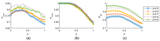
Figure 7.
The curve of recognition accuracy P with weight α at different β. (a) The accuracy of the test set; (b) The accuracy of the training set; and, (c) The accuracy of all images.
As can be seen from Figure 7a, when α is between 0.2 and 0.4, the proposed algorithm has the best recognition accuracy. Therefore, in subsequent experiments, α is 0.3 will be used to calculate .
Figure 8 shows the curve of overall recognition accuracy changing with the training images ratio β at different image size L × L. Figure 9 shows the accuracy of different models changing with β at L = 100. It can be seen from Figure 8 that the recognition accuracy of the test set is between 70% and 85%, the recognition accuracy of the training set is grater than 99%, and the total recognition accuracy is greater than 80%. The recognition accuracy generally increases as β increases. However, the number of images in the test set is too small when β is greater than 0.9, so the accuracy of the test set has a large deviation.
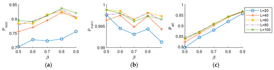
Figure 8.
The curve of overall accuracy changing with the training images ratio β at different image size. (a) The accuracy of the test set; (b) The accuracy of the training set; and, (c) The accuracy of all images.

Figure 9.
The accuracy of different models changing with the training images ratio β at L = 100. (a) The accuracy of the test set; (b) The accuracy of the training set; and, (c) The accuracy of all images.
Figure 10 and Figure 11 show the curve of the accuracy changing with the size of the image. Figure 10 shows the overall accuracy of all models. Figure 11 shows the respective accuracy for different models. As can be seen from the figures, when the image size L is as low as 20, the test accuracy rapidly decreases. When L is greater than 40, the accuracy increases slowly. Figure 10 shows that, when β is equal to 0.8, the accuracy reaches a maximum. Figure 9 and Figure 11 show that the mcar model has the highest accuracy and the fcarb model has the lowest accuracy. This experimental result shows that the proposed algorithm can be implemented at a lower image resolution, which can reduce the calculation time.
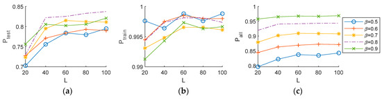
Figure 10.
The curve of the overall accuracy changing with the size of the image at different β. (a) The accuracy of the test set; (b) The accuracy of the training set; and, (c) The accuracy of all images.
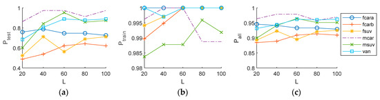
Figure 11.
The accuracy of different models changing with the size of the image at β = 0.8. (a) The accuracy of the test set; (b) The accuracy of the training set; and, (c) The accuracy of all images.
Figure 12 shows the correctly recognized and incorrectly recognized images of fcara and fcarb in one experiment. Figure 12a–d show the images of fcara. Figure 12e–h show the images of fcarb. As can be seen from the figures, the quality of the imaging results is uneven, some are good, some are poor. Figure 12b,f show the normal images. Figure 12c,g show the imaging distortion that might be caused by the position error of the radar. Figure 12d,h show incomplete imaging due to less than one circle of radar flying around the target.
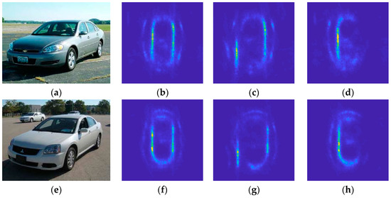
Figure 12.
The correctly recognized and incorrectly recognized images of fcara and fcarb in one experiment. (a) Visible image of fcara; (b) One of the correctly recognized fcara’s Wide-angle Synthetic Aperture Radar (WSAR) images; (c,d) One of the incorrectly recognized fcara’s WSAR images. (e) Visible image of fcarb; (f) One of the correctly recognized fcarb’s WSAR images; and, (g,h) One of the incorrectly recognized fcarb’s WSAR images.
5.2. Algorithm Comparison
At present, there are few researches regarding vehicle model recognition on the Gotcha dataset. Only a few papers address vehicle target recognition for wide-angle SAR. Dungan et al. proposed a vehicle discrimination algorithm based on point pattern matching, which achieved a recognition accuracy higher than 95% [27,29]. However, the data used by Dungan et al. is different from that in this paper. Dungan et al. used eight groups of altitude orbit data for the same vehicle at the same location for recognition. In this paper, 31 groups of altitude orbit data of different vehicles in different locations are used for recognition. The data that were used in this paper are much more difficult for recognition analysis.
Gianelli et al. proposed an imaging algorithm called data-adaptive Sparse Learning via Iterative Minimization (SLIM), and used the algorithm to achieve 90% recognition accuracy [32]. Gianelli et al. used basically the same dataset as in this paper, but they eliminated all of the flawed data and used only 540 images in total for the recognition experiment. In this paper, only the moving and changing image data of the vehicle is excluded, and a total of 660 images are used for the recognition experiment. No comparative experiment was conducted on the same dataset in this paper since it was impossible to know which image data were excluded from the Reference [32].
6. Conclusions
This paper presents a vehicle target recognition algorithm for WSAR. Based on the backprojection imaging algorithm, the modulus stretch transform function is added to the imaging process. The image after processing has thinner contour edges than that obtained from the traditional backprojection algorithm. After obtaining the contour image, the gravitational-based speckle reduction algorithm is used to obtain a clearer contour image. Subsequently, the image is rotated to obtain a standard orientation image. Hence, the image and projection feature set can be extracted from these processed images. Finally, the image and projection joint feature set matching algorithm is used to identify the vehicle model. The experiment analyzed the relationship between test accuracy, training accuracy and total accuracy with the variation of the parameter α, training images ratio and image size. The experiments show that the recognition accuracy is up to 85%, and the proposed algorithm can be implemented with low image resolution.
Author Contributions
Conceptualization, R.H.; Formal analysis, R.H. and J.M.; Funding acquisition, Z.P.; Investigation, R.H. and J.M.; Methodology, R.H.; Project administration, Z.P.; Software, R.H.; Supervision, Z.P.; Visualization, R.H.; Writing—original draft, R.H.; Writing—review and editing, Z.P.
Funding
This work is supported by National Natural Science Foundation of China (61571096, 61775030), Open Research Fund of Key Laboratory of Optical Engineering, Chinese Academy of Sciences (2017LBC003) and Sichuan Science and Technology Program (2019YJ0167).
Conflicts of Interest
The authors declare no conflict of interest.
References
- Peng, Z.; Zhang, J.; Meng, F.; Dai, J. Time-Frequency Analysis of SAR Image Based on Generalized S-Transform. In Proceedings of the 2009 International Conference on Measuring Technology and Mechatronics Automation (ICMTMA2009), Zhangjiajie, China, 11–12 April 2009; Volume 1, pp. 556–559. [Google Scholar]
- Peng, Z.; Wang, H.; Zhang, G.; Yang, S. Spotlight SAR images restoration based on tomography model. In Proceedings of the 2009 Asia-Pacific Conference on Synthetic Aperture Radar, APSAR 2009, Xi’an, China, 26–30 October 2009; pp. 1060–1063. [Google Scholar]
- Peng, Z.; Liu, S.; Tian, G.; Chen, Z.; Tao, T. Bridge detection and recognition in remote sensing SAR images using pulse coupled neural networks. In Proceedings of the 7th International Symposium on Neural Networks, ISNN 2010, Shanghai, China, 6–9 June 2010; Volume 67, pp. 311–320. [Google Scholar]
- Álvarez López, Y.; García Fernández, M.; Grau, R.; Las-Heras, F. A Synthetic Aperture Radar (SAR)-Based Technique for Microwave Imaging and Material Characterization. Electronics 2018, 7, 373. [Google Scholar] [CrossRef]
- Lao, G.; Yin, C.; Ye, W.; Sun, Y.; Li, G.; Han, L. An SAR-ISAR Hybrid Imaging Method for Ship Targets Based on FDE-AJTF Decomposition. Electronics 2018, 7, 46. [Google Scholar] [CrossRef]
- Qian, Y.; Zhu, D. High Resolution Imaging from Azimuth Missing SAR Raw Data via Segmented Recovery. Electronics 2019, 8, 336. [Google Scholar] [CrossRef]
- Qian, Y.; Zhu, D. Focusing of Ultrahigh Resolution Spaceborne Spotlight SAR on Curved Orbit. Electronics 2019, 8, 628. [Google Scholar] [CrossRef]
- Sun, D.; Xing, S.; Li, Y.; Pang, B.; Wang, X. Sub-Aperture Partitioning Method for Three-Dimensional Wide-Angle Synthetic Aperture Radar Imaging with Non-Uniform Sampling. Electronics 2019, 8, 629. [Google Scholar] [CrossRef]
- Burl, M.C.; Owirka, G.J.; Novak, L.M. Texture discrimination in synthetic aperture radar imagery. In Proceedings of the Asilomar Conference on Circuits, Systems & Computers, Pacific Grove, CA, USA, 30 October–1 November 1989; Volume 1, pp. 399–404. [Google Scholar]
- Mahalanobis, A.; Forman, A.V.; Bower, M.R.; Day, N.; Cherry, R.F. Quadratic distance classifier for multiclass SAR ATR using correlation filters. Ultrah. Resolut. Radar 1993, 1875, 84–95. [Google Scholar]
- Novak, L.M.; Owirka, G.J.; Netishen, C.M. Performance of a High-Resolution Polarimetric SAR Automatic Target Recognition System. Linc. Labor. J. 1993, 6, 11–24. [Google Scholar]
- Zhao, X.; Jiang, Y.; Stathaki, T. Automatic Target Recognition Strategy for Synthetic Aperture Radar Images Based on Combined Discrimination Trees. Comput. Intell. Neurosci. 2017, 2017, 1–18. [Google Scholar] [CrossRef]
- Ding, B.; Wen, G.; Zhong, J.; Ma, C.; Yang, X. A Robust Similarity Measure for Attributed Scattering Center Sets with Application to SAR ATR. Neurocomputing 2017, 219, 130–143. [Google Scholar] [CrossRef]
- Kechagias-Stamatis, O.; Aouf, N. Fusing Deep Learning and Sparse Coding for SAR ATR. IEEE Trans. Aerosp. Electron. Syst. 2018, 55, 785–797. [Google Scholar] [CrossRef]
- Franceschetti, G.; Lanari, R.; Pascazio, V.; Schirinzi, G. Wide angle SAR processors and their quality assessment. In Proceedings of the International Geoscience and Remote Sensing Symposium (IGARSS1991), Espoo, Finland, 3–6 June 1991; Volume 1, pp. 287–290. [Google Scholar]
- Franceschetti, G.; Lanari, R.; Pascazio, V.; Schirinzi, G. WASAR: A wide-angle SAR processor. IEE Proc. Part F Radar Signal Process. 1992, 139, 107–114. [Google Scholar] [CrossRef]
- Allen, M.R.; Phillips, S.A.; Sofianos, D.J. Wide-angle SAR-matched filter image formation for enhanced detection performance. In Proceedings of the Substance Identification Analytics, Innsbruck, Austria, 4–8 October 1993; pp. 381–387. [Google Scholar]
- Allen, M.R.; Hoff, L.E. Wide-angle wideband SAR matched filter image formation for enhanced detection performance. In Proceedings of the Algorithms for Synthetic Aperture Radar Imagery, Orlando, FL, USA, 5–8 April 1994; pp. 302–314. [Google Scholar]
- Mccorkle, J.W.; Rofheart, M. Order N2log(N) backprojector algorithm for focusing wide-angle wide-bandwidth arbitrary-motion synthetic aperture radar. In Proceedings of the International Society for Optics and Photonics, Orlando, FL, USA, 17 June 1996; Volume 2747, pp. 25–36. [Google Scholar]
- Trintinalia, L.C.; Bhalla, R.; Ling, H. Scattering center parameterization of wide-angle backscattered data using adaptive Gaussian representation. IEEE Trans. Antennas Propag. 1997, 45, 1664–1668. [Google Scholar] [CrossRef]
- Ertin, E.; Potter, L.C.; Mccorkle, J. Multichannel imaging for wide band wide angle polarimetric synthetic aperture radar. In Proceedings of the Algorithms for Synthetic Aperture Radar Imagery V, Orlando, FL, USA, 14–17 April 1998; Volume 3370, pp. 41–51. [Google Scholar]
- Guarnieri, A.M.; D’aria, D. Wide-angle azimuth antenna pattern estimation in SAR images. In Proceedings of the International Geoscience and Remote Sensing Symposium, Toulouse, France, 21–25 July 2003; pp. 3105–3107. [Google Scholar]
- Yocky, D.A.; Jakowatz, J.; Charles, V. Automated wide-angle SAR stereo height extraction in rugged terrain using shift-scaling correlation. In Proceeding of the Applications of Digital Image Processing XXVI, San Diego, CA, USA, 5–8 August 2003; Volume 5203, pp. 10–20. [Google Scholar]
- He, S.; Zhou, J.; Zhao, H.; Fu, Q. Resolution analysis for wide angle SAR imaging. In Proceedings of the 2007 1st Asian and Pacific Conference on Synthetic Aperture Radar, Huangshan, China, 5–9 November 2007; pp. 19–22. [Google Scholar]
- Moses, R.L.; Lee, P.C.; Cetin, M. Wide angle SAR imaging. In Proceedings of the Algorithms for Synthetic Aperture Radar Imagery XI, Orlando, FL, USA, 12–15 April 2004; Volume 5427, pp. 164–175. [Google Scholar]
- Casteel, J.C.H.; Gorham, L.A.; Minardi, M.J.; Scarborough, S.M.; Naidu, K.D.; Majumder, U.K. A challenge problem for 2D/3D imaging of targets from a volumetric data set in an urban environment. In Proceedings of Algorithms for Synthetic Aperture Radar Imagery XIV; International Society for Optics and Photonics: Orlando, FL, USA, 2007. [Google Scholar]
- Dungan, K.E.; Potter, L.C.; Blackaby, J.; Nehrbass, J. Discrimination of civilian vehicles using wide-angle SAR. In Proceedings of the SPIE Defense and Security Symposium, Orlando, FL, USA, 17–18 March 2008. [Google Scholar]
- Dungan, K.E.; Potter, L.C. Effects of polarization on wide-angle SAR classification performance. In Proceedings of the 2010 IEEE National Aerospace Electronics Conference, Fairborn, OH, USA, 14–16 July 2010; pp. 50–53. [Google Scholar]
- Dungan, K.E.; Potter, L.C. Classifying vehicles in wide-angle radar using pyramid match hashing. IEEE J. Sel. Top. Signal Process. 2011, 5, 577–591. [Google Scholar] [CrossRef]
- Dungan, K.E.; Ash, J.N.; Nehrbass, J.W.; Parker, J.T.; Gorham, L.A.; Scarborough, S.M. Wide angle SAR data for target discrimination research. In Proceedings of the SPIE Defense, Security, and Sensing, Baltimore, MD, USA, 25–26 April 2012. [Google Scholar]
- Ertin, E. Manifold learning methods for wide-angle SAR ATR. In Proceedings of the 2013 International Conference on Radar—Beyond Orthodoxy: New Paradigms in Radar, Adelaide, Australia, 9–12 September 2013; pp. 500–504. [Google Scholar]
- Gianelli, C.D.; Xu, L. Focusing, imaging, and atr for the gotcha 2008 wide angle sar collection. In Proceedings of the SPIE Defense, Security, and Sensing, Baltimore, MD, USA, 1–2 May 2013. [Google Scholar]
- Saville, M.A.; Jackson, J.A.; Fuller, D.F. Rethinking vehicle classification with wide-angle polarimetric SAR. Aerosp. Electron. Syst. Mag. 2014, 29, 41–49. [Google Scholar] [CrossRef]
- Li, Y.; Jin, Y. Target decomposition and recognition from wide-angle SAR imaging based on a Gaussian amplitude-phase model. Sci. China Inf. Sci. 2017, 60, 062305. [Google Scholar] [CrossRef]
- Hu, R.; Peng, Z.; Zheng, K. Modulus Stretch-Based Circular SAR Imaging with Contour Thinning. Appl. Sci. 2019, 9, 2728. [Google Scholar] [CrossRef]
- Wang, X.; Peng, Z.; Zhang, P.; He, Y. Infrared Small Target Detection via Nonnegativity-Constrained Variational Mode Decomposition. IEEE Geosci. Remote Sens. Lett. 2017, 14, 1700–1704. [Google Scholar] [CrossRef]
- Liu, X.; Chen, Y.; Peng, Z.; Wu, J.; Wang, Z. Infrared Image Super-Resolution Reconstruction Based on Quaternion Fractional Order Total Variation with Lp Quasinorm. Appl. Sci. 2018, 8, 1864. [Google Scholar] [CrossRef]
- Zhang, T.; Wu, H.; Liu, Y.; Peng, L.; Yang, C.; Peng, Z. Infrared small target detection based on non-convex optimization with Lp-norm constraint. Remote Sens. 2019, 11, 559. [Google Scholar] [CrossRef]
- Peng, L.; Zhang, T.; Liu, Y.; Li, M.; Peng, Z. Infrared Dim Target Detection Using Shearlet’s Kurtosis Maximization under Non-Uniform Background. Symmetry 2019, 11, 723. [Google Scholar] [CrossRef]
- Li, X.; Wang, J.; Li, M.; Peng, Z.; Liu, X. Investigating Detectability of Infrared Radiation Based on Image Evaluation for Engine Flame. Entropy 2019, 21, 946. [Google Scholar] [CrossRef]
- Tian, S.; Sun, G.; Wang, C.; Zhang, H. A Ship Detection Method in SAR Image Based on Gravity Enhancemen. J. Remote Sens. 2007, 11, 452–459. (In Chinese) [Google Scholar]
- Kong, F. Maritime Traffic Monitoring and Analysis System Based on Satellite Remote Sensing. Master Thesis, Dalian Maritime University, Dalian, China, 2009. (In Chinese). [Google Scholar]
- Ballard, D.H. Generalizing the Hough transform to detect arbitrary shapes. Pattern Recognit. 1981, 13, 111–122. [Google Scholar] [CrossRef]


© 2019 by the authors. Licensee MDPI, Basel, Switzerland. This article is an open access article distributed under the terms and conditions of the Creative Commons Attribution (CC BY) license (http://creativecommons.org/licenses/by/4.0/).