Abstract
In this paper, path loss and time-dispersion results of the propagation channel in a typical office environment are reported. The results were derived from a channel measurement campaign carried out at 26 GHz in line-of-sight (LOS) and obstructed-LOS (OLOS) conditions. The parameters of both the floating-intercept (FI) and close-in (CI) free space reference distance path loss models were derived using the minimum-mean-squared-error (MMSE). The time-dispersion characteristics of the propagation channel were analyzed through the root-mean-squared (rms) delay-spread and the coherence bandwidth. The results reported here provide better knowledge of the propagation channel features and can be also used to design and evaluate the performance of the next fifth-generation (5G) networks in indoor office environments at the potential 26 GHz frequency band.
Keywords:
5G; mmWave; path loss; time-dispersion; delay-spread; coherence bandwidth; channel measurements 1. Introduction
Some of the main objectives proposed in the deployment of the future fifth-generation (5G) systems are the increase in the data rate and capacity, greater than 100 Mbps, with peak data rates up to 10 Gbps, ultra-reliable and low-latency communications, and communications in high user density scenarios [1,2]. The first 5G deployments, at least at the European level, will be carried out in the harmonized frequency bands below 1 GHz, in particular the 700 MHz band, corresponding to the second digital dividend, together with the 3.4–3.8 GHz frequency band [3]. However, the high transmission rates expected in 5G can only be achieved using the spectrum at frequencies above 24 GHz, where it is possible to use bandwidths of the order of hundreds of megahertz [2]. At the last World Radiocommunication Conference (WRC) of the International Telecommunication Union (ITU), held in 2015 (WRC-15), the potential bands to locate future 5G systems, on a primary basis, above 24 GHz are: 24.25–27.5 GHz, 31.8–33.4 GHz, and 37–40.5 GHz, [4]. Although the final decision will be conditioned in part by the industry, the potential for global harmonization, and research works, there is some consensus to deploy the 5G systems in the 26 GHz frequency band. In fact, the Radio Spectrum Policy Group (RSPG) has recommended the 24.25–27.5 GHz band for the 5G deployments in Europe.
Many measurement campaigns in both indoor and outdoor environments have been conducted at some typical millimeter wave (mmWave) bands (although the mmWave band strictly corresponds to frequencies between 30 and 300 GHz, it is common in the literature to also consider frequencies above 10 GHz), in particular at 11, 15, 28, 38, 60, and 73 GHz [5,6,7,8,9]. Nevertheless, little attention has been devoted to the 26 GHz band. Although the propagation characteristics measured at 28 GHz could be extrapolated to the 26 GHz frequency band, specific channel measurements are necessary for better knowledge of the propagation channel. In this sense, a contribution to the path loss and time-dispersion characterization, in terms of the delay-spread and the coherence bandwidth, is performed in this paper. The study is based on a channel measurement campaign at 26 GHz carried out in an indoor office environment. The measurements were collected under line-of-sight (LOS) and obstructed-LOS (OLOS) conditions with a channel sounder implemented in the frequency domain using a vector network analyzer (VNA) and a broadband radio over fiber (RoF) link to increase the dynamic range in the measurement and allowing us to use omnidirectional antennas at the transmitter (Tx) and the receiver (Rx).
2. Channel Measurements
2.1. Propagation Environment
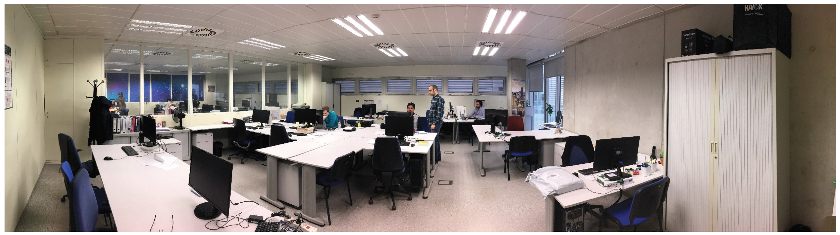
The channel measurements were carried out in an office environment, characterized by the presence of desks, with PC monitors, chairs, and some steel storage cabinets, among other typical objects in these environments. The office was in a modern building construction with large exterior glass windows, where the ceiling and the floor were built of reinforced concrete over steel plates with wood and plasterboard paneled walls. Figure 1 shows a panoramic view of the office. The propagation environment consisted of a 9.68 m by 6.93 m room with a height of 2.63 m.
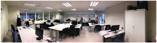
Figure 1.
Panoramic view of the propagation environment.
2.2. Measurement Setup and Procedure
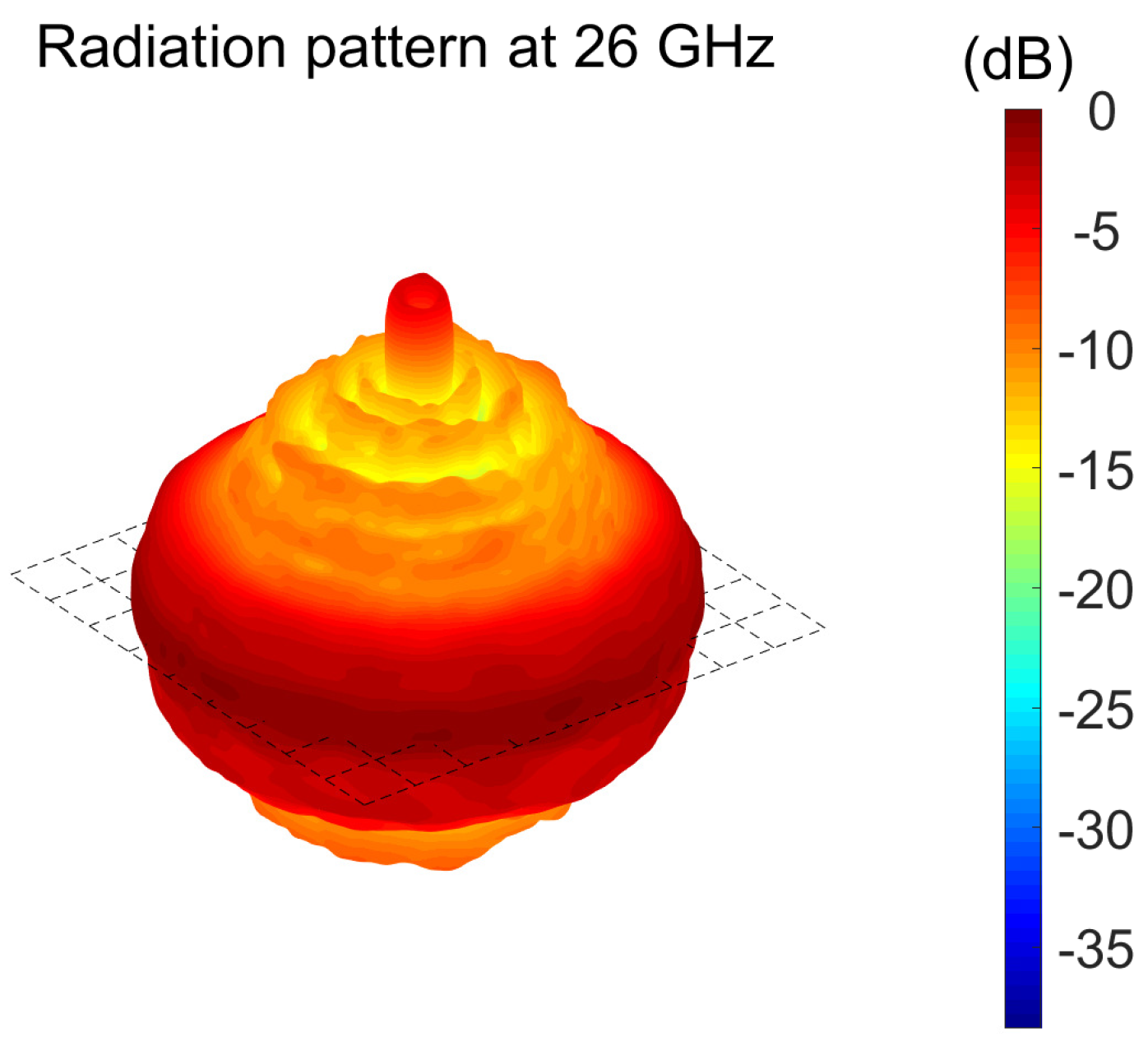
A channel sounder was implemented in the frequency domain to measure the complex channel transfer function (CTF), denoted as . The channel sounder was based on the Keysight N5227A VNA. The QOM-SL-0.8-40-K-SG-L ultra-wideband antennas, developed by Steatite Ltd company, were used at the Tx and Rx sides. These antennas operate from 800 MHz to 40 GHz, have an omnidirectional radiation pattern in the azimuth plane (horizontal plane), and linear polarization. Figure 2 shows the three-dimensional (3D) radiation pattern of the antennas measured in our anechoic chamber. The 3 dB beamwidth of the antennas in the elevation plane, known as half power beamwidth (HPBW), was in the order of 35 at 26 GHz.

Figure 2.
3D radiation pattern of the antenna at 26 GHz.
The Tx antenna was connected to the VNA through an amplified broadband RoF link, the Optica OTS-2 model developed by Emcore (from 1 to 40 GHz, with 35 dB of gain). This RoF link avoided the high losses of cables at mmWave frequencies, thus increasing the dynamic range in the measurement and allowing us to use omnidirectional antennas due to the fact that significant features of the propagation channel, such as time-dispersion, could be affected by the use of directional antennas [10].
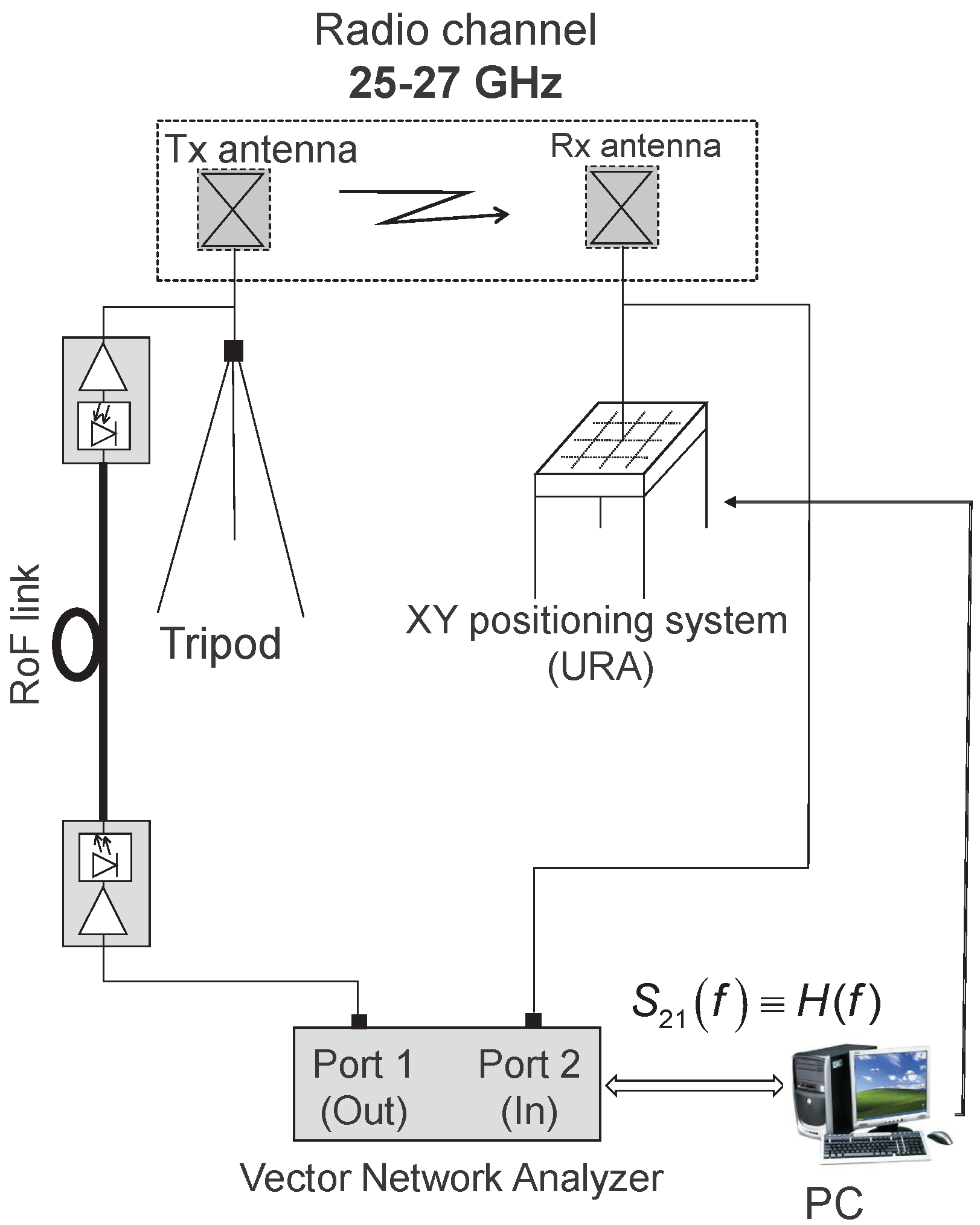
The Rx antenna was located in a XY positioning system, implementing a uniform rectangular array (URA). The inter-element separation of the URA was 3.04 mm. This separation was about at 26 GHz, covering the Rx antenna with a local area around in order to take into account small-scale fading effects. Both the VNA and the XY positioning system were controlled by a personal computer. The scattering parameter, equivalent to [11], was measured from 25 to 27 GHz, i.e., a channel bandwidth (SPAN in the VNA) of 2 GHz was employed with 26 GHz as a central frequency. Notice that a VNA measures the scattering parameters of a device under test (DUT). In this case, the DUT was the wireless channel, where the scattering parameter was the CTF at the frequency that was used to excite the channel. By having the excitation signal sweep through the frequency band of interest, i.e., the SPAN, a sampled version of the CTF was measured. The radiofrequency signal level at the VNA was dBm to not saturate the amplifier at the input of the electro-optical converter in the RoF link. Before the measurements, the channel sounder was calibrated carefully. A response calibration process was performed, moving the time reference points from the VNA port to the calibration points. Thus, the measured CTF took into account the joint response of the propagation channel and the Tx and Rx antennas, also known in the literature as the radio channel [12]. A schematic diagram of the channel sounder is shown in Figure 3.
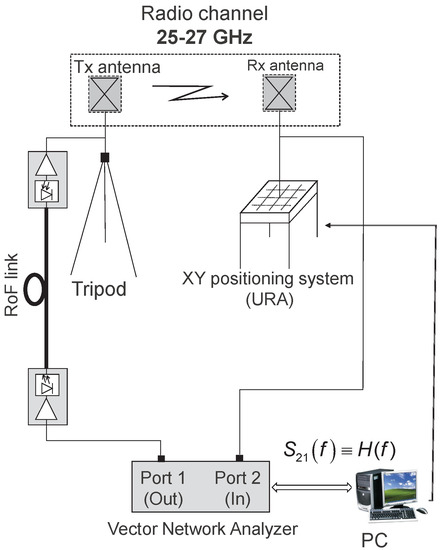
Figure 3.
Schematic diagram of the channel sounder.
A total of frequency points was measured over the 2 GHz bandwidth. Thus, the frequency resolution was about MHz (), which corresponded to a maximum unambiguous excess delay estimated as of 546 ns. This maximum unambiguous excess delay was equivalent to a maximum observable distance calculated as , with the speed of light, of about 164 m. Notice that the maximum observable distance was larger than the office dimensions, ensuring that all multipath contributions were captured. The bandwidth of the intermediate frequency (IF) filter at the VNA, denoted by , was set to 100 Hz. This value of was a trade-off between acquisition time and dynamic range in the measurement. Thus, low values of reduced the noise floor, increasing the dynamic range in the measurement. Nevertheless, low values of increased the acquisition time. As a reference, in [7], the authors used 500 Hz in indoor office channel measurements at mmWave frequencies. Table 1 summarizes the measurement system parameters.

Table 1.
Measurement system parameters.
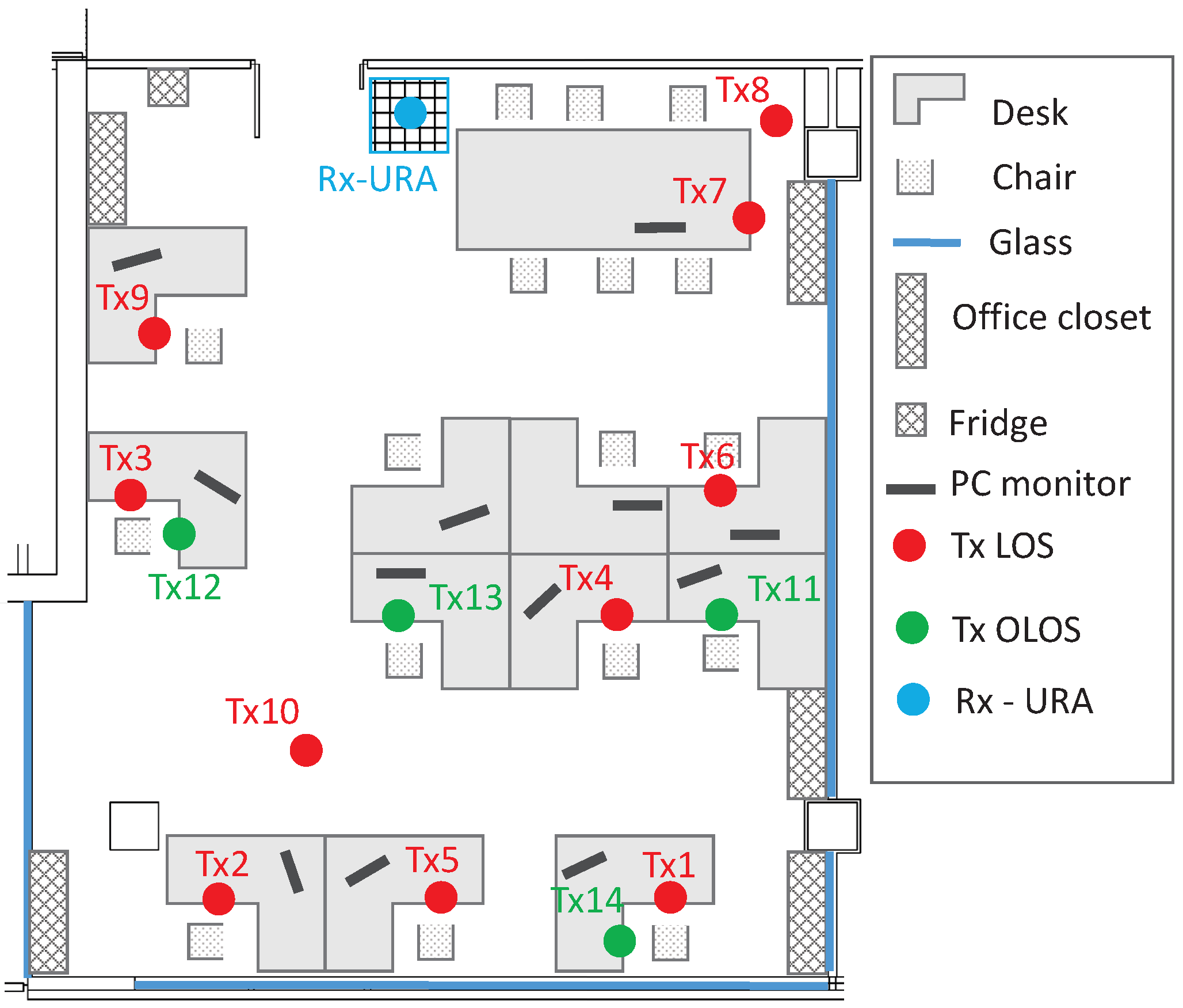
During the measurements, the Tx antenna was located manually in different locations of the office, imitating the position of user equipment (UE). The Rx subsystem remained fixed in the same position, close to the wall, imitating an access point (AP) that served the users inside the office. The Rx antenna height was 1.62 m with respect to the floor. With the VNA configuration parameters, i.e., and , the acquisition time to capture the CTF in the 144 () positions of the Rx antenna in the URA was about 2 h. To guarantee stationary channel conditions (due to the frequency sweep time to measure the scattering parameter, the acquisition of the channel measurements required stationary channel conditions), the measurements were collected at night, thus avoiding the presence of people, not only in the measurement room, but also in adjoining areas. Figure 4 shows the top view of the propagation environment, together with the Rx-URA position and the Tx antenna locations. The channel measurements were performed in LOS and OLOS conditions, defining two scenarios:
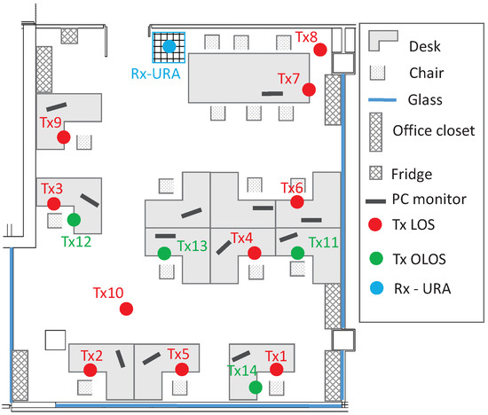
Figure 4.
Top view of the propagation environment. The Rx-URA and the Tx antenna locations are indicated.
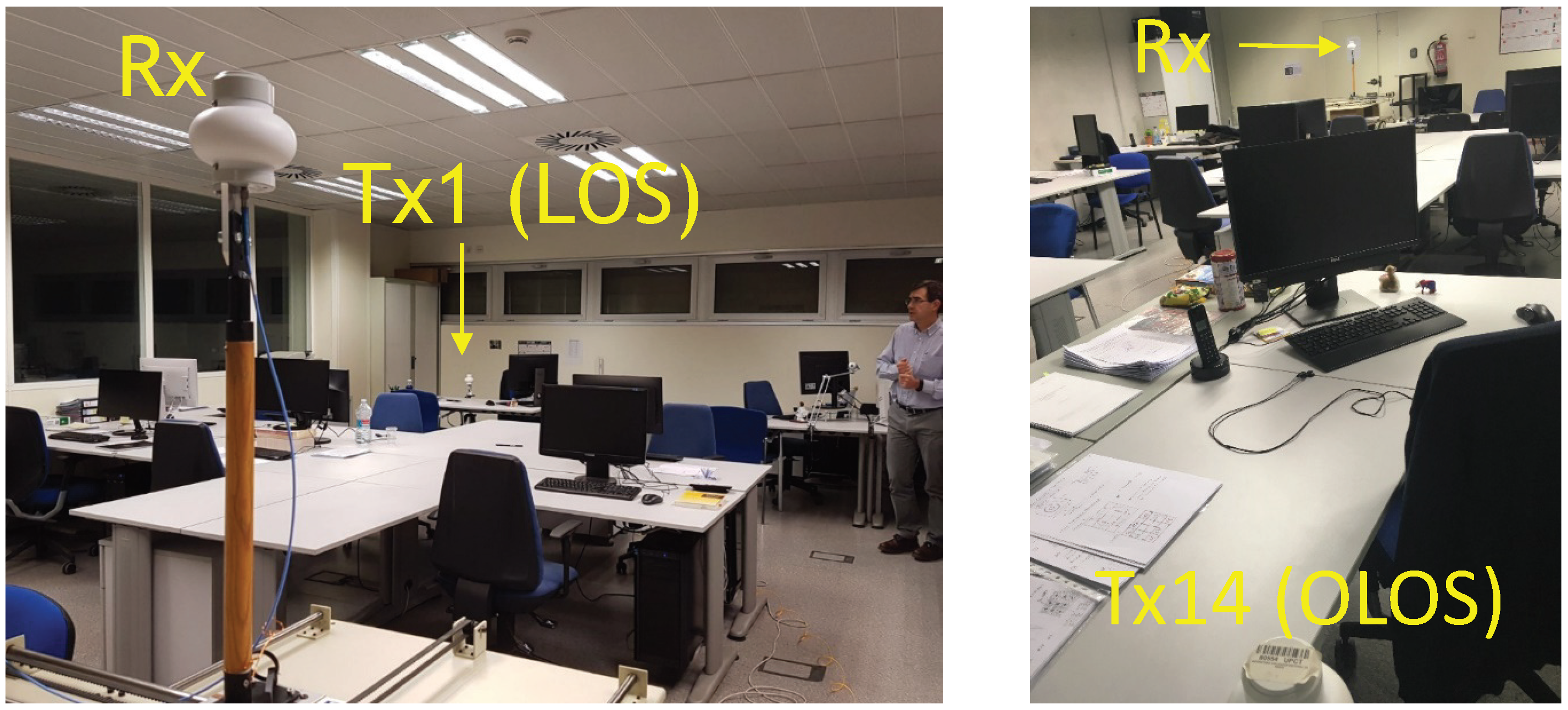
- Scenario LOS: The Tx antenna was located at a height of 0.90 m above the floor level, imitating the position of a UE (e.g., a laptop, tablet, or mobile phone) that was on the desk. A total of 10 Tx locations (Tx1–Tx10) was considered in the measurements. Figure 5 (left) shows a view of the Rx-URA and the Tx antenna for the Tx1 position.
 Figure 5. View of the Rx antenna and the Tx antenna in positions Tx1 in LOS (left) and Tx14 in OLOS (right).
 - Scenario OLOS: The Tx antenna was also located at a height of 0.90 m above the floor and close to the desk, but in OLOS propagation conditions due to the blockage of the direct component by the computer monitors on the desks. The measurements were taken in 4 Tx locations (Tx11-Tx14). Figure 5 (right) shows a view of the Rx-URA and the Tx antenna for the Tx14 position.
3. Measurement Results
3.1. Path Loss Results
For each position of the URA, the path loss between the Tx and Rx antennas can be derived by averaging the CTF in frequency and taking into account the gain of both antennas in the direct path [13]. Thus, the path loss in logarithmic units, PL, can be derived as (see Appendix A):
where d refers to the separation distance between the Tx antenna and the center of the URA for each Tx location, indicated as Tx-Rx distance; is the nth frequency sample; and and are the gain of the Tx and Rx antennas, respectively, in the direction defined by the direct path contribution. The term takes into account the mismatch of the antennas, and it is calculated by:
and being the scattering parameter of the Tx and Rx antennas, respectively.
The measured path loss (cross marker) for each Rx antenna position in the URA in terms of the Tx-Rx distance is shown in Figure 6. Both LOS and OLOS propagation conditions were considered. It is worth noting that the spread values of the path loss along the URA due to the short-term fading was less than 2.5 dB, being less in LOS than in OLOS conditions. It can be observed that the spread values of the path loss did not exhibit any correlation with the Tx-Rx distance. The mean value of the path loss (square marker) for each Tx location is also depicted in Figure 6.
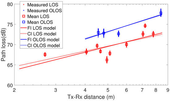
Figure 6.
Path loss in terms of the Tx-Rx distance. Measured data, measured mean values, and estimated values from the CI and FI models, in both LOS and OLOS conditions.
The floating-intercept (FI) path loss model has been widely used to describe the behavior of the path loss in terms of the Tx-Rx distance in the microwave frequency band, particularly at the sub-6 GHz band and more recently in mmWave frequencies [5,14], being one of the propagation models adopted in channel standardizations, e.g., the WINNERII Project and 3GPP channel models [15,16]. From the FI model, the path loss is given by:
being the floating-intercept parameter (an offset term); the path loss exponent, related to both the environment and propagation conditions; and a zero mean Gaussian random variable, in logarithmic units, with standard deviation , which describes the large-scale signal fluctuations about the mean path loss over distance, also known in the literature as the shadow factor (SF). The FI model has a mathematical curve fitting approach over the measured path loss set without any physical anchor.
On the other hand, the close-in (CI) free space reference distance path loss model is also adopted in many studies related to mmWave propagation [5,8]. In the CI model, the path loss is given by:
where is the free space path loss for a Tx-Rx distance equal to 1 m, with the speed of light; n is the path loss exponent; and is the SF term. Note that the CI model has certain physical support in the sense that there is an intrinsic frequency dependence of the path loss included in the 1 m FSPL term. Taking into account that is equal to 60.74 dB at 26 GHz, (4) can be rewritten as:
The path loss fitting results for the FI and CI models are also depicted in Figure 6. Both models exhibit a good fit and predict similar path loss values for the Tx-Rx distance considered, particularly in OLOS conditions. It is worth noting that the maximum path loss difference between LOS and OLOS conditions was about 5 dB, increasing with the Tx-Rx distance. Table 2 and Table 3 summarize the mean value and their 95% confidence interval of the FI and CI model parameters. These parameters were derived from the measured path loss using the minimum-mean-squared-error (MMSE) approach.
Table 2.
FI path loss model parameters.
Table 3.
CI path loss model parameters.
For the FI model, had a mean value equal to 1.46, with 1.39–1.53 the 95% confidence interval, in LOS conditions. In OLOS conditions, had a mean value equal to 1.88, with 1.80–1.95 the 95% confidence interval. For the CI model, had a mean value equal to 1.27 and 1.79 for LOS and OLOS conditions, respectively. The 95% confidence intervals were narrower for the CI model. In both models, the SF had a similar value, being lower in OLOS conditions.
The values of the path loss exponent derived in this study were lower than the values reported in [8], where path loss exponents in the order or 2.0 and 2.2 were measured at 28 GHz in LOS and non-LOS (NLOS) conditions, respectively, for the FI model. Nevertheless, higher values have been reported for the CI model, where the path loss exponents equal to 1.45 and 2.18 have been measured in LOS and NLOS conditions, respectively. These differences can be explained because the frequencies are slightly different and, of course, due to both the particular characteristics of the environments and propagation conditions. It is worth noting that in our OLOS measurements, only a few MPCs were blocked by the PC monitors, whereas in NLOS conditions, the Tx and Rx were usually separated by different obstructions, and in many cases, the Tx and Rx were not located in the same room. Despite this, our results were more in line with those published by Rappaport et al. in [5,17] for indoor environments at 28 GHz in LOS conditions, where exponents equal to 1.2 and 1.1 were derived for the FI and CI models, respectively, considering omnidirectional path loss modeling (Rappaport et al. used a sliding correlation channel sounder, synthesizing an omnidirectional path loss model from directional measurements). Furthermore, the SF derived was 1.8 dB in both the FI and CI model, a value very close to that obtained by us for the CI model (1.75 dB).
3.2. Time-Dispersion Results
In wideband systems, the multipath propagation causes the arriving signal at the Rx to have a longer duration than the transmitted signal. This effect is the well-known time-dispersion of a wireless channel [11]. In the frequency domain, the time-dispersion can be interpreted as frequency selectivity, i.e., the CTF varies over the bandwidth of interest. The knowledge of the time-dispersion of a wireless channel is vital in the design of wireless systems, for example adopting efficient equalizer structures or defining the optimal multicarrier separation in digital modulations and diversity schemes. In this section, the time-dispersion of the propagation environment is analyzed in both the delay (time) and frequency domains.
3.2.1. Root-Mean-Squared Delay-Spread
The root-mean-squared (rms) delay-spread, denoted by , is the most relevant parameter to describe the time-dispersion of a wireless channel in the delay domain. corresponds to the second-order central moment of the power delay profile (PDP), and it is derived as [18]:
where refers to the nth delay bin in the PDP. Assuming ergodicity [11], the PDP can be estimated averaging the channel impulse response (CIR), denoted by , over all positions of the Rx antenna in the URA:
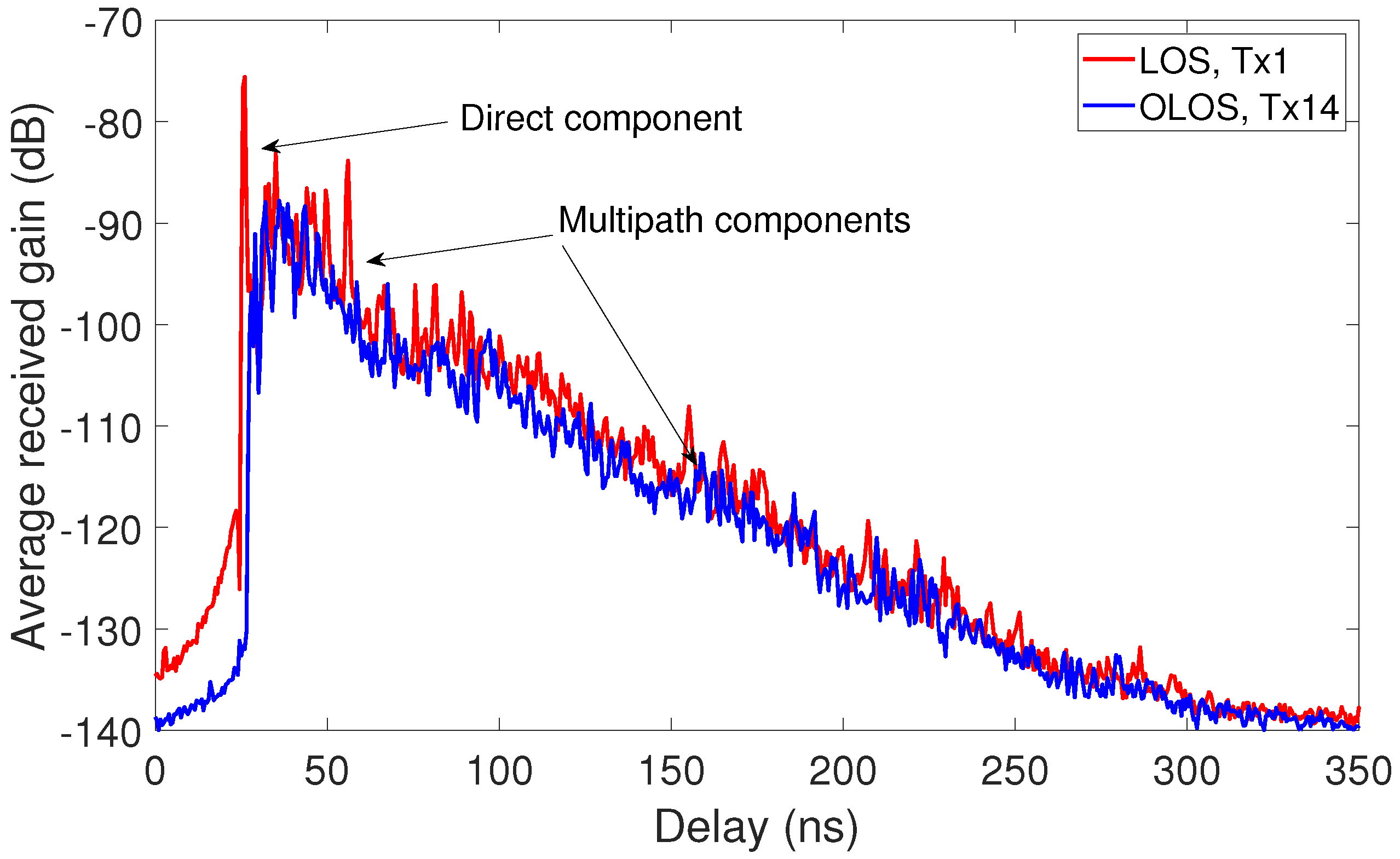
The CIR is obtained as the inverse Fourier transform of . As an example, Figure 7 shows the PDP measured in the Tx1 (LOS condition) and Tx14 (OLOS condition) positions. The differences between LOS and OLOS conditions for low delays can be observed, where the PC monitors blocked the first MPCs, in this case with excess delays around 50 ns.
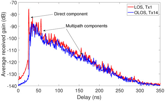
Figure 7.
PDP measured in Tx1 and Tx14 positions with LOS and OLOS propagation conditions, respectively.
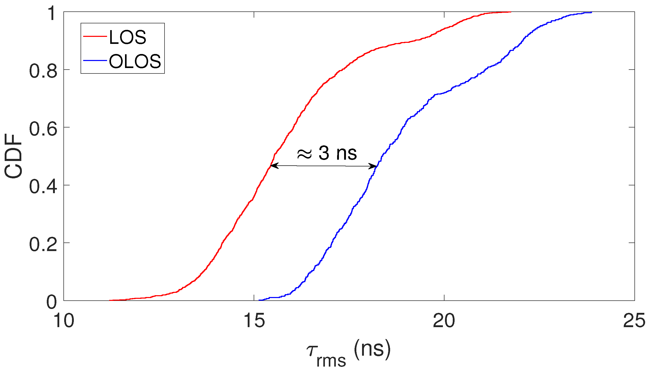
The cumulative distribution function (CDF) of for the LOS and OLOS scenarios is shown in Figure 8. A threshold of 30 dB and a Hamming windowing method were considered in the derivation of . Both curves exhibited a similar trend, with a separation of the order of 3 ns around the mean values. The results showed that the time-dispersion was slightly higher in the OLOS scenario. The minimum, mean, maximum, and standard deviation (STD) values of are summarized in Table 4. For the LOS scenario, ranged from 11.21 to 21.74 ns, with a mean value equal to 15.88 ns; whereas in the OLOS scenario, the values were higher, with ranging from 15.13 to 27.87 ns, with a mean value equal to 18.87 ns, 3 ns more than in the LOS scenario. Nevertheless, the STD of was very similar in both scenarios, in the order of 2 ns. It is worth noting that the values of derived here were higher than those published in [7] for an office environment, where values of 8 and 10 ns were reported at 28 and 38 GHz, respectively, in LOS conditions.
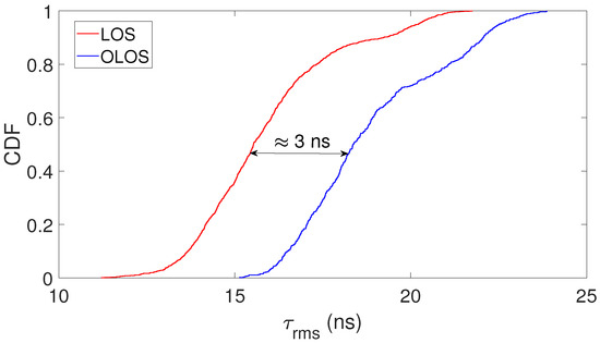
Figure 8.
CDF of for the LOS and OLOS scenarios.
Table 4.
Minimum, mean, maximum, and STD values of (in ns) and (in MHz).
3.2.2. Coherence Bandwidth
The frequency selectivity of a wideband wireless channel can be described through the frequency correlation function, denoted by , calculated as the Fourier transform of the PDP [18]:
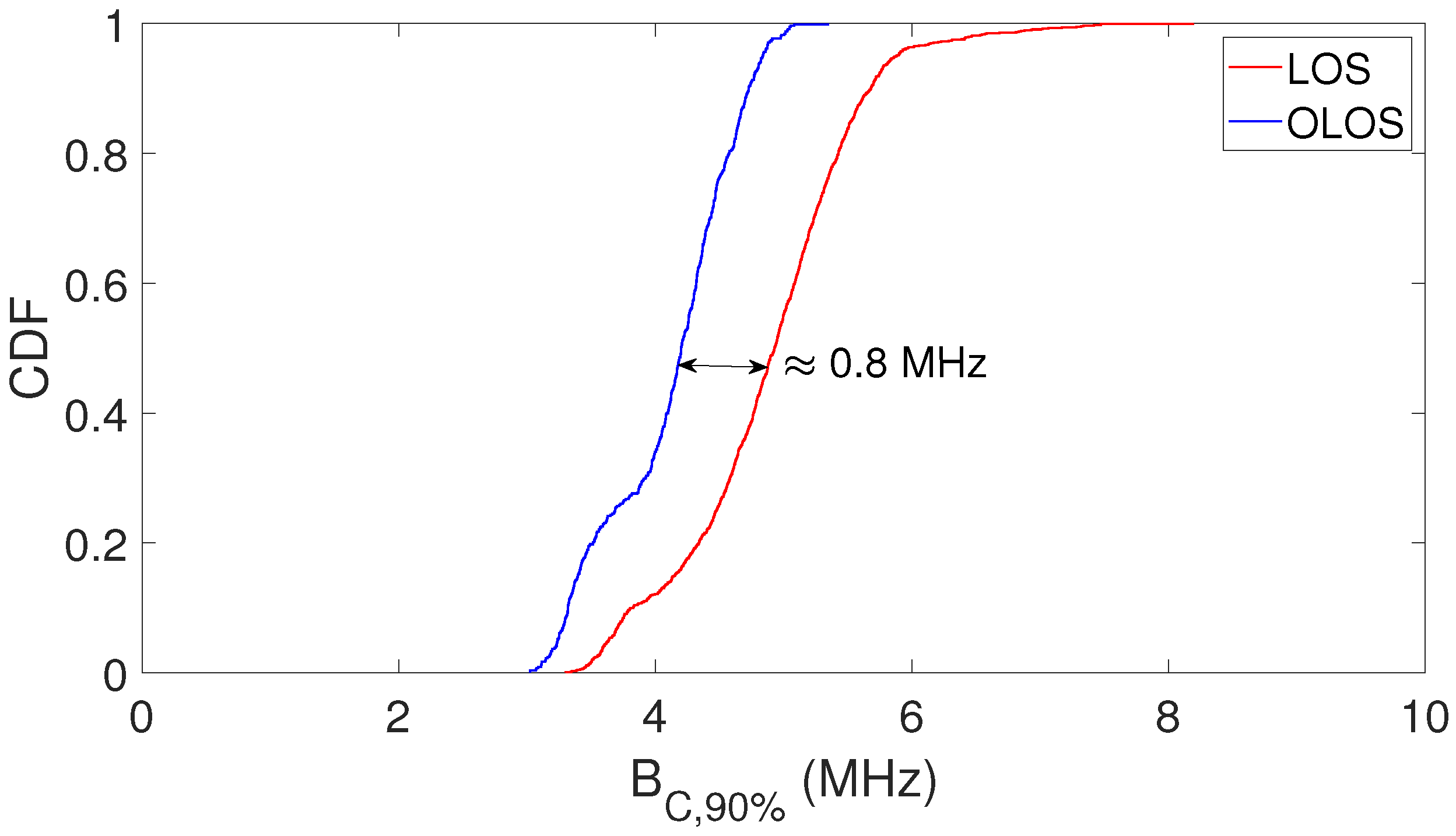
From (9), the coherence bandwidth can be defined as the smallest value of for which equals a certain correlation coefficient, typically 0.9 (or 90%). Figure 9 shows the CDF of the 90% coherence bandwidth, denoted as . The minimum, mean, maximum, and standard deviation (STD) values of are summarized in Table 4. The values of the coherence bandwidth had a higher dispersion in LOS conditions, where ranged from 3.30 to 8.19 MHz, with a mean value equal to 4.88 MHz. In OLOS conditions, the maximum value of was in the order of 5 MHz. Nevertheless, the difference between the mean value in LOS and OLOS conditions was not significantly high, about 0.8 MHz.

Figure 9.
CDF of for the LOS and OLOS scenarios.
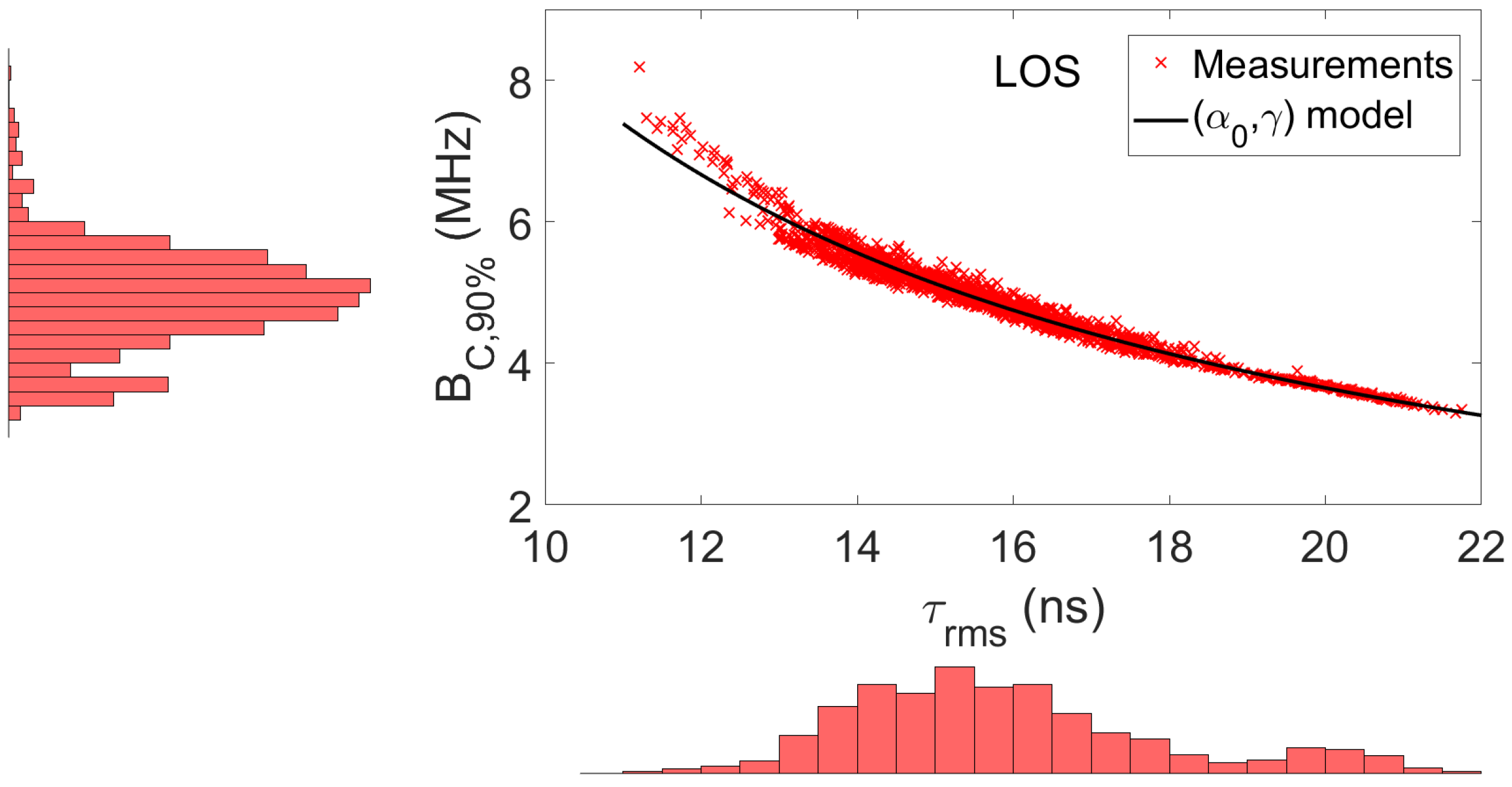
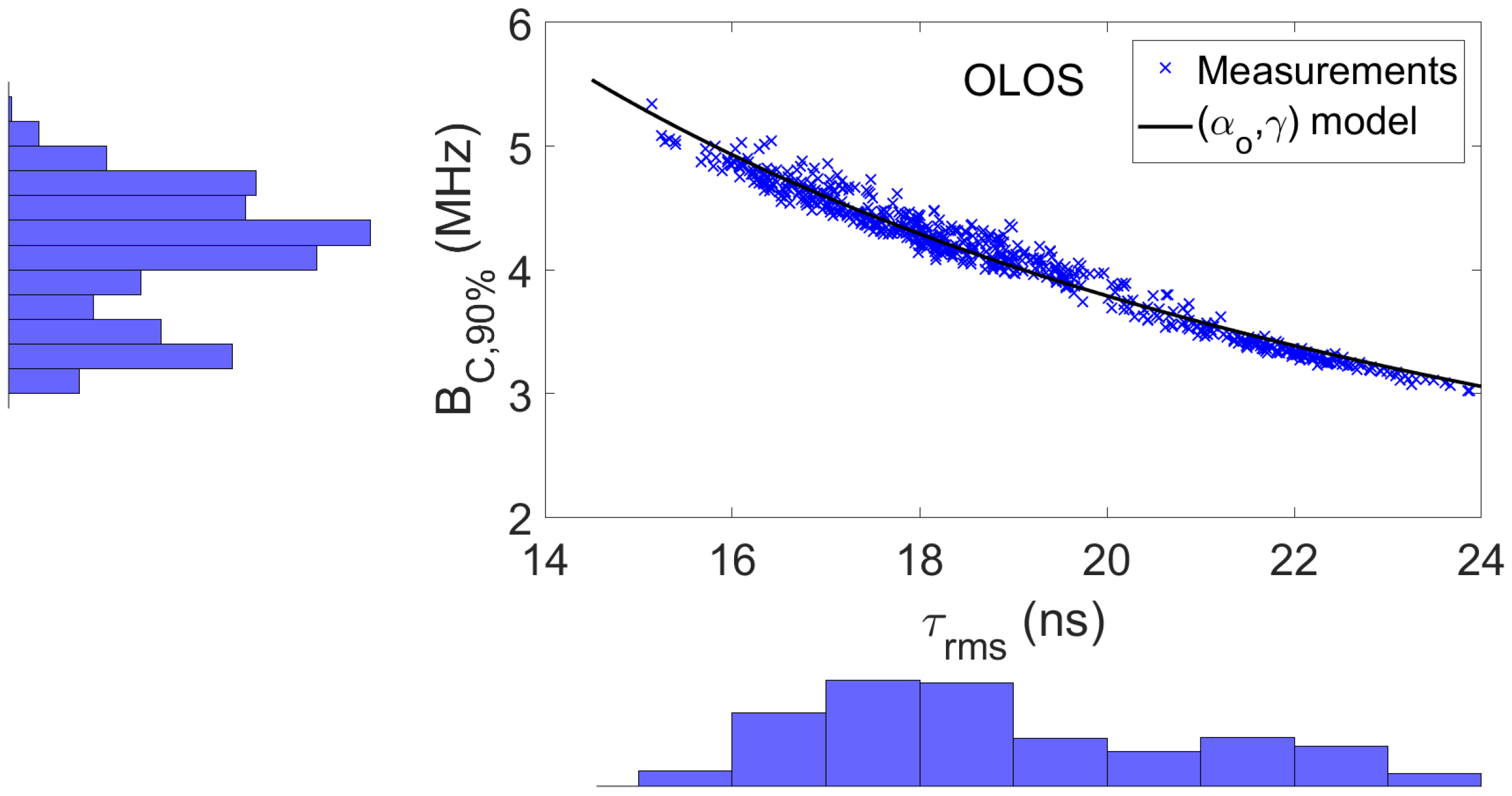
In order to investigate the relationship between the time-dispersion in the delay and frequency domains, Figure 10 and Figure 11 show the scatter plot of the 90% coherence bandwidth versus . The black line in both figures establishes a relationship between and in the form:

Figure 10.
Scatter plot of the 90% coherence bandwidth versus in LOS conditions.
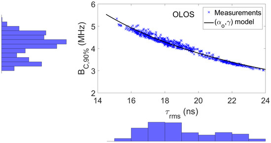
Figure 11.
Scatter plot of the 90% coherence bandwidth versus in OLOS conditions.
Equation (10) is an empirical expression, first proposed in [19], to try to model the relationship between the coherence bandwidth and . The relationship between the PDP and the autocorrelation function through the Fourier transform makes the consistent assumption that the relationship between and must be inverse. In fact, prior to the model given by (10), simpler expressions have been proposed, defined by a single parameter, , considering in (10) [20]. The variability of the PDP in different locations, even in the same propagation environment, makes it advisable to adopt a two-parameter model as proposed in [19]. Table 5 summarizes the values of and that appear in (10) using the MMSE approach. The 95% confidence intervals are also included in the table. Notice that the mean value of was the same in both scenarios; only differences appear in the values that define the 95% confidence interval.
Table 5.
Values of and (in ns).
4. Conclusions
In this paper, the path loss and time-dispersion characteristics of the propagation channel in a typical office environment were analyzed from a channel measurement campaign carried out at 26 GHz. The channel measurements were collected under LOS and OLOS conditions. The parameters of the FI and CI path loss models and their 95% confidence interval were derived from the measurements using the MMSE approach. Mean path loss exponents equal to 1.46 and 1.88 were derived for the FI model in LOS and OLOS, respectively. For the CI model, the mean path loss exponent was equal to 1.27 and 1.79 in LOS and OLOS, respectively. The results showed a maximum path loss difference between LOS and OLOS in the order of 5 dB.
The time-dispersion due to the multipath propagation was analyzed through the delay-spread and the coherence bandwidth. Mean values of equal to 15.88 and 18.87 ns were derived in LOS and OLOS, respectively; and mean values of the 90% coherence bandwidth equal to 4.88 and 4.11 were derived in LOS and OLOS, respectively. Furthermore, the correlation between the coherence bandwidth and the delay-spread was investigated, observing an inverse relationship between them.
The results reported in this contribution enable better knowledge of the propagation characteristics in office environments at 26 GHz and can be used to improve the design and evaluate the performance of the future 5G networks in these scenarios.
Author Contributions
Conceptualization, L.R., R.P.T., V.M.R.P. and J.-M.M.-G.-P.; data curation, L.R., V.M.R.P., J.R. and J.-M.M.-G.-P.; formal analysis, L.R., R.P.T., V.M.R.P. and J.-M.M.-G.-P.; funding acquisition, L.R., R.P.T., V.M.R.P. and J.-M.M.-G.-P.; investigation, L.R., R.P.T., V.M.R.P., J.R.P., J.R. and J.-M.M.-G.-P.; methodology, L.R., V.M.R.P. and R.P.T.; visualization, L.R., V.M.R.P., J.R. and H.F.; writing, review and editing, L.R., R.P.T., V.M.R.P., J.R.P., H.F., J.-M.M.-G.-P. and J.R.
Funding
This work was funded in part by the Spanish Ministerio de Economía, Industria y Competitividad under the research projects TEC2016-78028-C3-2-P, TEC2017-86779C1-2-R, and TEC2017-86779-C2-2-R, and by COLCIENCIAS in Colombia.
Acknowledgments
The authors want to thank Víctor Rubio for his support during the measurement campaign, as well as Bernardo Bernardo-Clemente for his support and assistance in the laboratory activities.
Conflicts of Interest
The authors declare no conflict of interest.
Abbreviations
The following abbreviations are used in this manuscript:
| 3D | Three-dimensional |
| 5G | Fifth-generation |
| AP | Access point |
| CDF | Cumulative distribution function |
| CI | Close-in free space reference distance path loss model |
| CIR | Channel impulse response |
| CTF | Channel transfer function |
| DUT | Device under test |
| FI | Floating-intercept path loss model |
| HPBW | Half power beamwidth |
| ITU | International Telecommunication Union |
| LOS | Line-of-sight |
| mmWave | Millimeter wave |
| MPC | Multipath contribution |
| OLOS | Obstructed-LOS |
| PDP | Power delay profile |
| RoF | Radio over fiber |
| RSPG | Radio Spectrum Policy Group |
| Rx | Receiver |
| STD | Standard deviation |
| Tx | Transmitter |
| UE | User equipment |
| URA | Uniform rectangular array |
| VNA | Vector network analyzer |
| WRC | World Radiocommunication Conference |
Appendix A. Path Loss Derivation
From the Friis transmission formula for a narrowband system, the relationship between the received power, denoted by , and the transmit power, denoted by to , is expressed as:
d being the Tx-Rx distance; the free space path loss, with the speed of light; and the gain of the Tx and Rx antennas in the direct path, respectively. In multipath propagation, (A1) can be completed by a term :
Notice that the term in (A2) takes into account the interference effect of the MPCs at the receiver.
Let us define the propagation gain, denoted by , as:
Then, (A2) can be written as:
Now, taking into account that there may be a mismatch in the Tx and Rx antennas, this effect can be modeled by a term calculated by:
and being the scattering parameter of the Tx and Rx antennas, respectively. Thus, the relationship between and can be written in a general form as:
From (A6), the propagation gain can be expressed as:
Taking into account that the received and transmit power are related to the scattering parameter measured by the VNA,
and that is equivalent to the CTF, i.e., , from (A7), the propagation gain can be expressed as:
For a wideband system, the transmission gain or path gain, denoted by , is defined as:
where denotes expectation over the frequency bandwidth. Thus, from channel measurements, the path gain can be estimated as follows:
where is the nth frequency sample and is the number of frequency points over the measured bandwidth. Finally, the path loss is defined as the inverse of the path gain. Then, from (A11), the path loss in logarithmic units, denoted by , can be derived as:
References
- Samsung R&D. 5G Vision. 2015. Available online: https://images.samsung.com/is/content/samsung/p5/ global/business/networks/insights/white-paper/5g-vision/global-networks-insight-samsung-5g-vision-2.pdf (accessed on 24 September 2019).
- Andrews, J.G.; Buzzi, S.; Choi, W.; Hanly, S.V.; Lozano, A. What will 5G be? IEEE J. Sel. Areas Commun. 2014, 32, 1065–1082. [Google Scholar] [CrossRef]
- European Commission—Radio Spectrum Policy Group. Strategic Roadmap Towards 5G for Europe. 2016. Available online: https://rspg-spectrum.eu/wp-content/uploads/2013/05/RPSG16-032-Opinion_5G.pdf (accessed on 24 September 2019).
- Resolution 238. In Proceedings of the World Radio Communications Conference, Geneva, Switzerland, 2–27 November 2015.
- MacCartney, G.R.; Rappaport, T.S.; Sun, S.; Deng, S. Indoor office wideband millimeter-wave propagation measurements and channel models at 28 GHz and 73 GHz for ultra-dense 5G wireless networks (invited paper). IEEE Access 2015, 3, 2388–2424. [Google Scholar] [CrossRef]
- Haneda, K.; Järveläinen, J.; Karttunen, A.; Kyrö, M.; Putkonen, J. A statistical spatio-temporal radio channel model for large indoor environments at 60 and 70 GHz. IEEE Trans. Antennas Propag. 2015, 63, 2694–2704. [Google Scholar] [CrossRef]
- Huang, J.; Wang, C.X.; Feng, R.; Zhang, W.; Yang, Y. Multifrequency mmWave massive MIMO channel measurements and characterization for 5G wireless communications systems. IEEE J. Sel. Areas Commun. 2017, 35, 1591–1605. [Google Scholar] [CrossRef]
- Tang, P.; Zhang, J.; Shafi, M.; Dmochwski, P.A.; Smith, P.J. Millimeter wave channel measurements and modeling in an indoor hotspot scenario at 28 GHz. In Proceedings of the 2018 IEEE 88th Vehicular Technology Conference (VTC-Fall), Chicago, IL, USA, 27–30 August 2018; pp. 1–5. [Google Scholar]
- Rodrigo-Peñarrocha, V.M.; Rubio, L.; Reig, J.; Juan-Llácer, L.; Pascual-García, J.; Molina-Garcia-Pardo, J.M. Millimeter wave channel measurements in an intra-wagon environment. In Proceedings of the COST CA15104 TD(18)07040, Cartagena, Spain, 29 May 2018; pp. 1–5. [Google Scholar]
- Sánchez, M.G.; de Haro, L.; Pino, A.G.; Calvo, M. Human operator effect on wide-band radio channel characteristics. IEEE Trans. Antennas Propag. 1997, 45, 1318–1320. [Google Scholar] [CrossRef]
- Molisch, A.F. Wireless Communications, 2nd ed.; Wiley-IEEE Press: Chichester, UK, 2010. [Google Scholar]
- Steele, R.; Hanzo, L. Mobile Radio Communications, 2nd ed.; Wiley: Chichester, UK, 1999. [Google Scholar]
- Rubio, L.; Reig, J.; Fernández, H.; Rodrigo-Peñarrocha, V.M. Experimental UWB propagation channel path loss and time-dispersion characterization in a laboratory environment. Int. J. Antennas Propag. 2013, 2013, 35017. [Google Scholar] [CrossRef]
- Deng, S.; Samimi, M.K.; Rappaport, T.S. 28 GHz and 73 GHz millimeter-wave indoor propagation measurements and path loss models. In Proceedings of the IEEE International Conference on Communications, London, UK, 8–12 June 2015; pp. 1244–1250. [Google Scholar]
- Meinilä, J.; Kyösti, P.; Jämsä, T.; Hentilä, L. WINNER II Channel Models. IST-4-027756-WINNER, Tech. Rep. D1.1.2; Inf. Soc. Technol. 2007. Available online: https://www.cept.org/files/8339/winner2%20-%20final%20report.pdf (accessed on 24 September 2019).
- 3GPP TR 25.996. Spatial Channel Model for Multiple Input Multiple Output (MIMO) Simulations; ETSI Technical Repport 125 996; ETSI: Sophia Antipolis, France, 2012. [Google Scholar]
- Sun, S.; MacCartney, G.R.; Rappaport, T.S. Millimeter-wave distance-dependent large-scale propagation measurements and path loss models for outdoor and indoor 5G systems. In Proceedings of the 2016 10th European Conference on Antennas and Propagation (EuCAP), Davos, Switzerland, 10–15 April 2016; pp. 1–5. [Google Scholar]
- Parsons, J.D. The Mobile Radio Propagation Channel, 2nd ed.; Wiley: Chichester, UK, 2000. [Google Scholar]
- Howard, S.J.; Pahlavan, K. Measurements and analysis of the indoor radio channel in the frequency domain. IEEE Trans. Instrum. Meas. 1990, 39, 751–755. [Google Scholar] [CrossRef]
- Gans, M. A power-spectral theory of propagation in the mobile radio environment. IEEE Trans. Veh. Technol. 1972, 21, 27–37. [Google Scholar] [CrossRef]

© 2019 by the authors. Licensee MDPI, Basel, Switzerland. This article is an open access article distributed under the terms and conditions of the Creative Commons Attribution (CC BY) license (http://creativecommons.org/licenses/by/4.0/).