In this section we describe our choices to realize an efficient many-core version of the algorithm presented above. They are mainly oriented to obtain a highly efficient tool able to run on an embedded system with constrained hardware resources like the ones available on modern vehicles.
5.1. High Level Tool Structure
CUDA programming adopts a SPMD (single-program, multiple-data) parallel programming style, and we design the algorithm to build the tree on a level by level basis.
As described in
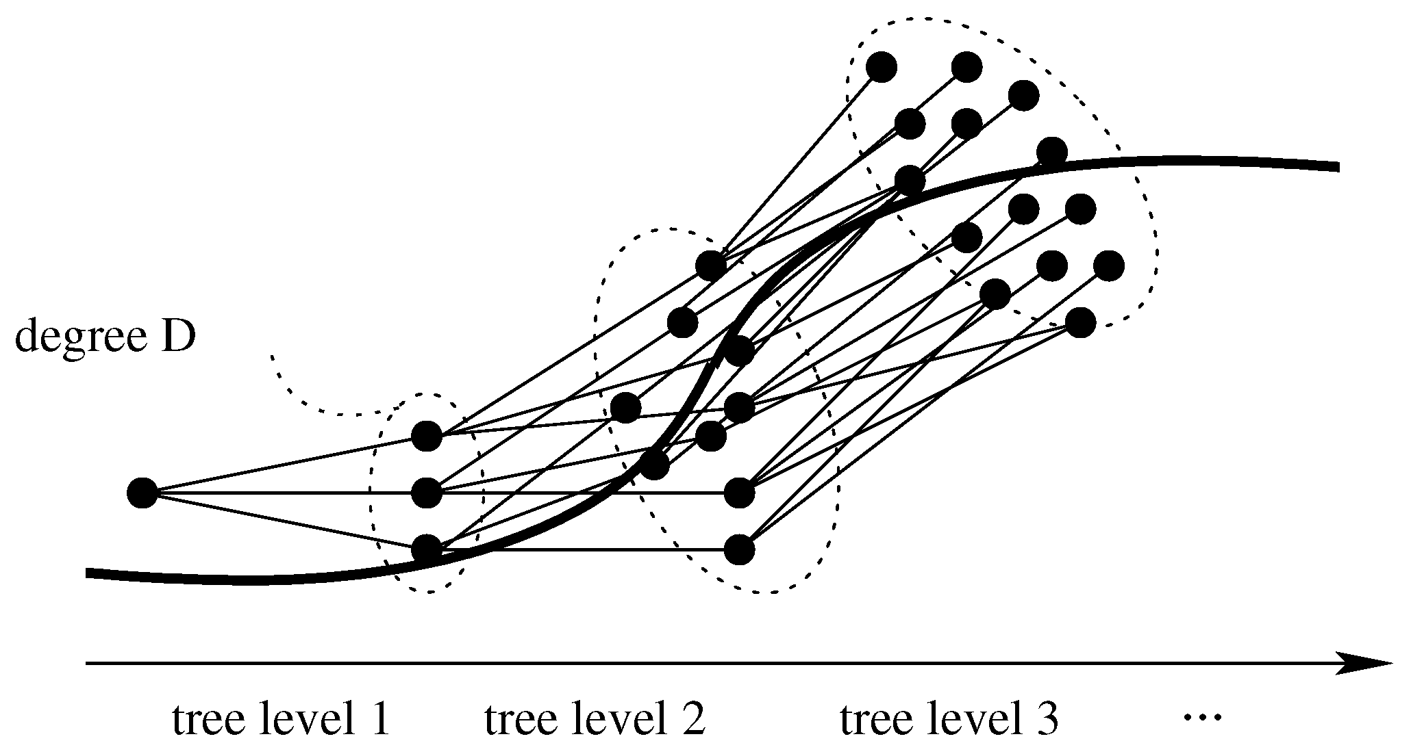
Figure 3, trajectories are organized as a tree of height
H and degree
D. This tree includes all physically feasible paths taken into consideration. Among them, the best one is finally extracted based on a specific cost function. Algorithm 1 calls functions
drawSample and
expand once for every tree edge. This meas that the algorithm performs several basic steps equal to:
formulation easily derived by using the geometric progression.
In a highly parallel environment, it is somehow immediate to organize tree construction on a level-by-level basis using one thread to generate each single parent-to-child edge (trajectory). As for each tree level
i,
calls to functions
drawSample and
expand will be made in parallel, the concurrent algorithm will be bounded by
H basic steps. Obviously, in a many-thread environment one of the main issues is how threads are synchronized and how they exchange information among them. Following this idea,
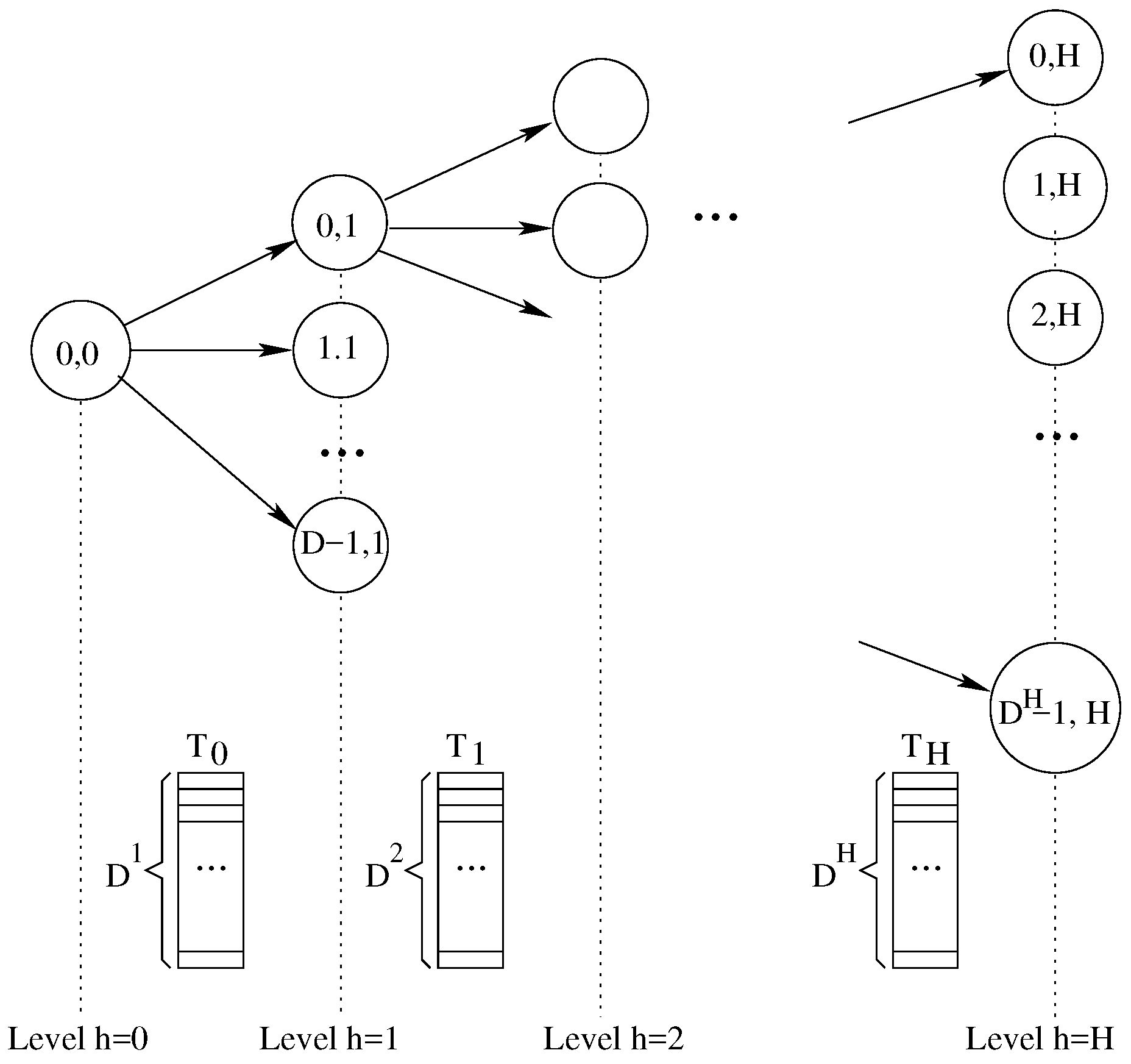
Figure 4 revisits
Figure 3 to show how the logic relationship among threads and how the overall data structure is organized.
Figure 4 shows the data array
used at each level.
From the logical point of view, each
is a texture array, containing
cells for each tree level
h. From the implementation point of view, all
textures are organized as a 2D matrix to exploit the 2D caching of the GPU. Threads refer to them using a 2D matrix index notation whereas in our logical explanation we often refer to a single index access. With this approach each tree level represents a set of parents for the next level and a set of children for the previous one. Data array at level
i is used to save the appropriate data to pass from threads at level
i to threads at level
. Each array length is equal to the number of tree nodes at that specific tree level. The array size grows exponentially, being 1,
D,
,
,
…,
. The following relations hold for parent and children indexes: a node
i at a level
j has a parent from level
and
D children at level
. The correspondence among those node indexes is the following:
Notice that this relationship is also a key aspect within the CUDA environment as each thread, given its position within the block-grid, has to save the computed data for its D children.
5.2. Data Structures and GPU Memory
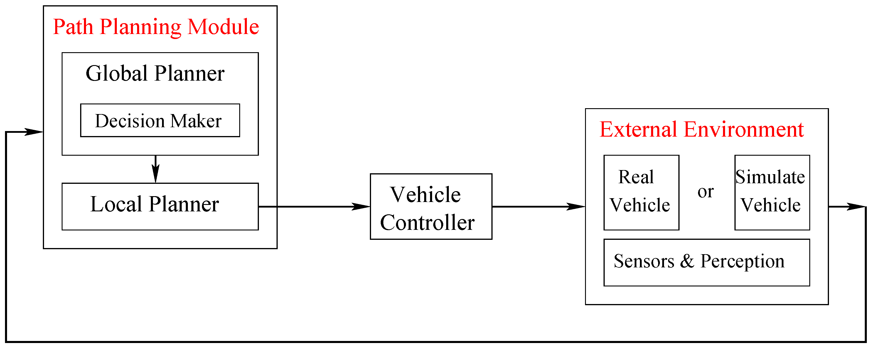
Maps are built by the data fusion module which is external to the path planner. We consider map creation, manipulation, and transfer somehow outside the scope of the present paper. Anyhow, we need to keep into account all memory and CPU costs to perform such operations to properly synchronize our threads. As the data fusion module does not share any memory with the path planner, a critical aspect of the system is how to make the path planner communicate with the outside world. If we suppose that the data fusion module organizes its data as grid maps, those maps have to be transferred within the path planner and updated frequently, as a high refresh rate guarantees a better precision and a more dynamical behavior with respect to obstacles. This in turn also means to have large memory transfer costs and high memory occupation. For the above reasons, we decide to use a surface as a Read/Write data structure exploiting caching to optimize accesses. Working on surface memories has several performance benefits compared to using global memory.
In our implementation maps are accessed to evaluate the quality of our path, i.e., the cost of each position along the path. As we must represent the environment around the car dynamically changing along time, we use a different map for each tree level expansion.
In our framework, maps are represented as an image with a resolution of
pixels. Each pixel is described by a
float value. Map resolution is
m meaning that a space of 500 m can be represented. Considering the resolution power of our sensors (see
Section 6) maps are more than sufficient to represent the neighboring area.
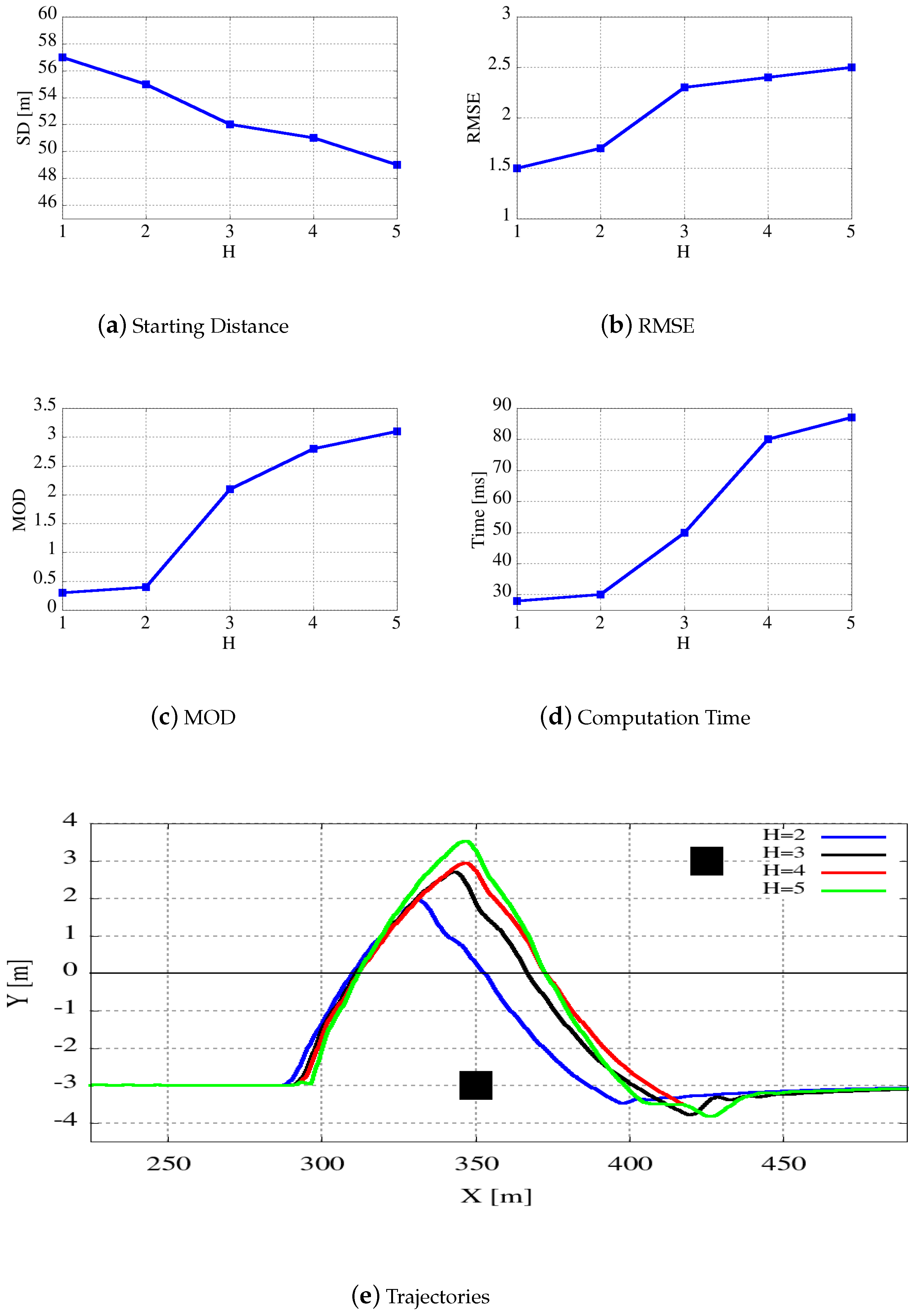
We use GPU textures to store maps efficiently. As in texture memories each pixel is represented using the 4 RGBA channels (R, G, B and A), i.e., it is represented on 4 floating point values, we simultaneously represent 4 maps on a single texture by compressing 4 pixel floating-point representations into a unique RGBA field. As a consequence, a single texture in sufficient to encode all information required by an expansion tree with height . For tree with , one possibility would be to use more than one texture to represent the required number of maps. However, we experimentally noticed that for expansion trees higher than , all estimated maps become so approximated (This approximation is due to different reasons, such as the sensor inaccuracy and the erratic behavior of many objects present in the scene, e.g., pedestrians) that they loose their meaning. For that reason, when we analyze the space for a number of tree level higher than 3, we re-use the map for for all higher levels.
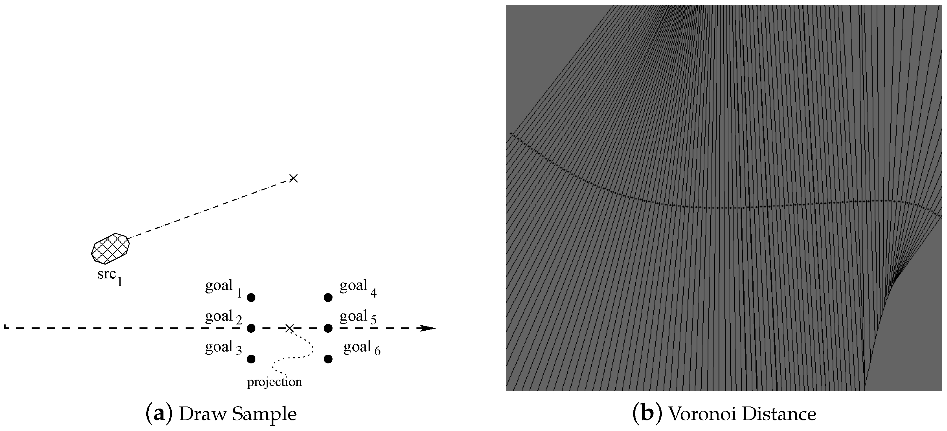
In addition to occupancy grid maps the data fusion module sends to the path planner a mathematical path description together with the associated Voronoi diagram (In mathematics, a Voronoi diagram is a partitioning of a plane into regions based on distance to points in a specific subset of the plane. That set of points (called seeds) is specified beforehand, and for each seed there is a corresponding region consisting of all points closer to that seed to any other. These regions are called Voronoi cells). The drawing sample procedure, in both CPU and GPU versions, uses the Voronoi diagram for the generation of reference points. The procedure is the following one. When the car is not on the path and it is physically impossible to select a goal on the path, the algorithm selects a feasible goal and then it approximates such a goal with the closest point on the path. Finding the closest point on the path to a given goal point (in all steps) would be really time consuming. For that reason, we use Voronoi diagrams creating “Voronoi cells” including the set of points closer to the desired “Voronoi seeds” (i.e., the given goals).
The data structure containing the Voronoi diagram is an RGBA texture of cells containing one short type. In the case of GPU implementation this diagram has to be transferred from host to a surface in the device memory. This process is expensive.
The basic data item necessary to compute a new tree edge includes the LVS and the steering angle, as well as additional information related to the current node cost. Each one of those data items requires 4 real values, i.e., 4 objects of type float4 in CUDA. In our application all kernels share a common data structure. This can be stored on the global memory but with performance penalties.
The data structure is pre-allocated and overwritten at each execution of the planning cycle, and, as introduced in
Figure 4, it can be seen as a set of layers, one for each tree level. Each layer stores all shown data, whose number depends on the current level.
5.3. High Level Algorithm
Our concurrent version of Algorithm 1 replaces the main iterations at lines 7 and 9 with concurrent thread computations. The overall work-load is then naturally partitioned in three conceptually independent tasks. Each of these tasks is implemented by a separate CUDA kernel:
The drawSampleKernel function computes reference nodes and speeds. This kernel, starting from source nodes, computes reference nodes for the second kernel and stores them in the surface memory.
The expandKernel function generates trajectories. This second kernel reads from the surface pair of source and reference nodes, and it computes the closest node according to the vehicle kinematic model. Results are made available in the surface memory for the next execution of the other two kernels. A cost is stored for each node, keeping into account the node’s parent cost.
The computeCostKernel function computes the final path. This kernel efficiently identifies the minimum cost node, and the best physically feasible path to the root.
Algorithm 2 presents our concurrent version of Algorithm 1.
Lines from 1 to 4 follow the sequential algorithm. On line 5, function mem2surf stores the required data from the CPU memory to the GPU surface memory. Within the main loop (line 6), the application runs twice groups containing D threads for a total of threads per cycle. The first set of threads runs through the drawSampleKernel function, and the second set runs through the expandKernel code. Those kernels are run in sequence, and are logically kept separated. This is because we want to keep both kernels simple enough, and to avoid branches such that the SPMD programming style is preserved.
| Algorithm 2 Highly-parallel (i.e., many-core) top-level path planner algorithm. |
Concurrent Planning cycle- 1:
, - 2:
, - 3:
=simulate (n, f, g, , ) - 4:
, - 5:
mem2surf (surf, ) - 6:
for to do - 7:
drawSampleKernel (, , ) - 8:
expandKernel (n, f, g, , , , , ) - 9:
end for - 10:
computeCostKernel () - 11:
= minimum cost node at leaves - 12:
= edge in tree level 1 leading to - 13:
return
|
Please remind that to avoid excessively long waiting times, all threads within the same kernel should execute in close time proximity with each other. Anyhow, the CUDA run-time system satisfies this constraint by assigning execution resources to all threads in a CUDA block as a unit, that is, when a thread of a block is assigned to an execution resource, all other threads in the same block are also assigned to the same resource. This ensures time proximity of all threads in a block and prevents excessive waiting time during barrier synchronization.
Moreover, to enforce regularity to all computations performed along each tree path, we avoid tree pruning even when certain edges are not useful anymore (for example, when an obstacle is too close to the computed path).
Another main issue of the algorithm is thread parallelism. For each tree layer h, with h starting from 0, we have concurrent threads. As we suppose to set , we will have threads running in parallel. As in our experiments, we used a GPU with 1664 cores, its parallel capability will saturate with . As we build the tree in a breadth-first way, this also means that we obtain the maximum parallelism in the last level whereas the parallelism is quite low during previous levels. To further increase the parallelism obtained, we have schemes in which the degree D is trimmed during the process, being larger during lower tree levels and higher for higher tree levels.
The first two kernels are executed sequentially, one after the other,
H times. Only when the tree is complete, the third kernel (see description in
Section 5.6) is launched. To efficiently run those two kernels, we organize our data structure as previously described, i.e., as a sequence of arrays containing nodes belonging to the tree and stored within surface memories. Working on surface memories has several performance benefits compared to using global memory.
Threads executed by different kernels share data and logically relate to each other using the same data structure.
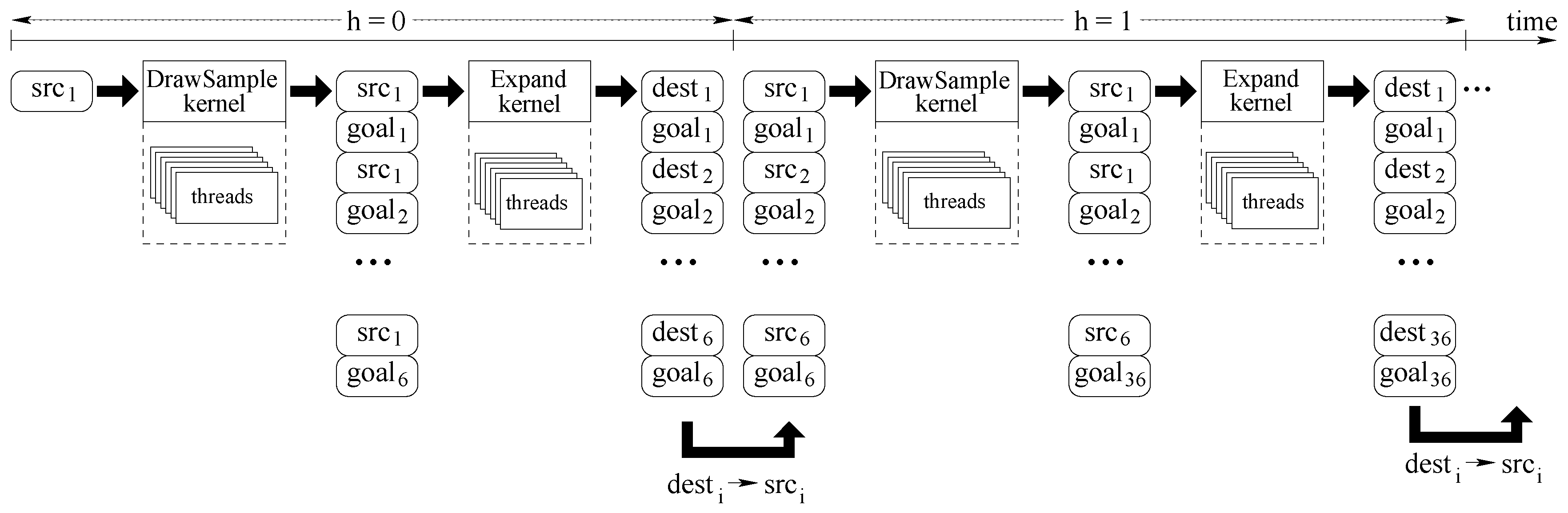
Figure 5 illustrates the communication between threads. In this picture, time flies from left to right, and we highlight how working threads at level
generate information for the working threads at level
. We suppose
.
At the very beginning, the algorithm concentrates only on the tree root representing the initial vehicle position. This position is stored in a single data record named
src. The first kernel
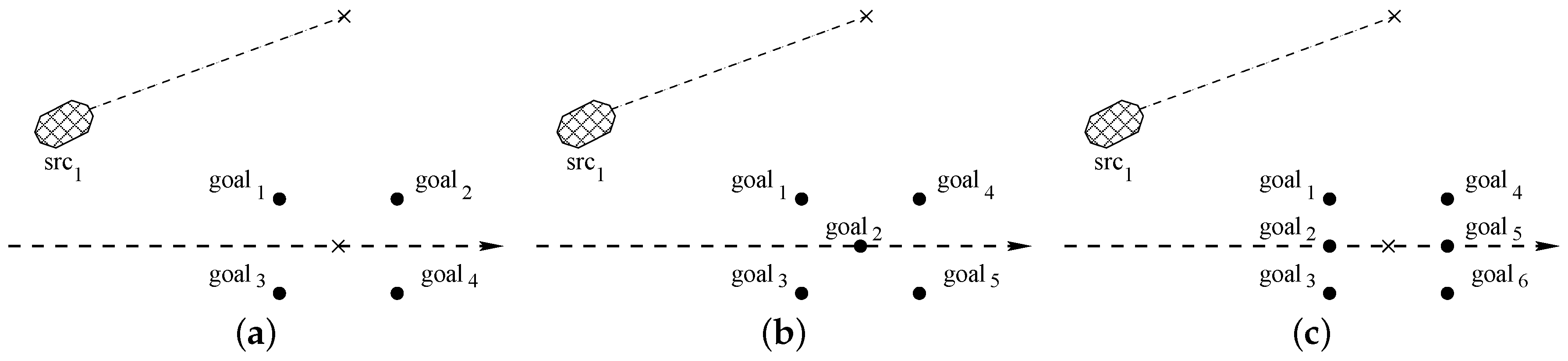
DrawSampleKernel evaluates the first set of 6 target points. To perform this step, as represented in
Figure 6a, the initial vehicle position is projected along the current path, and then orthogonal to the desired path, to find
D (6 in the picture) projected points.
Notice that as the planner is running over and over again to compute paths in close proximity of one another, orthogonal projections must be computed and recomputed for many points close to the vehicle. To avoid those re-computations and to make
DrawSampleKernel more time efficient, all orthogonal projections for dense points around the vehicle are computed during the map generation for all maps points at fixed time intervals. This is allowed by a proper use of Vonoroi maps.
Figure 6b is a logical representation of the Voronoi map, where for each point
p, the segment passing from
p and orthogonal to the path identifies the point on the path closest to
p. Each Voronoi map is stored into a texture of size equal to
pixels. Within the Voronoi map, each pixel is represented with 4 float values stored as an RGBA information. The first float indicates the index of the orthogonal projection path point stored within the texture path. All other float values store the angle of the tangent to the path and its orthogonal direction. These data are used by the kernel to compute the goals. Each map includes the GPS coordinates stored within the first top-left pixel. This pixel also specifies the pixel density within the map, i.e., the real distance between two points. This density is a function of the vehicle speed at the moment the map is generated by the global planner. Each thread reads this information and it is then able to compute the lookahead position on the map. Please note that as each map may serve several path planning cycles, it has to be large enough to include all lookahead positions computed within the next few cycles.
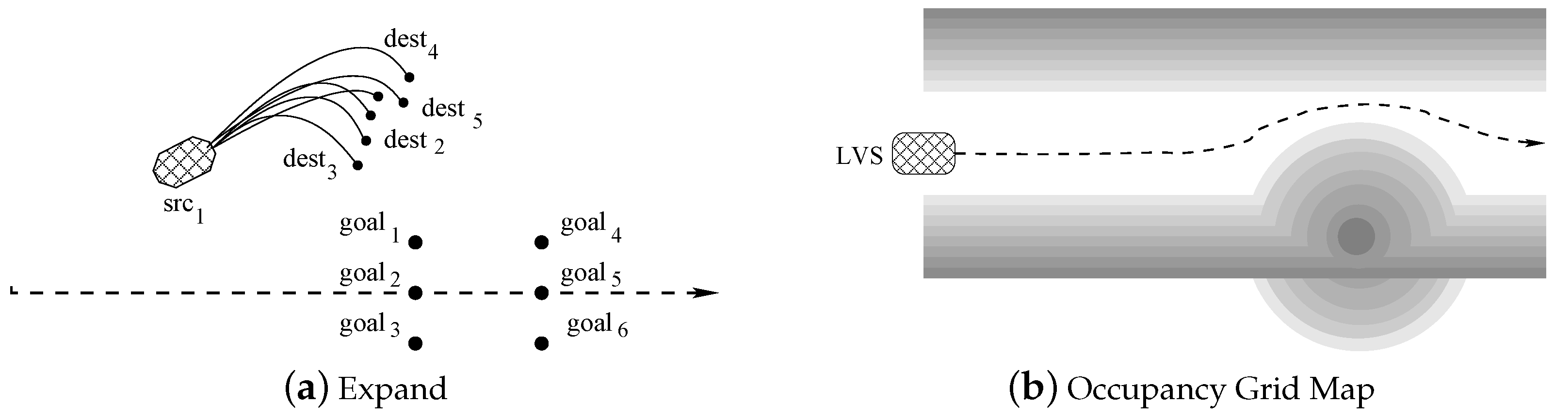
Figure 5 shows how kernel
DrawSampleKernel modifies the memory structure to set-up all required data to run kernel
Expand. Record
src is expanded into 6 record pairs
src-
goal. For each couple,
goal is the target positions (the ones represented in
Figure 6a), and
src is the same source, common to all trajectories that must be computed by kernel
ExpandKernel. When the second kernel
ExpandKernel runs, each
src record is replaced by the simulated destination position
dest. In this way, those destinations will be considered as new sources during the next algorithm iteration. This step is also represented by
Figure 7a, whereas
Figure 7b represents a mock grid map and a possible vehicle trajectory. Notice that at the end of our tree construction
dest are the final vehicle positions. Then each path from
src to a
dest implicitly includes the set of commands (generated by
ExpandKernel) that are necessary to reach a destination that, at least theoretically, should coincide with the corresponding
goal at
. Unfortunately, the algorithm just approximates desired paths. As a consequence, we store pairs
dest-
goal at the end of step
. When the second iteration of the loop at line 6 (the one with
) of
Figure 5 starts the 6 destination points
dest found during the previous iterations become source points
src. The second iteration will proceed as the previous one, but starting with
points procedure
drawSampleKernel will generate
points, and procedure
expandKernel will target them.
5.5. Function expandKernel: Computing Path to Target Nodes
Following
Section 5.1, at tree level
i a thread group of size
D is launched for each pair
. Each thread executes the kernel described in Algorithm 4. For each group the source node is read from the surface, whereas the reference node for each thread
is the one computed by the first kernel.
Function expand is the same of Algorithm 1. The output of expand is the reached point () using functions f and g and represents the source node for the following execution of Algorithm 3.
Line 3 is in charge of computing the cost of a generated node and the corresponding edge. Function
computeWeightAndCollision computes node costs. Each node has a cost that derives from its parent node cost and its position within the grid map. For this kernel, grid maps have a structure similar to the one described in
Section 5.1. Nevertheless, these grid maps have to serve function
expand for
H consecutive calls, corresponding to
H tree levels of the expansion tree. Each map has thus to foresee all object movements within
time unit. As we represent each pixel with 4 RGBA float values, we are able to represent grid maps up to 4 unit of time. If the
, the last map is reused by all kernel calls following the fourth one. Notice that this choice does not invalidate results, as in any case the last map is the one in which the trajectory is foreseen less precisely, and thus reusing it does not entail larger errors.
We use
exponential averaging to compute new costs, given higher weights to more accurate estimated positions, i.e., nodes closer to the root. For a new node at level
h the cost is computed based on the cost of all nodes along the path leading to this node from the root:
where
,
is the coefficient for the closest estimate (after
time units), and
is the farther estimate (after
time units). The destination node is marked as unfeasible when required. This essentially depends on how the grid maps are generated and on how the trajectory is placed on such a map.
Function
surfaceWriteTree writes nodes on the surface to set up all required information for the next iteration of the main cycle of
Figure 2. Each thread works on one tree layer overwriting old information (all source and goal points written by function
expand) with source and destination points.
| Algorithm 4 Kernel2: expand |
expandKernel- 1:
= surfRead () - 2:
(, ) = expand (, f, g, , ) - 3:
computeWeightAndCollision (, ) - 4:
surfaceWriteTree (, , , )
|
5.6. Function computeCostKernel: Selecting the Best Path
Once all trajectories have been computed and their costs evaluated, tree leaves contain the cumulative cost of the entire path leading to them. The next step is to select the most promising trajectory, i.e., the one with the smallest cost. Finding a minimum entails a linear visit, but implementing a linear visit on a multi-core architecture can lead to several inefficiencies. As suggested by many other authors (see for examples Chen at al. [
14] for considerations on many-thread sorting) we trade-off time-efficiency and accuracy.
Figure 5 describes our bucket sort-inspired algorithm. It works as follows.
The cost function computes real cost values for each leaf. Let us suppose those values are included in a specific interval . First of all, we divide this interval into N classes. In this way, each class has a width equal to . Then, we build a pseudo-histogram by inserting in each class all leaves with a costs belonging to the class interval. To populate the histogram, i.e., to insert each leaf in the proper class, function computeCostKernel runs one thread for each tree leaf.
Each thread behaves like function populateHistogram in Algorithm 5. Each thread is in charge of placing the leaf identifier into the corresponding histogram class. To do that, it gets the leaf identifier and the leaf cost from its leaf (lines 1 and 2). Given the leaf cost , line 3 computes the index of the bucket () the leaf belong to. As all threads work in parallel, we must guarantee a proper synchronization among them, such that only thread can modify a class at any given time. To do that, we use the atomic CUDA function atomic_add (see line 4) to add the node identifier to the proper class bucket (properly initialized to zero). As the CUDA atomic_add returns the original value for each addition, we always know whether the added value is the first one or not (line 5). In the first case, the thread leaves the bucket equal to the leaf identifier and then it terminates. Otherwise, it subtracts the same leaf identifier from the bucket (line 6) such that when all threads have terminated each class bucket stores only one identifier value, corresponding to the node placed in the bucket first.
Once all threads running function populateHistogram have terminated, function computeCostKernel runs one more kernel with a single thread. This thread performs a linear search in all buckets of the histogram looking for the leaf with the smallest cost, i.e., the one stored in the leftmost bucket.
Notice that in this case linear search is performed only on those classes that have no representative, as the algorithm stops on the first non-empty class. This makes our algorithm much faster than a standard linear search. Moreover, we select the number of classes N as a function of maximum available number of threads available and the desired approximation. For example, if our costs belong to the interval , and we select , we generate a histogram with 1000 classes, and we obtain a class width and an accuracy equal to .
As a last step, function computeCostKernel returns the selected node plus the the entire path leading to it from the tree root.
| Algorithm 5 Histogram Computation. |
populateHistogram- 1:
= retrieveNodeIndex() - 2:
= retrieveNodeCost() - 3:
= - 4:
= atomicAdd(bucket[], ) - 5:
ifthen - 6:
atomicAdd(bucket[], ) - 7:
end if
|

 ,
, 


