The Improved Division-Less MT-Type Velocity Estimation Algorithm for Low-Cost FPGAs

Abstract

Advanced motion control applications require smooth and highly accurate high-bandwidth velocity feedback, which is usually provided by an incremental encoder. Furthermore, high sampling rates are also demanded in order to achieve cutting-edge system performance. Such control system performance with high accuracy can be achieved easily by FPGA-based controllers. On the other hand, the well-known MT method for velocity estimation has been well proven in practice. However, its complexity, which is related to the inherent arithmetic division involved in the calculus part of the method, prevents its holistic implementation as a single-chip solution on small-size low-cost FPGAs that are suitable for practical optimized control systems. In order to overcome this obstacle, we proposed a division-less MT-type algorithm that consumes only minimal FPGA resources, which makes it proper for modern cost-optimized FPGAs. In this paper, we present new results. The recursive discrete algorithm has been further optimized, in order to improve the accuracy of the velocity estimation. The novel algorithm has also been implemented on the experimental FPGA board, and validated by practical experiments. The enhanced algorithm design resulted in improved practical performance.

1. Introduction

Nowadays, digital programmable circuits such as FPGAs are used widely for many industrial applications [1]. They offer possibilities for integrating complex hardware systems and their interfaces into a single FPGA chip. FPGA devices have reached a high maturity level in terms of performance, power consumption, and cost, which makes them suitable for different application fields [2] that involve sensor systems [3,4], control systems [5,6], haptic interfaces [7,8], robotics [9,10,11], and other advanced electronic devices for signal processing and communications, e.g., [12,13,14,15]. They can also be useful for advanced velocity estimation methods, since they can easily be designed for custom signal conditioning and provide fast dedicated digital logic [16]. FPGAs can also ensure highly accurate and short sampling periods, which are required for advanced motion control applications. A short processing time of control algorithms is also possible; however, the feature-rich FPGAs have overwhelming resources that are required for performing complex computation algorithms [17,18] yet are still expensive, which may prevent their further use in low-cost applications. One of the challenges in the electronics industry nowadays concerns fitting complex circuitry into small spaces. Thus, the current FPGA development is also directed to smaller design solutions, with low-power consumption in a low-occupied space at low cost, while maintaining a solid performance level [19]. Such low-power, small-size, and cost-optimized FPGAs introduce the possibility of developing new cutting-edge solutions, e.g., in the area of smart sensors and other smart devices [20].

The importance of velocity feedback for the closed-loop control of mechatronic systems has been well-known for many decades. Typical feedback devices in the control systems for servo drives in automation are incremental encoders [21]. These control loops must allow smooth motion in a wide range from high speed to low speed. Incremental encoders, which are typically mounted on a motor shaft, can provide high resolution and high accuracy in position measurement, which makes them an optimal option for such a purpose [22]. On the other hand, the maturity level of digital electronics technology has enabled their use not only for position feedback, but also for velocity feedback [23]. They generate digital pulse train signals while their shaft rotates, which is coupled with a motor shaft. However, precise feedback information is essential for motor control, e.g., in machine tools, robotics, autonomous systems, and medical mechatronics. Regardless of the motor control methods, the accuracy of feedback information has a major influence on the control performance. Furthermore, advanced motion control applications require highly accurate wide-range velocity information with high bandwidth [24,25]. Thus, since incremental encoders can only generate a pulse train with its frequency related to the shaft velocity, a suitable estimation algorithm should be applied in order to obtain smooth velocity information. Although there has been extensive past research related to this issue over the past few decades [26,27], new emerging applications in robotics and other areas with cutting-edge requirements foster further intensive research in this field, e.g., the motion control of hydraulic actuators [28], pneumatic actuators [29], haptic interfaces [30], mobile robots [31], robot manipulators [32], humanoid robots [33], and collaborative robots for safe physical human–robot interaction [34], automotive applications [35], etc. Since the performance of a velocity control loop is related strongly to the quality of the velocity feedback information, achieving a smooth, high-bandwidth velocity estimate, which is required for oscillation-free high-bandwidth control loops, still presents quite a challenge.

The motor velocity is conventionally obtained by counting encoder pulses in a fixed sampling period. However, despite its simple implementation, it cannot provide precise velocity information in the case of a low-resolution encoder or short sampling periods. Furthermore, in these cases, it produces large quantization errors due to the spatial position quantization that is inherent in incremental encoders. Therefore, more advanced estimation methods should be applied in order to obtain smooth velocity information. They can be classified as model-based or non model-based methods [36]. Model-based methods use models of the dynamic systems for which the velocities are to be estimated. In general, these methods rely on a mechanical system model, which must be accurately available. This is often a significant obstacle in practice, since it may be difficult to obtain, or it is time varying, or it may be unknown or uncertain. In these cases, non model-based methods can be adopted. These methods are based on data processing techniques that use only measured data without any of the information of the motion system. The aforementioned simplest conventional method is usually referred to as the M method. Due to its problems at low speed, filtering of the data may be applied, although it introduces phase lag, which is undesired in advanced motion control applications. The alternative T method can be utilized instead, in which the time interval between two adjacent encoder pulses should be measured by counting high-frequency clock pulses. Then, the velocity information is obtained by the reciprocal of the measured time interval, i.e., by arithmetic division. Although the method can provide fine velocity estimation at low speed, it is prone to errors at high speed. Thus, the main stream of the velocity measurement methods combines the M method and the T method. Since the pioneering work of Ohmae [37], the MT method has been applied widely, because it works well within wide speed ranges. The method counts the number of encoder pulses in a sampling period and measures the time interval between the boundary encoder pulses by counting the high-frequency clock pulses. Then, the velocity information is computed by arithmetical division of the number of encoder pulses over the time interval. Some variations of the MT method appeared in [38,39,40]. Further research deals with performance improvement of the MT method and its enhanced robustness to the encoder imperfections and hardware inaccuracies [16,25,41,42]. The time stamping of encoder pulses presents a generalization of the MT method [43,44]. Here, the velocity is estimated by a polynomial fitting through a number of time-stamped encoder counts, which significantly increases the computation complexity.

The MT method consists of signal reading and data processing. Common implementations may conveniently combine an FPGA for the hardware part of the method, which involves signal acquisition, counting encoder pulses, and counting clock pulses, and a computation engine such as a DSP processor for processing the software algorithm of the method in real time [16,26,45,46]. Such a heterogeneous system structure significantly increases the system complexity. Thus, it may be convenient to implement the velocity estimation method on an FPGA as a whole. However, one should note that the algorithm of the MT method involves arithmetic division. Although it is easy to perform the division operation by the DSP, on the other hand, it is particularly difficult for FPGA-based embedded electronics, i.e., its implementation is characterized with high computation latency and a high consumption of FPGA resources [47,48,49]. Although modern advanced and feature-rich FPGAs with overwhelming resources are capable of performing such tasks, this solution raises the cost drastically, which may be unacceptable in many cases. Therefore, for the efficient implementation of the MT method on an FPGA, it is necessary to eliminate the division operation that is inherent in the conventional algorithm. Then, its implementation will be possible on cost-optimized FPGAs as well. Such FPGAs, on the other hand, can embed digital multipliers, or so-called DSP blocks, that perform arithmetic multiplication and addition efficiently [50]. Therefore, division-less algorithms can be implemented easily in an efficient way with high-speed processing. Zhu [51] proposed a simple solution that seamlessly combines the M method and the T method. It applies a sophisticated mechanism with two counters and an accumulator; however, it requires the execution of the algorithm continuously in every clock cycle, which increases the resources and power consumption, and thus is undesired [49].

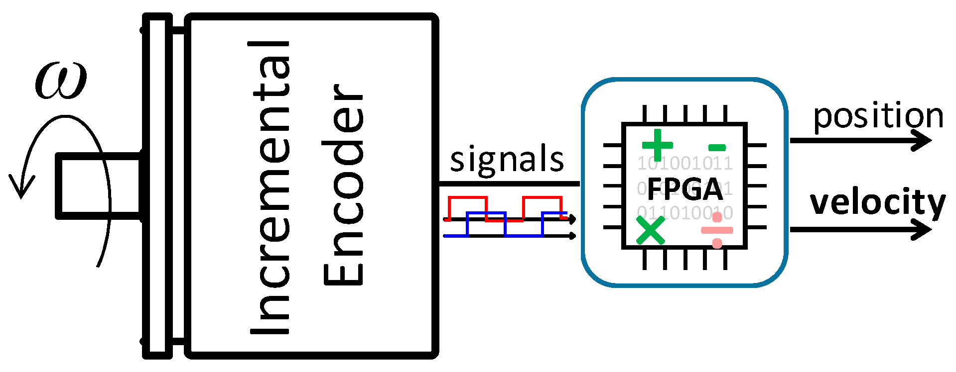
In our research, we are concerned with the efficient implementation of the MT method for smooth velocity estimation on a low-cost FPGA, as illustrated by Figure 1. We introduced a novel MT-type method in [52] that eliminates the arithmetic division from the algorithm, while preserving the utmost accuracy of the conventional MT method. Thus, it is convenient for implementation on small-sized cost-optimized FPGAs. The method is abbreviated as a DLMT (division-less MT). It involves multiplication and addition, which are the only required arithmetic operations in the real-time calculation. However, the method is recursive; thus, stability and convergence should be considered strictly in the design phase. It has been found out that the basic method algorithm can suffer from instability at low speed in the case of blank sampling intervals when encoder pulses are widespread. Therefore, it has been adapted properly to guarantee asymptotically stable performance at all speed ranges [53]. Such a generalized DLMT method has been abbreviated as the GDLMT method. The method was implemented on the FPGA and verified experimentally. Although the method performed well in practical experiments, it is represented as a time-varying discrete system of the second order that may generate a weakly damped fluctuated response. Thus, in this paper, we revise the algorithm to reduce the system order, and propose the division-less algorithm with the simplified dynamics of the first order. We show that, inherently, it significantly reduces undesired fluctuations during the transient phase. The stability and convergence is also discussed theoretically and proven formally. Furthermore, the estimation error is reduced as well, which is confirmed by experimental results.

2. Materials and Methods

2.1. The Principle of the MT Method

The MT method for velocity measurement can be described by the following formula [26]:

$${\widehat{v}}_k^{MT}=\frac{x_k-x_{k-1}}{T_s+\delta t_{k-1}-\delta t_k}$$

(1)

where ${\widehat{v}}_k^{MT}={\widehat{v}}_{}^{MT}(t=t_k)$ and $x_k$ are the estimated velocity in the k-th sampling interval and the encoder position sampled in the k-th sampling instant, respectively. $T_s$ is the sampling period, and $\delta t_k$ is the time elapsed between the time instant of the most recent encoder pulse in the current sampling interval ($t_k^p$) and the current sampling instant ($t_k$), such that it can be calculated as (for details, see Figure 2):

$$\delta t_k=t_k-t_k^p$$

(2)

where $t_k=k{T}_s$, and $x_k=x(t=t_k^p)$ is the encoder position reading. However, it is not available for processing before the current sampling instant ($t_k>t_k^p$). Note that ${\widehat{v}}_k^{MT}$ equals the average velocity ${\overline{v}}_k^p$ on the time interval $t_{k-1}^p\le t\le t_k^p$, such that ${\widehat{v}}_{}^{MT}(t=t_k)={\overline{v}}_k^p$. Thus, the measurement interval matches the interpulse interval $T_k^p$ and can be calculated as:

$$T_k^p=t_k^p-t_{k-1}^p=T_s+\delta t_{k-1}-\delta t_k$$

(3)

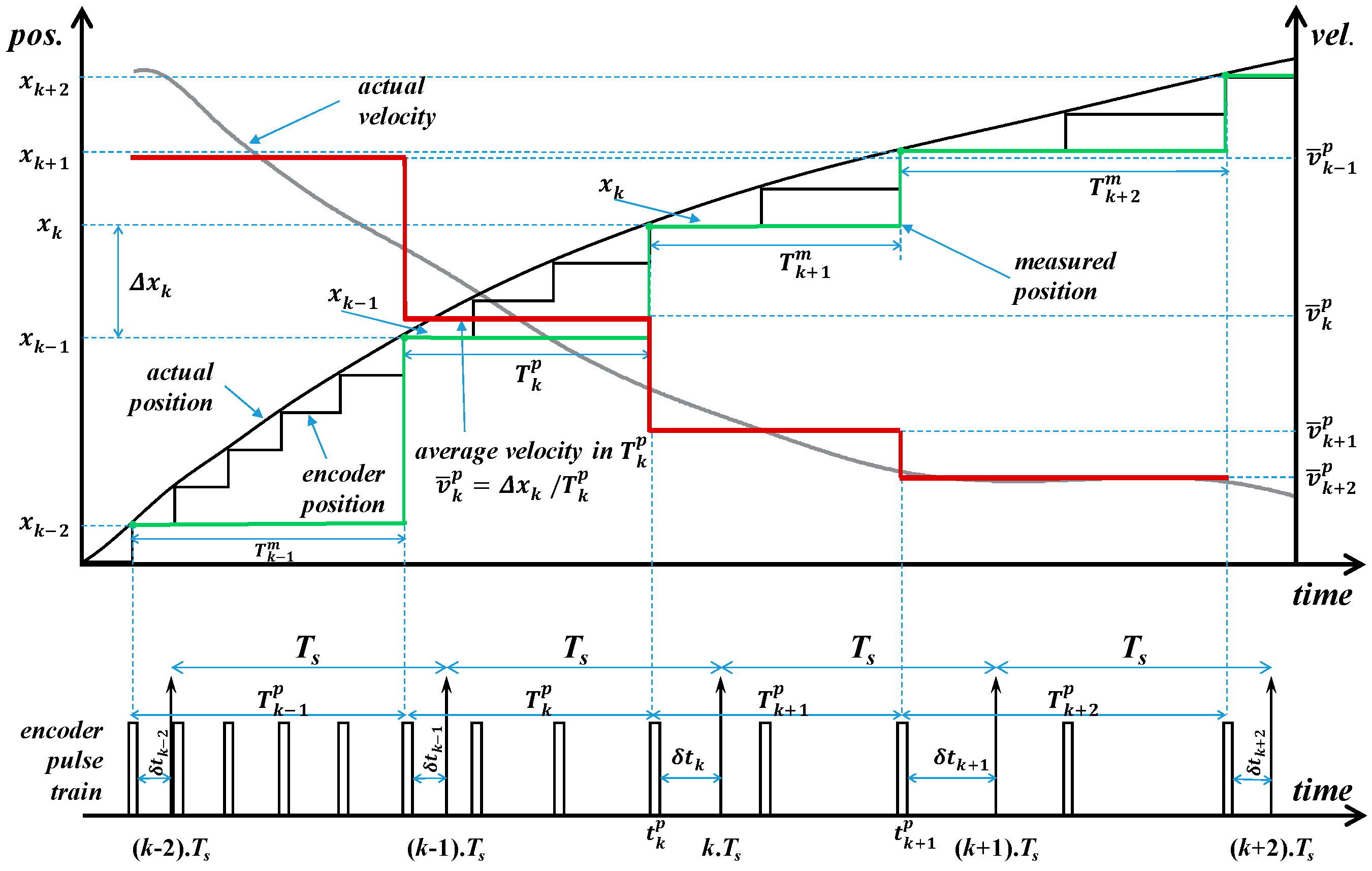
In order to implement the MT velocity measurement method in practice, it is required to measure the position pulse train from the incremental encoder, and clock pulses that enable the determination of the time interval measurement between the most recent (boundary) encoder pulses in two consecutive sampling periods. Figure 2 shows the timing diagram of the conventional MT method with the actual position trajectory, encoder position, encoder pulse train, sampling intervals with the constant period T_s, and variable measurement intervals $T_k^p$. It is easy to figure out that the update of the velocity ${\widehat{v}}_k^{MT}$ is delayed with reference to the average velocity ${\overline{v}}_k^p$. Moreover, the average velocity within the most recent sampling period may differ from the latter value.

In the following, we derive the estimation error, which is produced by the MT method. If we define the average velocity ${\overline{v}}_k^a$ on a sampling interval such that:

$${\overline{v}}_k^a=\frac{x_k^a-x_{k-1}^a}{T_s}$$

(4)

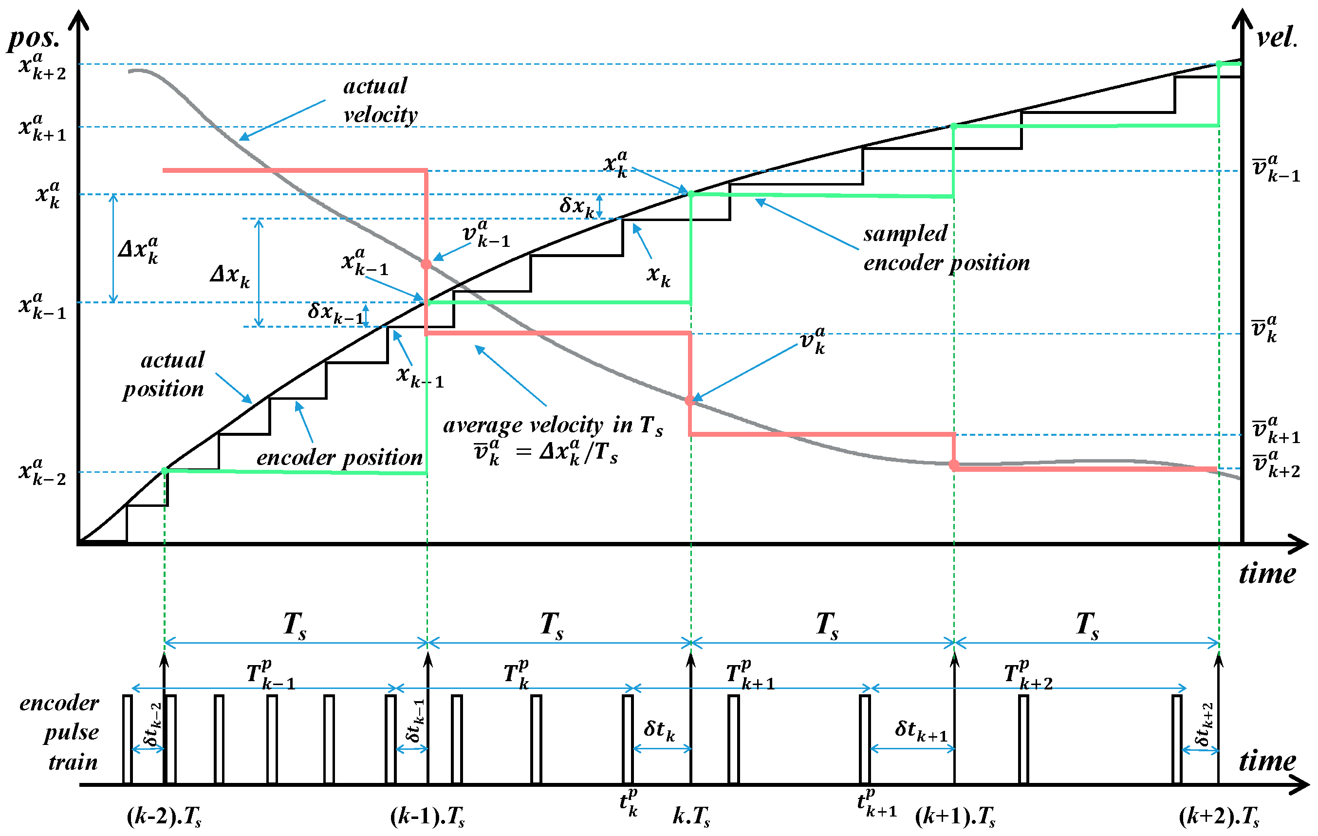
Then, we can assume that the average velocity ${\overline{v}}_k^a$ could be the best possible velocity estimation in the case of accurate position reading at the sampling instants. If we further consider $x_k=x_{k-1}^a+(T_s-\delta t_k){\overline{v}}_k^a$ and $x_{k-1}=x_{k-1}^a-\delta t_{k-1}{\overline{v}}_{k-1}^a$ (see Figure 3), then, after short manipulation, we obtain:

$$T_s{\overline{v}}_k^a-\delta t_k{\overline{v}}_k^a+\delta t_{k-1}{\overline{v}}_{k-1}^a=\mathsf{\Delta }{x}_k^{}$$

(5)

Equation (1) can be rewritten as:

$$T_s{\widehat{v}}_k^{MT}-\delta t_k{\widehat{v}}_k^{MT}+\delta t_{k-1}{\widehat{v}}_k^{MT}=\mathsf{\Delta }{x}_k$$

(6)

Now, we rearrange the previously derived Equation (5), such that it yields:

$$T_s{\overline{v}}_k^a-\delta t_k{\overline{v}}_k^a+\delta t_{k-1}{\overline{v}}_k^a=\mathsf{\Delta }{x}_k^{}+\delta t_{k-1}\mathsf{\Delta }{\overline{v}}_k^a$$

(7)

If we define:

$$e_k^{MT}={\overline{v}}_k^a-{\widehat{v}}_k^{MT}$$

(8)

then, by subtraction of Equation (6) from Equation (7), which results in:

$$T_s{e}_k^{MT}-\delta t_k{e}_k^{MT}+\delta t_{k-1}{e}_k^{MT}=\delta t_{k-1}\mathsf{\Delta }{\overline{v}}_k^a$$

(9)

we get the estimation error of the MT method:

$$e_k^{MT}=\frac{\delta t_{k-1}}{T_s-\delta t_k+\delta t_{k-1}}\mathsf{\Delta }{\overline{v}}_k^a$$

(10)

If we define acceleration $a_k=\mathsf{\Delta }{\overline{v}}_k^a/T_s$ that is always bounded in practice such that $\left|a_k\right|\le a_{\max }$, then the r.h.s. (right-hand side) expression of Equation (10) is evaluated as:

$$e_k^{MT}=\frac{\delta t_{k-1}}{T_s-\delta t_k+\delta t_{k-1}}{T}_s{a}_k$$

(11)

We can evaluate its maximum absolute value considering the bounded interval $0\le \delta t_k<T_s$ as:

$$\le \frac{\delta t_{k-1}}{T_s-\delta t_k+\delta t_{k-1}}\left|T_s{a}_k\right|\le \frac{T_s}{2T_s-\delta t_k}{T}_s{a}_{\max }\le \frac{T_s}{2T_s-T_s}{T}_s{a}_{\max }=T_s{a}_{\max }$$

(12)

The estimation error of the MT method is bounded by $T_s{a}_{\max }$. The error is due to the averaging of the velocity in the most recent interpulse interval, and is caused by accelerated motion. However, it can be reduced arbitrarily by the sampling period $T_s$_, thus achieving the desired accuracy.

It is well-known that the MT method features accurate velocity measurement in a wide speed range. However, in order to obtain the velocity information, it is necessary to perform an arithmetic division in the processing hardware, since the denominator in Equation (1) is a variable time interval that must be obtained by a dedicated hardware.

2.2. The MT-Type Division-Less Algorithm of the Second Order

The simplest method for velocity measurement only counts encoder position pulses in a fixed sampling interval, and the velocity is then estimated, dividing the corresponding position increment $\mathsf{\Delta }{x}_k=x_k-x_{k-1}$ by the sampling period, i.e., ${\widehat{v}}_k^{}=\mathsf{\Delta }{x}_k/T_s$. It is called the M method.

Although the M method produces significant noise and low accuracy in the case of low velocity, it is simple, not only in terms of its hardware implementation, but also in calculus, since the division with the constant sampling period T_s can be replaced by multiplication with the constant sampling frequency $F_s=1/T_s$, which is performed easily by the processing electronics. Therefore, in order to combine the low noise and high accuracy of the MT method and low computation complexity of the M method, the authors in [52] proposed the so-called DLMT method (division-less MT method). The concept of the algorithm, which simplifies the computation complexity in comparison with the conventional MT method approach and maintains its most salient good features simultaneously, is shown in Figure 3. The main assumption is that the actual position information is available at the sampling instants $x_k^a=x_{}^a(t=t_k^{})$. However, because the encoder pulses are asynchronous with the sampling instants, this assumption cannot be realized solely by the measurement principle. Thus, the actual position at the sampling instants is estimated by the extrapolation of the encoder position as:

$${\widehat{x}}_k^a=x_k+\delta {\widehat{x}}_k$$

(13)

where ${\widehat{x}}_k^a={\widehat{x}}_{}^a(t=t_k^{})$, $x_k=x^{}(t_k-\delta t_k)$, and $\delta {\widehat{x}}_k$ are the estimated actual position at the k-th sampling instant, the recent encoder position read during the k-th sampling period, and the estimated position correction in the k-th sampling period, respectively. $\delta t_k$ is the elapsed time interval at the k-th sampling instant, since the recent encoder pulse in the k-th sampling period. The position correction could be calculated simply as $\delta {\widehat{x}}_k={\overline{v}}_k^a\delta t_k$, where ${\overline{v}}_k^a$ stands for the average velocity within the k-th sampling period, i.e., ${\overline{v}}_k^a=(v_k^a+v_{k-1}^a)/2$, where $v_k^a=v^a(t=t_k)$. Unfortunately, this value is not available in practice, and thus it should be estimated somehow. If we assume short sampling periods, then the division-free velocity estimation algorithm can be read as [52]:

$${\widehat{x}}_k^a=x_k+{\widehat{v}}_{k-1}\delta t_k$$

(14)

$${\widehat{v}}_k=\mathsf{\Delta }{\widehat{x}}_k^a/T_s$$

(15)

where $\mathsf{\Delta }{\widehat{x}}_k^a={\widehat{x}}_k^a-{\widehat{x}}_{k-1}^a$, and ${\widehat{v}}_k$ is the value of estimated average velocity in the k-th sampling period.

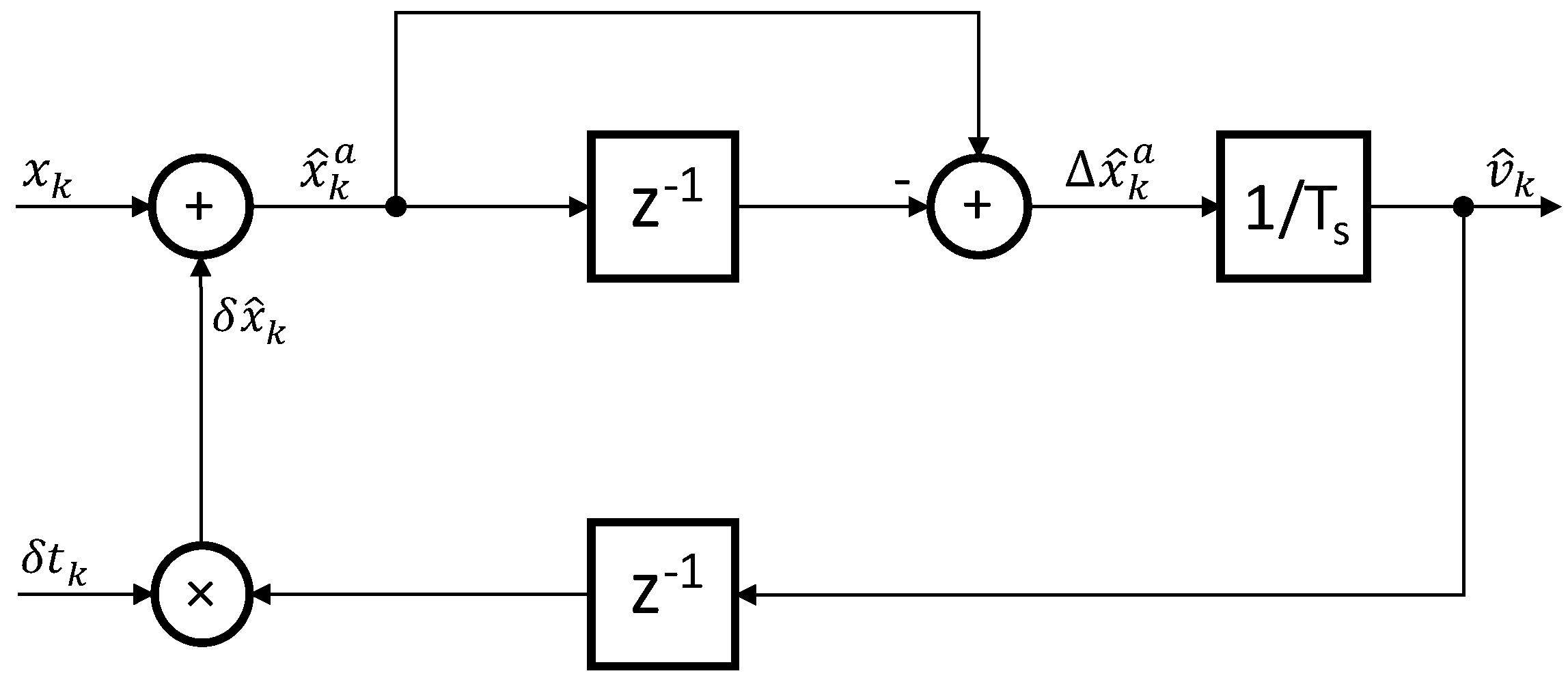
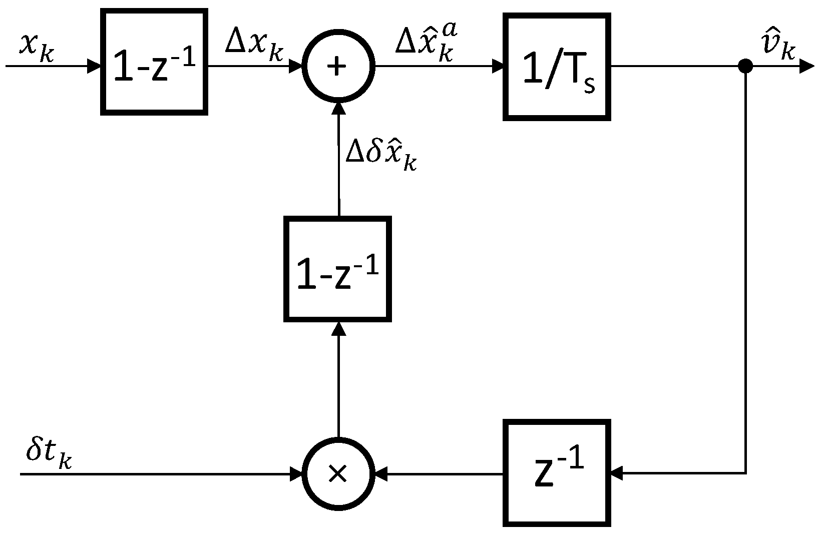
The MT-type division-less algorithm, as shown in Equations (14) and (15), can be described graphically by the block scheme in Figure 4. Obviously, the inputs in the algorithm are the sampled encoder position $x_k$- and the elapsed time intervalsince the recent encoder pulse, i.e., $\delta t_k$, whereas the main output of the algorithm is the estimated velocity ${\widehat{v}}_k$. Besides that, it can also provide the position output, which approximates the actual position at the current sampling instant, i.e., ${\widehat{x}}_k^a={\widehat{x}}_{}^a(t=t_k)\approx x_{}^a(t=t_k)$. However, one can note that the algorithm is recursive. If we can guarantee that the position estimation ${\widehat{x}}_k^a$ in Equation (14) will match the actual position $x_k^a$ closely, then the velocity estimation ${\widehat{v}}_k$ in Equation (15) will match the actual average velocity in the sampling period ${\overline{v}}_k^a$ closely. Nevertheless, the algorithm’s stability and convergence is therefore an open issue in general, and must be verified. For details, please see [52].

Further analysis focuses on the algorithm dynamics’ behavior. The input–output dynamics can be derived as [52]:

$${\widehat{v}}_k-\frac{\delta t_k}{T_s}{\widehat{v}}_{k-1}+\frac{\delta t_{k-1}}{T_s}{\widehat{v}}_{k-2}=\frac{\mathsf{\Delta }{x}_k^{}}{T_s}$$

(16)

One can note that the right-hand side expression equals the simplest M method for the velocity estimation (the position change occurred in the sampling time interval Δx_k divided by the sampling period $T_s$). Therefore, the proposed method can be understood as filtering the M method. However, the coefficients on the left-hand side of the expression are time-variant, since their values depend on the time instants of the encoder position pulses’ occurrence. Thus, the DLMT algorithm yields a linear time-variant discrete filter, which is of the second order; therefore, in this paper, the algorithm is abbreviated as DLMT2 (division-less MT-type algorithm of the second order). The DLMT2 filter in Equation (16) can be illustrated by the block scheme depicted by Figure 5.

It is easy to derive the dynamic equilibrium, which can be written as [52]:

$${\widehat{v}}_k^{eq}=\frac{x_k^{}-x_{k-1}^{}}{T_s+\delta t_{k-1}-\delta t_k}$$

(17)

One can note that the equilibrium equals the output of the algebraic MT method (1). Furthermore, the convergence dynamics can be derived as [52]:

$${\epsilon }_k^{}-\frac{\delta t_k}{T_s}{\epsilon }_{k-1}^{}+\frac{\delta t_{k-1}}{T_s}{\epsilon }_{k-2}^{}=\frac{\mathsf{\Delta }\delta t_k}{T_s}\mathsf{\Delta }{\widehat{v}}_k^{eq}-\frac{\delta t_{k-1}}{T_s}\mathsf{\Delta }{\widehat{v}}_{k-1}^{eq}$$

(18)

where $\mathsf{\Delta }\delta t_k=\delta t_k-\delta t_{k-1}$, $\mathsf{\Delta }{\widehat{v}}_k^{eq}={\widehat{v}}_k^{eq}-{\widehat{v}}_{k-1}^{eq}$ and ${\epsilon }_k$ is the convergence error:

$${\epsilon }_k={\widehat{v}}_k^{eq}-{\widehat{v}}_k^{}$$

(19)

In the following, we show the estimation error dynamics. We define the velocity estimation error:

$$e_k^{}={\overline{v}}_k-{\widehat{v}}_k^{}.$$

(20)

If we rearrange Equation (5) into:

$${\overline{v}}_k-\frac{\delta t_k}{T_s}{\overline{v}}_{k-1}+\frac{\delta t_{k-1}}{T_s}{\overline{v}}_{k-2}=\frac{\mathsf{\Delta }{x}_k^{}}{T_s}+\frac{\delta t_k}{T_s}\mathsf{\Delta }{\overline{v}}_k-\frac{\delta t_{k-1}}{T_s}\mathsf{\Delta }{\overline{v}}_{k-1}$$

(21)

then we derive the estimation error dynamics by subtraction of Equation (16) from Equation (21). It yields:

$$e_k^{}-\frac{\delta t_k}{T_s}{e}_{k-1}^{}+\frac{\delta t_{k-1}}{T_s}{e}_{k-2}^{}=\frac{\delta t_k}{T_s}\mathsf{\Delta }{\overline{v}}_k-\frac{\delta t_{k-1}}{T_s}\mathsf{\Delta }{\overline{v}}_{k-1}$$

(22)

It is obvious that the error dynamics in Equations (18) and (22) are driven by acceleration, which is manifested by velocity change. If we define acceleration $a_k=\mathsf{\Delta }{\overline{v}}_k^a/T_s$ that is always bounded in practice such that $\left|a_k\right|\le a_{\max }$, then by considering $0\le \delta t_k<T_s$, we can evaluate the r.h.s. of Equation (22):

$$\left|\delta t_k{a}_k-\delta t_{k-1}{a}_{k-1}\right|\le \left|\delta t_k{a}_k\right|+\left|\delta t_{k-1}{a}_{k-1}\right|\le T_s\left|a_k\right|+T_s\left|a_{k-1}\right|\le 2T_s{a}_{\max }$$

(23)

The latter result is very conservative; the value that is more realistic is $T_s{a}_{\max }$. However, the response of the second order filter in Equation (23) may result in overshoot; therefore, the aforementioned value cannot be considered strictly as a maximum value of the error. Nevertheless, if we assume relatively fast sampling intervals, then the velocity change in a single sampling interval can be considered negligible, and the equation’s right-hand side can be zeroed in practical advanced motion control applications. However, the stability of the system should be investigated. The stability issue of the DLMT2 algorithm has been discussed thoroughly in [52].

2.3. The MT-Type Division-Less Algorithm of the First Order

2.3.1. The Main Idea

The velocity estimation algorithm in Equations (14) and (15) can be developed further. Its accuracy is based on the accuracy of the position estimation accuracy of ${\widehat{x}}_k^a$. In order to estimate its value, the algorithm applies the best velocity value that is only available at the time of the calculation, i.e., the estimated average velocity from the previous sampling period ${\widehat{v}}_{k-1}$. However, when the calculation of the algorithm in a single sampling period is completed, then the estimation of the average velocity in the current sampling period becomes available. Thus, the estimation of the position can be improved by the estimated average velocity in the current sampling period ${\widehat{v}}_k$. Therefore, the estimation algorithm can be rewritten as:

$${\widehat{x}}_{k|k-1}^a=x_k+{\widehat{v}}_{k-1}\delta t_k$$

(24)

$${\widehat{v}}_k=({\widehat{x}}_{k|k-1}^a-{\widehat{x}}_{k-1|k-1}^a)/T_s$$

(25)

$${\widehat{x}}_{k|k}^a={\widehat{x}}_{k|k-1}^a+\mathsf{\Delta }{\widehat{v}}_k\delta t_k$$

(26)

where $\mathsf{\Delta }{\widehat{v}}_k={\widehat{v}}_k-{\widehat{v}}_{k-1}$. One can note that the improved position estimation equals:

$${\widehat{x}}_{k|k}^a=x_k^{}+{\widehat{v}}_k\delta t_k$$

(27)

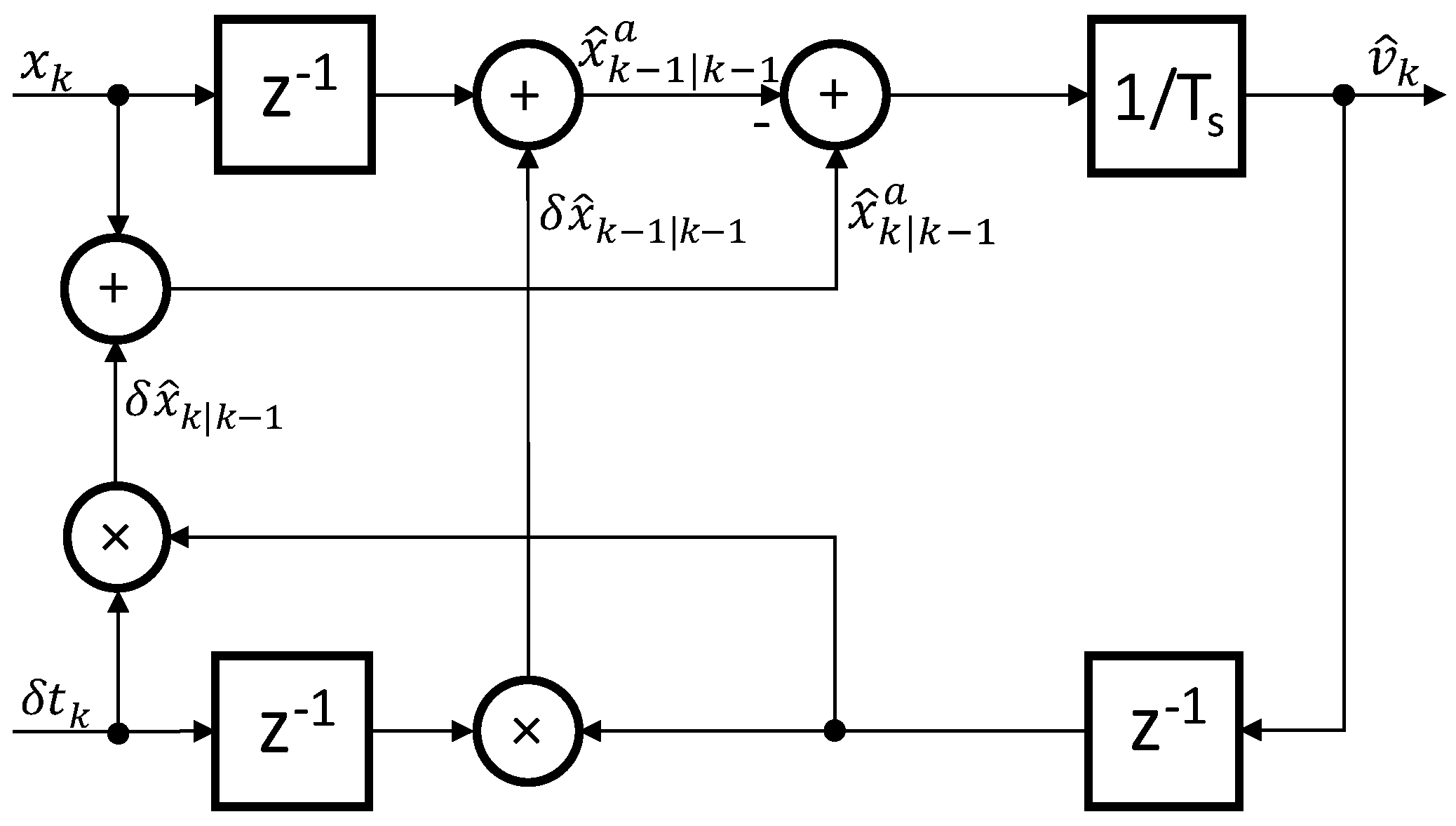
If we denote $\delta {\widehat{x}}_{k|k-1}^{}=\delta t_k{\widehat{v}}_{k-1}$ and $\delta {\widehat{x}}_{k|k}^{}=\delta t_k{\widehat{v}}_k$, then the algorithm can be presented by the block shown by Figure 6.

2.3.2. The Input–Output Dynamics

If we compare the block scheme from Figure 4 with the block scheme from Figure 6, then the higher complexity of the latter is evident. However, further analysis of the improved estimation algorithms in Equations (24)–(27) show simplification of the filter input–output structure. If we insert Equations (24) and (27) into Equation (25), then we can derive:

$${\widehat{v}}_k=\frac{{\widehat{x}}_{k|k-1}^a-{\widehat{x}}_{k-1|k-1}^a}{T_s}=\frac{(x_k+{\widehat{v}}_{k-1}\delta t_k)-(x_{k-1}^{}+{\widehat{v}}_{k-1}\delta t_{k-1})}{T_s}=\frac{\mathsf{\Delta }\delta t_k}{T_s}{\widehat{v}}_{k-1}+\frac{\mathsf{\Delta }{x}_k}{T_s}$$

(28)

where $\mathsf{\Delta }\delta t_k=\delta t_k-\delta t_{k-1}$, and $\mathsf{\Delta }{x}_k=x_k-x_{k-1}$. The latter result can be rewritten by the difference equation of the first order:

$${\widehat{v}}_k-\frac{\mathsf{\Delta }\delta t_k}{T_s}{\widehat{v}}_{k-1}=\frac{\mathsf{\Delta }{x}_k}{T_s}$$

(29)

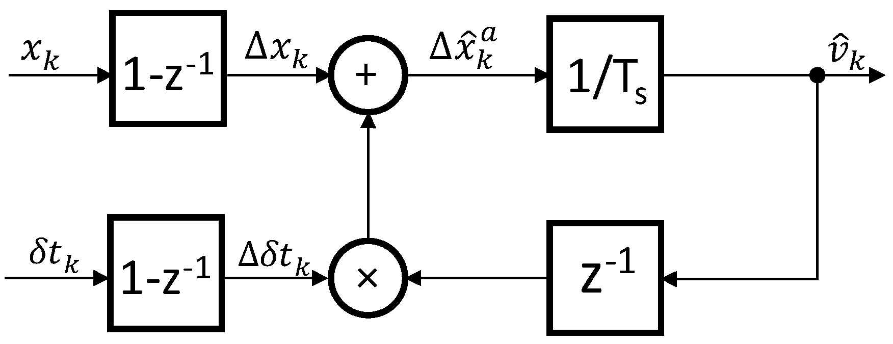
Thus, the proposed improved algorithm works as a linear time-variant filter of the first order, and is therefore called the division-less MT-type algorithm of the first order (abbreviated as the DLMT1). Accordingly, the filter structure can be described by the block scheme shown in Figure 7.

2.3.3. Stability Analysis

The stability analysis of the DLMT1 algorithm is significantly simplified in comparison with the DLMT2 algorithm. Since we assume $0\le \delta t_k<T_s$, and, thus, $-T_s<\mathsf{\Delta }\delta t_k<T_s$, then the only time variable coefficient of the linear difference in Equation (29) stays bounded, since $0\le {\tau }_k<1$ and $\left|\mathsf{\Delta }{\tau }_k\right|<1$ on bounded interval $0\le \delta t_k<T_s$ for any k > 0, where we denoted ${\tau }_k=\delta t_k/T_s$. Therefore, the stability proof is rather simple (please see the preliminaries of the stability analysis in [52]). If we introduce the auxiliary input variable $u_k=\mathsf{\Delta }{x}_k/T_s$, then the response of the linear time-variant filter of the first order (29) can be derived as a unique solution that yields:

$${\widehat{v}}_k={\mathsf{\Phi }}_k(0){\widehat{v}}_0+{\displaystyle \sum _{j=0}^{k-1}{\mathsf{\Phi }}_k(j+1)u_{j+1}}$$

(30)

where:

$${\mathsf{\Phi }}_k(j)=\{\begin{array}{cc}\mathsf{\Delta }{\tau }_k\mathsf{\Delta }{\tau }_{k-1}\dots \mathsf{\Delta }{\tau }_{j+1}& k>j\ge 0\\ 1& k=j\end{array}$$

(31)

The un-driven filter is exponentially stable if, and only if, there exists a finite positive constant γ > 0 and a constant λ with 0 ≤ λ < 1, such that [54]:

$$\left|{\mathsf{\Phi }}_k(j)\right|\le \gamma {\lambda }^{k-j},\forall k,j:k\ge j$$

(32)

The linear system under consideration is uniformly asymptotically stable if, and only if, it is uniformly exponentially stable [54]. It means that uniform exponential stability and uniform asymptotic stability are equivalent.

From the property of τ_k, we can consider that $\left|\mathsf{\Delta }{\tau }_k\right|\le \lambda <1$. Then:

$$\left|{\mathsf{\Phi }}_k(j)\right|=\left|\mathsf{\Delta }{\tau }_k\mathsf{\Delta }{\tau }_{k-1}\dots \mathsf{\Delta }{\tau }_{j+1}\right|\le \left|\mathsf{\Delta }{\tau }_k\right|\left|\mathsf{\Delta }{\tau }_{k-1}\right|\dots \left|\mathsf{\Delta }{\tau }_{j+1}\right|\le {\lambda }^{k-j},\forall k,j:k>j\ge 0$$

(33)

The latter expression proves the validity of the stability condition in Equation (32) for k > j. Furthermore, from the definition in Equation (31) follows:

$${\mathsf{\Phi }}_k(k)=1$$

(34)

which proves the existence of γ > 0 (i.e., γ = 1) and, consequently, it proves the validity of the stability condition in Equation (32) for k = j. Thus, we proved the asymptotic stability of the time-variant linear filter of the first order in Equation (29). In our case, asymptotic stability implies BIBO stability [48]. Therefore, we can simply conclude that the proposed DLMT1 algorithm is inherently asymptotically stable, and BIBO stable as well.

2.3.4. The Error Analysis

In the following, we can derive the dynamic equilibrium of the DLMT1 algorithm. If we assume ${\widehat{v}}_k={\widehat{v}}_{k-1}$ in the filter Equation (29), then it yields the equilibrium ${\widehat{v}}_k^{eq}$:

$${\widehat{v}}_k^{eq}=\frac{T_s}{T_s-\mathsf{\Delta }\delta t_k}\frac{\mathsf{\Delta }{x}_k}{T_s}=\frac{x_k-x_{k-1}}{T_s+\delta t_{k-1}-\delta t_k}$$

(35)

which equals the dynamic equilibrium of the DLMT2 method in Equation (17), and the output of the MT method in Equation (1) as well. With the definition of the convergence error as in Equation (19), we can derive its dynamics as follows. Firstly, we can derive ∆x_k from the equilibrium equation:

$$\mathsf{\Delta }{x}_k^{}=T_s{\widehat{v}}_k^{eq}-\mathsf{\Delta }\delta t_k{\widehat{v}}_k^{eq}=T_s{\widehat{v}}_k^{eq}-\mathsf{\Delta }\delta t_k({\widehat{v}}_{k-1}^{eq}+\mathsf{\Delta }{\widehat{v}}_k^{eq})$$

(36)

where $\mathsf{\Delta }{\widehat{v}}_k^{eq}={\widehat{v}}_k^{eq}-{\widehat{v}}_{k-1}^{eq}$. In the next step, we rewrite the latter equation as the difference equation of the equilibrium velocity ${\widehat{v}}_k^{eq}$:

$${\widehat{v}}_k^{eq}-\frac{\mathsf{\Delta }\delta t_k}{T_s}{\widehat{v}}_{k-1}^{eq}=\frac{\mathsf{\Delta }{x}_k^{}}{T_s}+\frac{\mathsf{\Delta }\delta t_k}{T_s}\mathsf{\Delta }{\widehat{v}}_k^{eq}$$

(37)

Then, we can subtract filter in Equation (29) from Equation (37); thus, we obtain the convergence error dynamics of the DLMT1 method:

$${\epsilon }_k^{}-\frac{\mathsf{\Delta }\delta t_k}{T_s}{\epsilon }_{k-1}^{}=\frac{\mathsf{\Delta }\delta t_k}{T_s}\mathsf{\Delta }{\widehat{v}}_k^{eq}$$

(38)

where ${\epsilon }_k$ is defined as in Equation (19). The convergence error dynamics are driven by the velocity increment $\mathsf{\Delta }{\widehat{v}}_k^{eq}$ that relates to acceleration; however, if the time interval δt_k remains constant, then the error is zeroed ${\epsilon }_k=0$, and the estimated velocity tracks its dynamic equilibrium perfectly.

We can also derive the estimation error dynamics. Following the same approach as in the previous Section 2.2, we assume that the average velocity in Equation (4) could be the best possible velocity estimation. After short manipulation, we rewrite Equation (5) as:

$${\overline{v}}_k^a-\frac{\mathsf{\Delta }\delta t_k}{T_s}{\overline{v}}_{k-1}^a=\frac{\mathsf{\Delta }{x}_k^{}}{T_s}+\frac{\delta t_k}{T_s}\mathsf{\Delta }{\overline{v}}_k^a$$

(39)

Finally, we subtract the filter Equation (29) from the latter. It yields the estimation error dynamics for the DLMT1 method:

$$e_k-\frac{\mathsf{\Delta }\delta t_k}{T_s}{e}_{k-1}=\frac{\delta t_k}{T_s}\mathsf{\Delta }{\overline{v}}_k^a$$

(40)

where $e_k$ is defined as in Equation (20). We analyze the error dynamics in the following.

The filter dynamics, and thus the error dynamics, are of the first order and asymptotically stable as well. However, similar to the case of the DLMT2 algorithm, the error is driven by the acceleration. The right hand side of Equation (40) is rather simple. If we define acceleration $a_k=\mathsf{\Delta }{\overline{v}}_k^a/T_s$, which is always bounded in practice such that $\left|a_k\right|\le a_{\max }$, then the r.h.s. expression of Equation (40) can be derived further, and its maximum absolute value can be evaluated as:

$$\left|\delta t_k{a}_k\right|\le \left|\delta t_k\right|\left|a_k\right|\le T_s\left|a_k\right|\le T_s{a}_{\max }$$

(41)

Thus, the estimation error shall not exceed $T_s{a}_{\max }$, as in the case of the MT method in Equation (12). Furthermore, it can be reduced arbitrarily by choosing a suitable short sampling period $T_s$, which is a design parameter. In the case of constant velocity, the error can converge quickly to zero.

2.4. Comparison of the Division-Less Algorithms by Numerical Examples

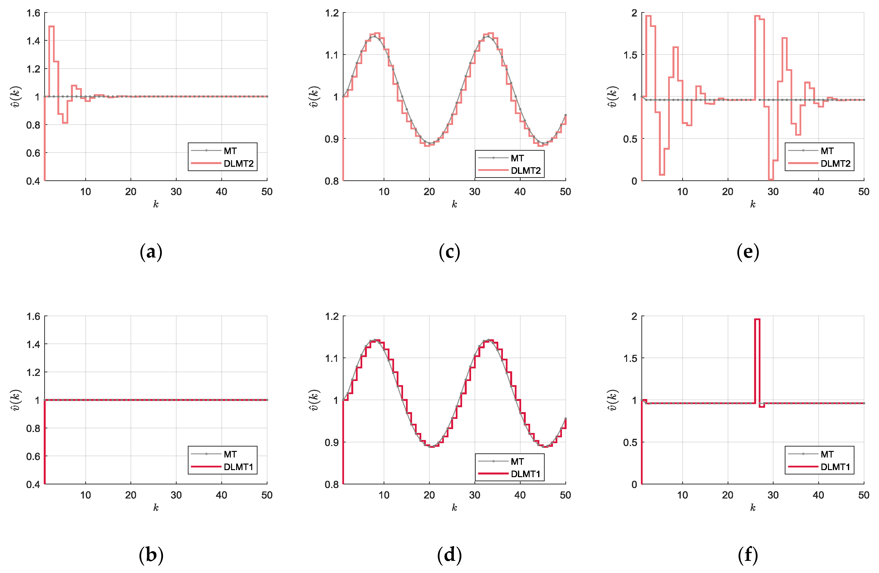
The step responses of the DLMT2 filter in Equation (16) and the novel DLMT1 filter in Equation (29), respectively, are illustrated in Figure 8. The comparison can be accomplished by the following three cases: (i) $\delta t_k/T_s$ is constant and equals 0.5, ii) $\delta t_k/T_s$ is varying by the sinus waveform of two periods with the amplitude of one and the offset of 0.5, and iii) $\delta t_k/T_s$ is varying within the interval [0, 1] by the sawtooth waveform of two periods. The dynamic equilibrium value that matches the value of the MT method estimation is also shown in the plots.

An asymptotically stable response and convergence to the dynamic equilibrium is evident in all of the cases. In the case of constant δt, we can observe an oscillatory response in the transient period for the DLMT2 algorithm, whereas a perfect response is evident for the DLMT1 algorithm. In the case of the sinusoidal variation of δt, we can observe relatively good tracking for both algorithms; however, a more smooth response with slightly better accuracy was achieved by the DLMT1 algorithm (as can be observed by comparison of Figure 8c,d. The tracking performance of the DLMT1 algorithm is better than the DLMT2 algorithm simply because the velocity error in the first case is affected by the difference Δδt only (see Equation (38)), whereas in the second case, the δt may have a significant impact as well (see Equation (18)). In the case of the sawtooth variation of δt, we can observe high-velocity peaks when the sawtooth generates abrupt changes from zero to one. Then, the DLMT2 algorithm responds with oscillatory motion, whereas the transient period produced by the DLMT1 algorithm is relatively extremely short with practically no fluctuations. However, please note that such an extreme scenario (sudden change of δt from zero to $T_s$ at the speed of 1 pp/T_s) cannot happen in practice, since it assumes momentary infinite velocity in the case when two consecutive encoder pulses become totally close together, and simultaneously stay far apart from the other pulses in the sequence. Furthermore, the MT velocity cannot be calculated in this unrealistic case, since the interpulse time interval becomes zero. However, the numerical test is still interesting, since it illustrates the characteristics of the transient response that may happen during the real operation, e.g., significant sporadic changes in δt are normal anyway, even at constant velocity, due to the asynchronous nature of the encoder pulses’ occurrences with reference to the sampling instants. We can conclude that the presented numerical cases show that the introduced DLMT1 filter performs better than the DLMT2 filter in terms of stability and accuracy.

2.5. The Experimental System

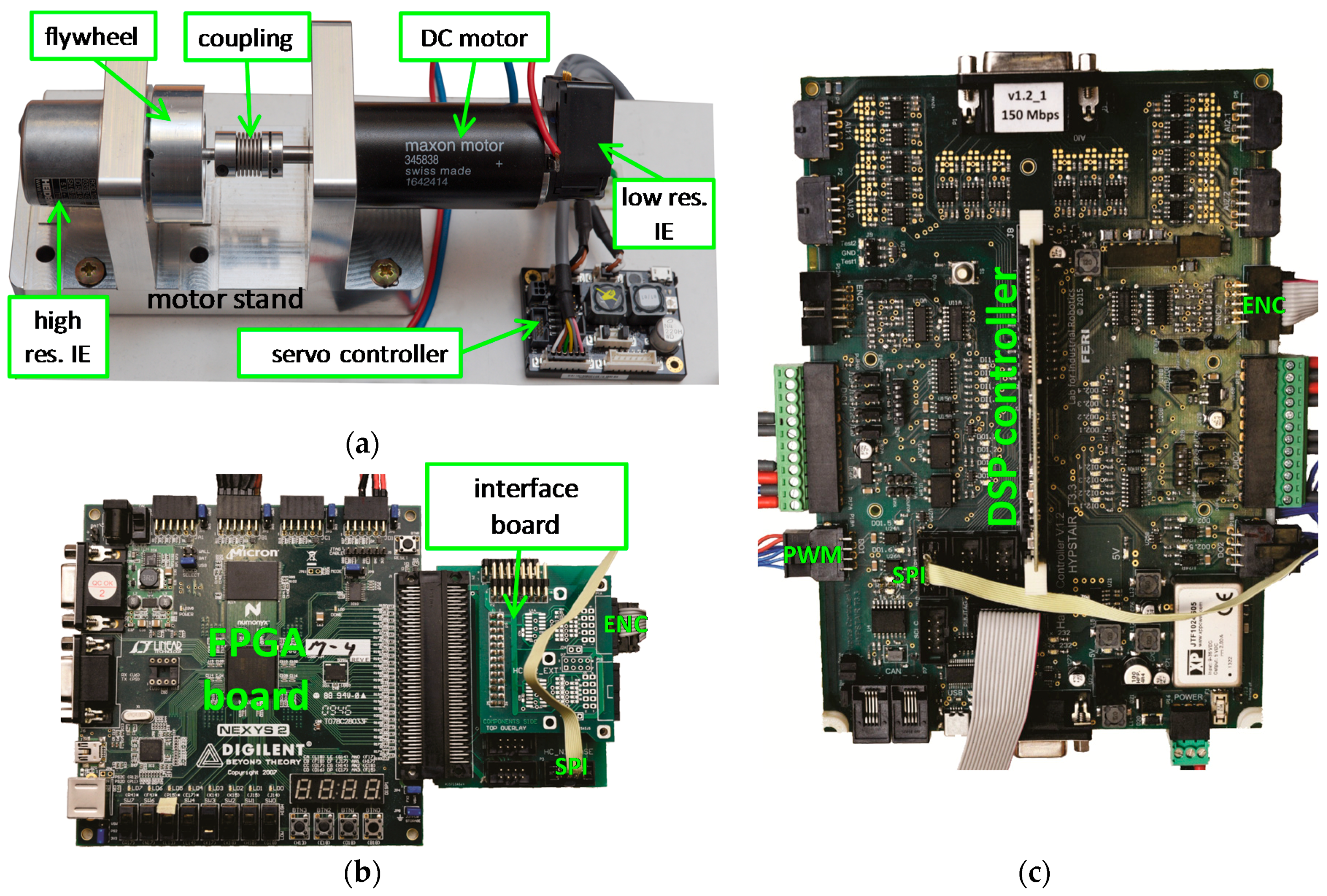
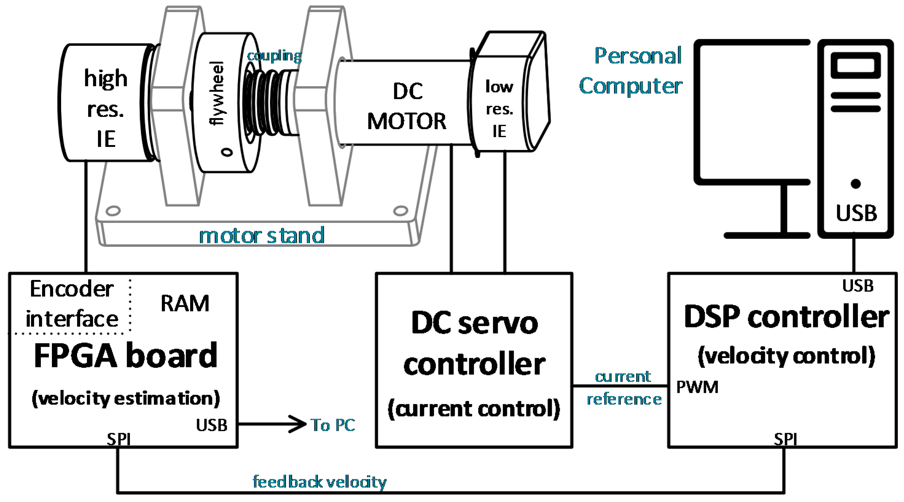
The experimental setup consists mainly of the mechanical drive system with the rotary Incremental Encoder (IE), and the processing hardware electronics. The mechanical drive system consists of a DC motor Maxon RE 35 with low-resolution Incremental Encoder HEDS 5540 (with 500 line counts per turn), mounted on the rear side of the motor shaft, and a high-resolution rotary Incremental Encoder Heidenhain ROD 1020 (with 3600 line counts per turn) is linked to the front side of the motor shaft. The latter was used for the experimental evaluation and validation of the considered methods for velocity estimation. The motor shaft and the high-resolution IE shaft are interconnected mechanically by a metal bellows coupling. Additionally, we attached a rotational flywheel on the encoder shaft, in order to reduce mechanical oscillations with increased rotational inertia. The DC motor was driven electrically by a Maxon ESCON 36/2 DC Servo Controller configured in the current control mode. The reference value for the current control loop was provided by the processor-based controller with the microcontroller TI DSP TMS320F28335, which implemented a simple velocity control loop with the PI control algorithm. The value of the control output was transferred to the Maxon servo controller via the PWM signal with the switching frequency of 5 kHz. The reference velocity was generated internally on the DSP controller, while the feedback velocity signal was provided by the testing IE, which was connected electrically to the Digilent Nexys2 FPGA board [55] via a custom interface board on the high-speed expansion connector. The interface board contains standard RS 422 line receivers, proper analog filters, and line termination. Capturing of the encoder pulses was performed by the FPGA circuit (Xilinx Spartan XC3S1200E) at 125 MHz (clock resolution of 8 ns). The sampling frequency was 10 kHz. The update of the velocity estimation output was performed synchronously with the sampling. The proposed division-less MT-type velocity estimation algorithm of the first order from Figure 7 was implemented on the FPGA board in a fixed-point format. The calculation scheme was performed by integer arithmetic operations, and executed in only a few FPGA clock cycles (less than 100 ns) with minimal resource consumption. The data required for the velocity control loop were transmitted to the DSP controller via SPI communication in real time in every sampling period. These data were the estimation values for the feedback velocity obtained by the proposed algorithm implemented on the FPGA board, and the other data required for velocity estimation by other algorithms and methods for comparison purpose. The online computation on the DSP controller was performed in real time in single precision floating-point format. The bidirectional full-duplex SPI communication enabled the data transfer from the DSP controller on the FPGA board simultaneously. The data were logged in the RAM on the FPGA board in real time, in order to be transferred later to the desktop computer for offline post-processing. The desktop computer was connected to the FPGA board by a USB communication link. We performed data post-processing offline in double precision floating-point format. Some more detailed information of the experimental system can be found in [53]. However, one should note that the current experimental system is an upgraded version of the previous one, with the following main differences. (a) We replaced the DC motor with a larger version in order to reduce mechanical oscillations. (b) The servo controller was configured in the current control mode. (c) We added the DSP controller, which performed the velocity control loop and other computations (the reference trajectory and alternative velocity estimation algorithms for comparison purposes). (d) The FPGA implemented the proposed division-less algorithm of the first order. The main components of the system are shown by Figure 9, whereas the experimental system scheme is presented by Figure 10.

3. Results

The proposed division-less MT-type methods for velocity estimation may show instability in practical implementation when blank sampling intervals appear at low speed. The problem is discussed well in [53], where the basic DLMT2 algorithm has been properly adapted in order to guarantee stability in a wide-speed range operation. Thus, such a generalized version of the algorithm is abbreviated as GDLMT2. Similarly, the basic DLMT1 algorithm must be generalized for stable practical operation as well. In this paper, we adopt the same approach as that introduced in [53]. Then, the adapted version is denoted as GDLMT1.

Based on the experience in [53], we firstly performed experiments such that we decoupled the testing IE with the flywheel from the motor shaft mechanically. Thus, we could remove the mechanical noise from the IE rotation as much as possible. Namely, the induced mechanical noise may blur the tested method’s performance. However, in the case of a manually driven IE (i.e., driving the encoder flywheel by hand), we could not control the velocity profile, and the achieved maximum speed was quite limited. Thus, we continued performing experiments with the IE coupled on the motor shaft. In this case, the IE was involved in the control loop, providing velocity feedback for the motor control. These experiments validated the proposed velocity estimation algorithm for the motion control applications.

We performed numerous experiments with the manually driven IE (so-called manual experiments) and motor driven IE (so-called motorized experiments). We recorded the raw sampled data from the IE and the computed velocity in real time on the FPGA board (GDLMT1 method) and the DSP controller (MT method). The recorded raw sampled data enabled us to calculate the velocity on the desktop computer in offline post-processing mode using the MATLAB software package. Thus, we could compare the performance of the proposed algorithm with other algorithms. We also involved the filtered M method with the Butterworth filter of the second order, which is a very common method for velocity estimation in less demanding motion control applications. However, we assumed that the original MT method can be considered as the reference method; thus, we compared the division-less algorithms with that one. The diagrams below showing experimental results typically involve traces, which denote: (i) the sampled encoder pulses in a single sampling period (so-called encoder velocity) that is equivalent to the basic M method (light green solid line trace), (ii) the velocity computed by the MT method on the DSP controller in real time (dark red solid line trace with squares), (iii) the velocity computed by the fixed-point GDLMT1 algorithm on the FPGA in real time (pink solid line trace with diamonds), (iv) the velocity computed offline by the floating-point GDLMT1 algorithm on the desktop computer (red solid line trace with stars), (v) the velocity computed offline by the floating-point GDLMT2 algorithm on the desktop computer (light red solid line trace with circles), (vi)–(vii) the velocity obtained by Butterworth filtering with the cut-off frequencies of 100 Hz (dark green solid line trace with dots) and 50 Hz (green dash dot line trace), respectively. Additionally, in the manual experiments, we show the so-called “actual” velocity, whereas in the motorized experiments, we show the reference velocity (blue dashed line trace in both cases). The “actual” velocity was obtained offline by a non-causal discrete zero-phase low-pass Butterworth filter with a cut-off frequency of 50 Hz, whereas the reference velocity was computed on the DSP controller in real time. The velocity is given in units of “position pulses per sampling period” (pp/T_s).

3.1. The Manual Experiments

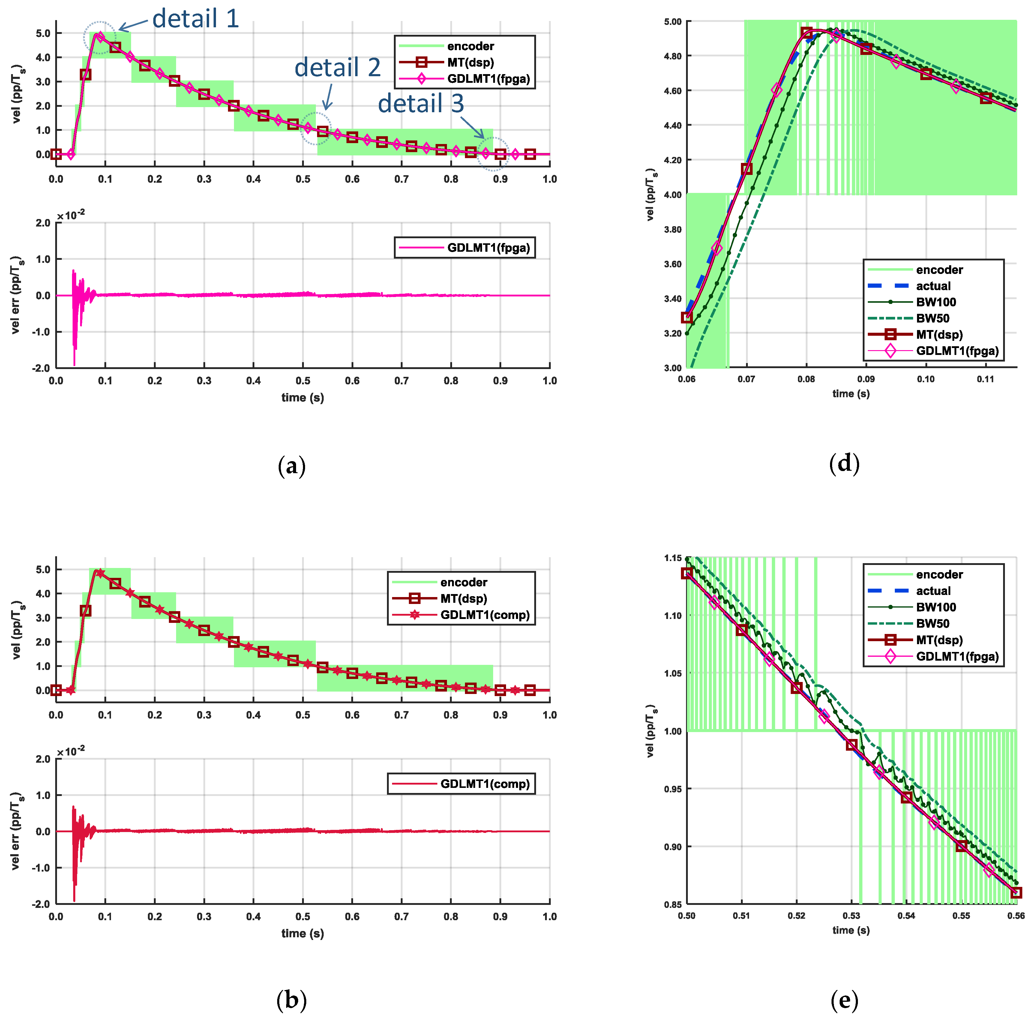
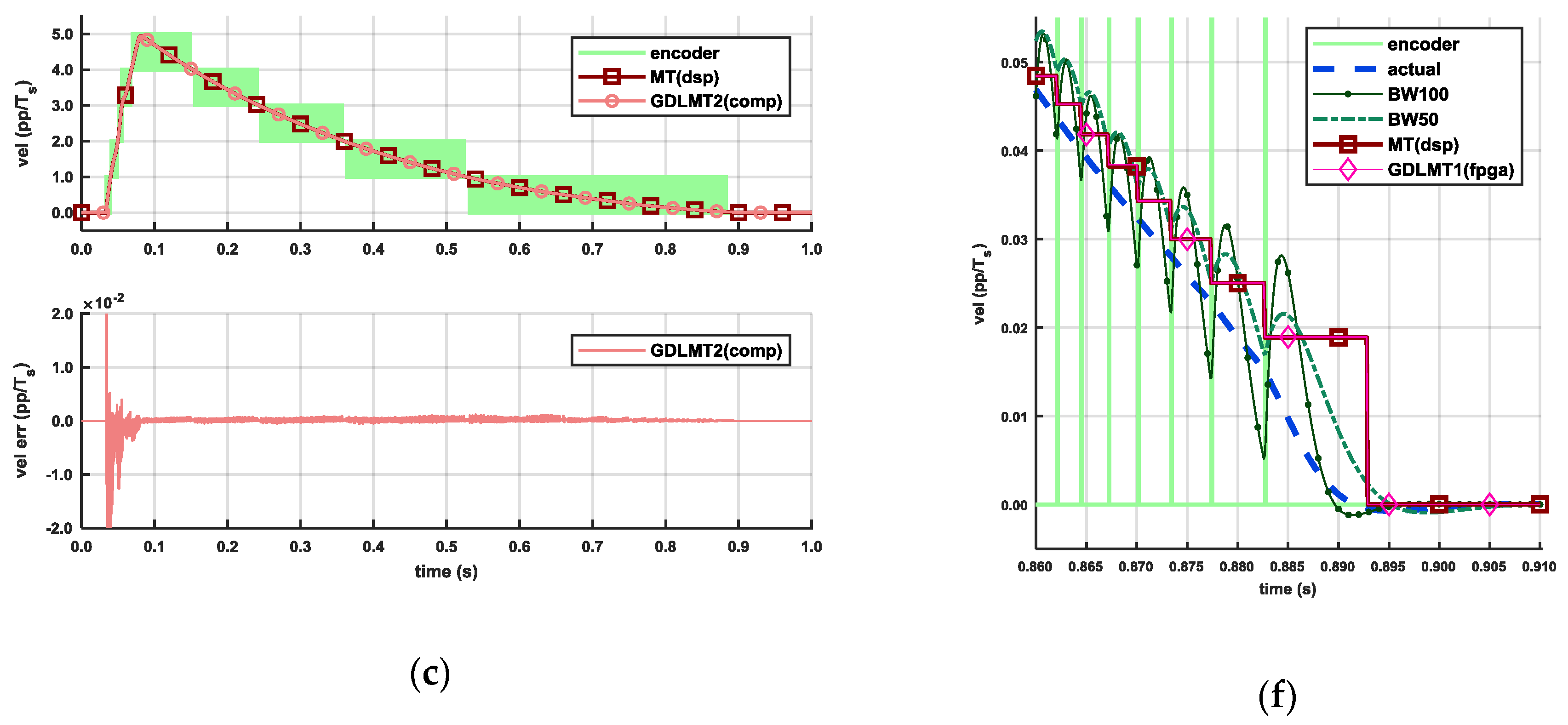
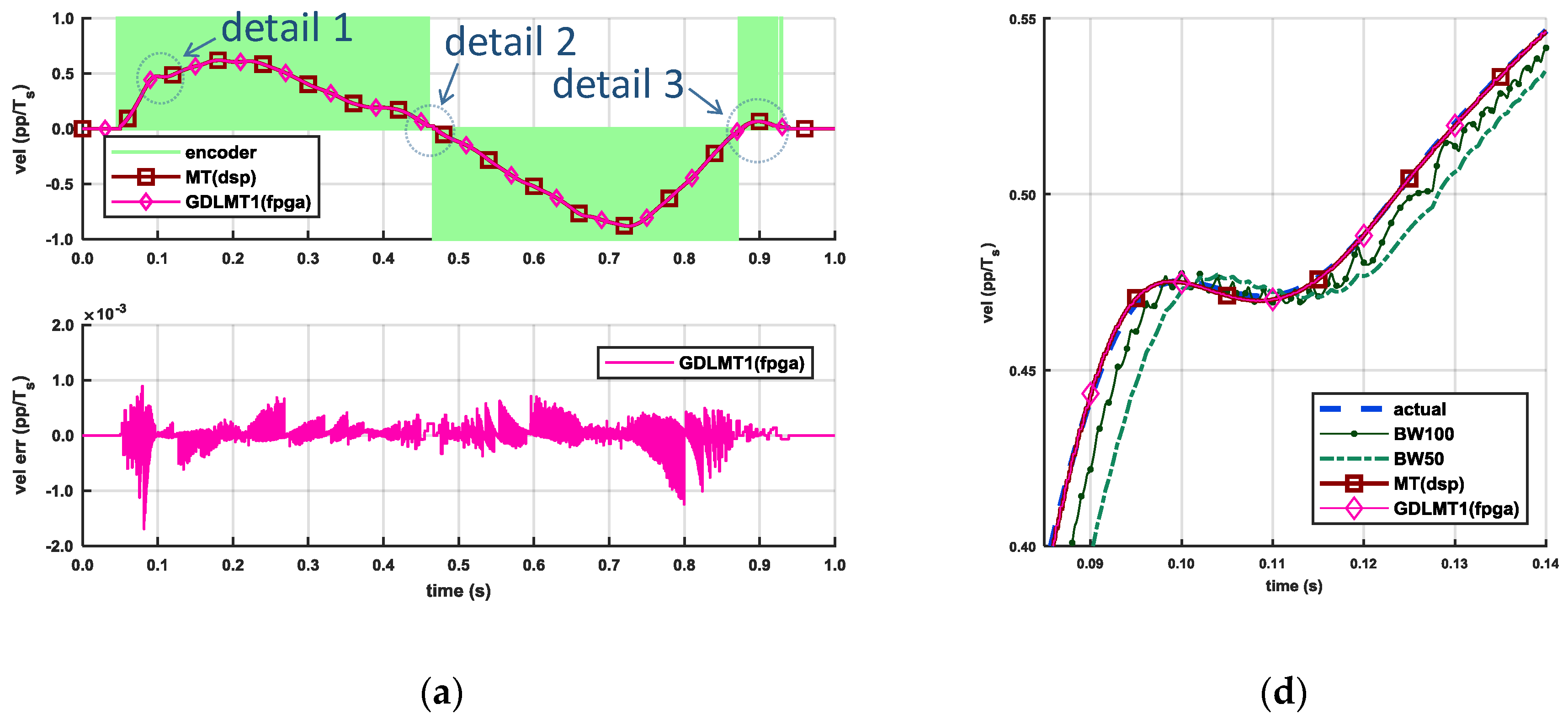
Figure 11 shows the results from manual experiment number one. In this experiment, we pushed the encoder flywheel by hand strongly, and then left it to stop gradually by itself. Thus, we achieved smooth motion with the velocity peak close to 5 pp/T_s. The upper plots on the diagrams in Figure 11a–c show: (i) the encoder velocity, (ii) the MT velocity computed on the DSP controller in real time, and (iii) the velocity obtained by one of the division-less MT-type algorithms, i.e., (a) the fixed-point GDLMT1 algorithm on the FPGA, (b) the floating-point GDLMT1 algorithm on the offline computer, or (c) the floating-point GDLMT2 algorithm on the offline computer. The bottom plots on the diagrams Figure 11a–c show the corresponding velocity error with reference to the MT velocity. The velocity plots demonstrate smooth traces of the MT-type methods that match almost perfectly. The error plots further confirm that they match well, since the velocity error stays very low, i.e., below 0.02 pp/T_s. However, it is evident that the error peaks in the GDLMT2 method exceed that limit. The error increased during the high acceleration phase at the start; however, it practically disappeared after the velocity peak. The plots on Figure 11a,b also show clearly that the error traces of both the GDLMT1 implementations are almost identical. This verifies the fixed-point implementation on the FPGA. If we compare the error plot on Figure 11c with the corresponding error plot on Figure 11a or Figure 11b, then we can observe a slightly larger error in the case of the GDLMT2 method in the whole time interval. The next plots on Figure 11d,f show some interesting details from the velocity plot shown in diagram Figure 11a. (i) Detail 1 focuses on the velocity peak, (ii) Detail 2 focuses on the crossing to the velocity below 1 pp/T_s, when blank sampling intervals start to appear, and (iii) Detail 3 focuses on the final stop phase. The details show the encoder velocity, the MT velocity, and the GDLMT1 velocity, respectively, although we added some more velocity traces for the comparison: the “actual” velocity and the velocities obtained by Butterworth filtering with 100 Hz (abbreviated as BW100) and 50 Hz (abbreviated as BW50), respectively. The plot in Figure 11d shows smooth velocity traces in all cases, the MT-type velocities match well with the “actual” velocity, while the BW100 and BW50 traces show a significant phase lag as expected, respectively. The plot in Figure 11e shows very similar performance for the MT-type velocity traces; however, the BW100 velocity trace fluctuates synchronously with the alternation of the encoder velocity. A relatively large fluctuation of the BW100 velocity trace can also be observed on plot Figure 11f. In this case, the BW50 velocity trace fluctuates as well, although to a lesser degree. This phenomenon is due to the sensitivity of the filter on the individual input pulses generated by the encoder at low speed. These rare encoder pulses, on the other hand, cause the stair-like MT-type velocity traces, which match perfectly. However, a delay with reference to the “actual” velocity is evident as well. This is because the MT method updates only if at least one encoder pulse occurs, and, in this case, it can only calculate an average velocity in the recent interpulse time interval (i.e., the time interval between two adjacent encoder pulses). If the interpulse interval is relatively long, then a significant error with reference to the actual velocity at the current sampling instant can appear in the case of accelerated or decelerated motion. When motion stops, the encoder pulses disappear as well, and the MT method cannot update the velocity. In order to deal with this problem, we simply zeroed the velocity after a predefined time interval elapsed (i.e., 10 ms). In order to provide a more accurate estimation in this case, the approach such as in [56] can be adopted; however, this is out of the scope of this paper.

In manual experiment number two, we performed sinusoidal motion at relatively low speed. In this case, the velocity did not exceed 1 pp/T_s. The results are depicted by Figure 12, which is organized similarly to Figure 11. We can also make very similar observations for the diagrams in Figure 12a–c. Some interesting details from the diagram Figure 12a are depicted by the diagrams in Figure 12d–f, which focus on the saddle point (d), the zero-crossing (e), and the stop with overshoot (f). Diagram Figure 12d shows smooth velocity traces for the MT method and the GDLMT1 method, respectively, which both match the “actual” velocity almost perfectly. The BW50 velocity trace is quite smooth as well; however, the BW100 velocity trace shows fluctuation. Such fluctuation is even more expressed on diagrams Figure 12e,f. Here, we can observe the stair-like velocity traces of the MT-type methods, which appear due to rare encoder pulses and blank sampling intervals. Matching the GDLMT1 velocity trace with the MT velocity trace is evident, whereas the lag with reference to the “actual” velocity due to the averaging velocity of the recent past interpulse interval can also be observed clearly.

3.2. The Motorized Experiments

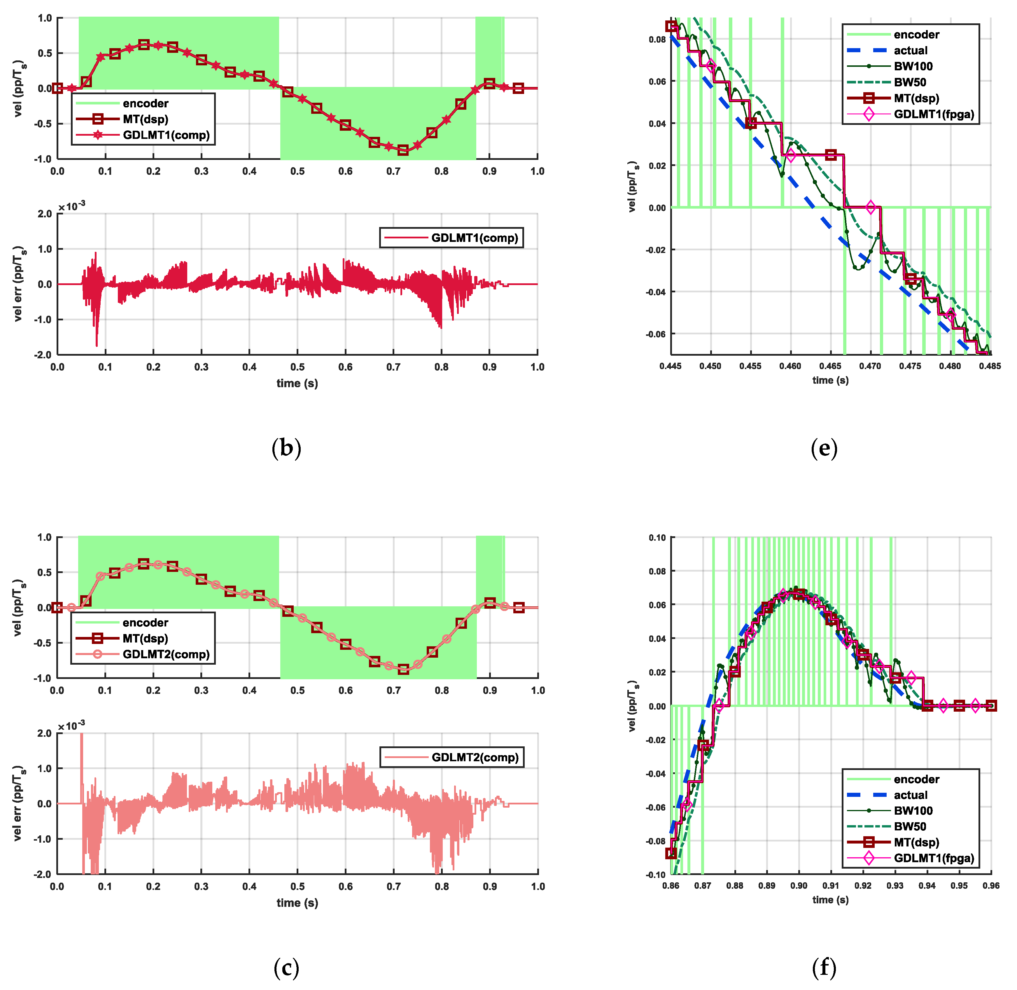
Figure 13 illustrates the experimental results with the trapezoidal velocity profile of relatively high set point speed (10 pp/T_s), which were obtained by the motor-driven configuration. The servo drive system was configured in velocity closed-loop control with the testing IE for velocity feedback. Diagram Figure 13a depicts the results with the GDLMT1 algorithm implemented on the FPGA, whereas diagram Figure 13b depicts the results with the MT velocity computed on the DSP. The upper plots show the encoder velocity, the reference velocity, and the feedback velocity. Both plots demonstrate good matching of the feedback velocity with the reference velocity. The middle plots show the control error, i.e., the difference between the reference velocity and the feedback velocity. The control errors are almost the same. The bottom plot in diagram Figure 13a shows the velocity error of the used feedback velocity, i.e., obtained by the GDLMT1 algorithm on the FPGA, and the plot in diagram Figure 13b shows the velocity error of the GDLMT2 velocity computed offline. By comparison of these plots, we can observe a larger error in the case of the GDLMT2 velocity. Diagrams Figure 13c,d show details 1 and 2, respectively, from diagram Figure 13a. Detail 1 illustrates the overshoot of when the actual velocity converged to the set point speed, whereas detail 2 focuses on the traveling phase. We can record an overshoot of 0.1 pp/T_s, pretty smooth velocity in the transient phase, a small ripple of magnitude of 0.005 pp/T_s in the case of the GDMLT1 velocity due to the mechanical noise, and larger fluctuation of the velocity obtained by the filtering method (at BW50, and even more distinctive at BW100) caused by alternation of the encoder pulses.

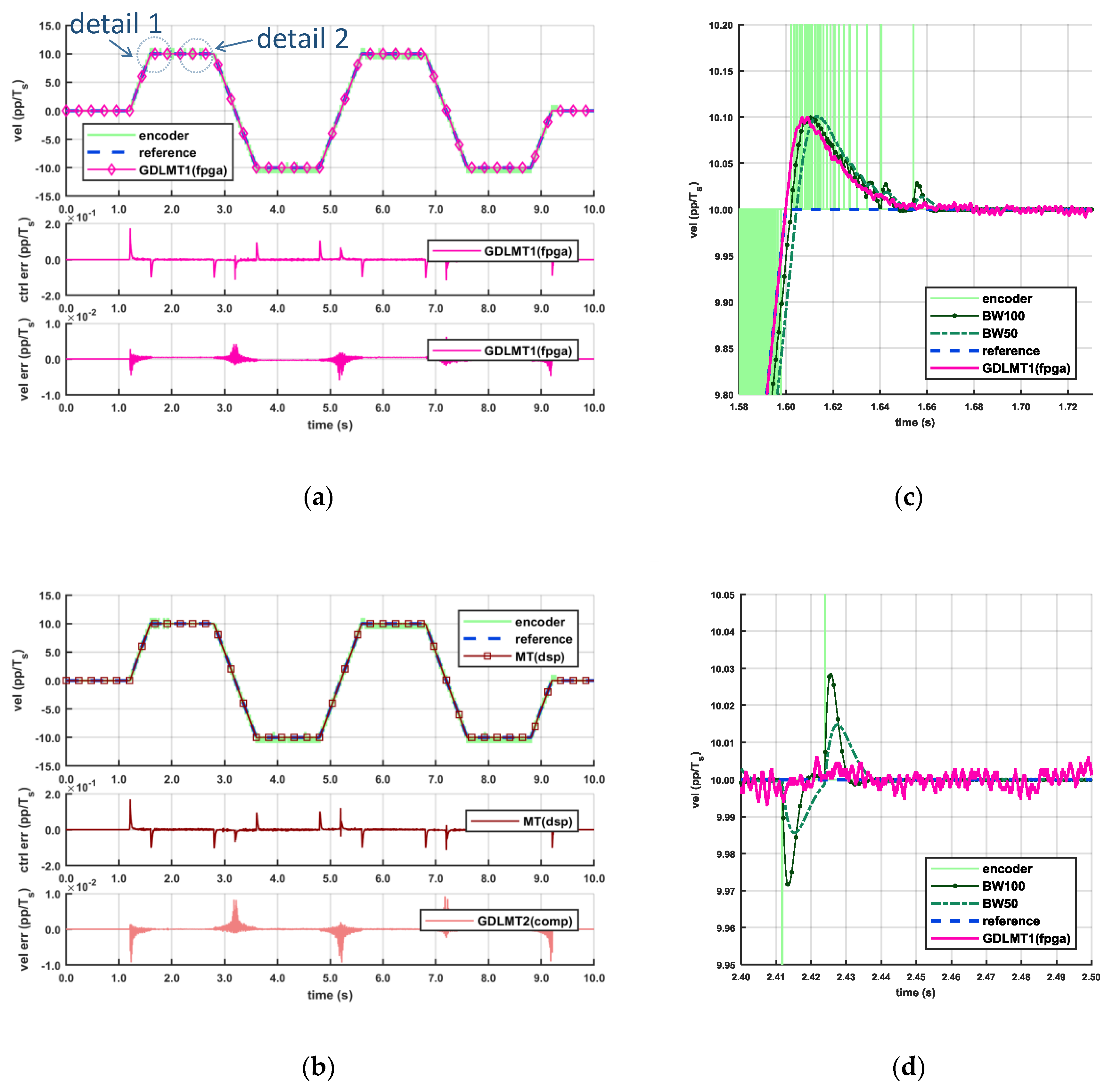
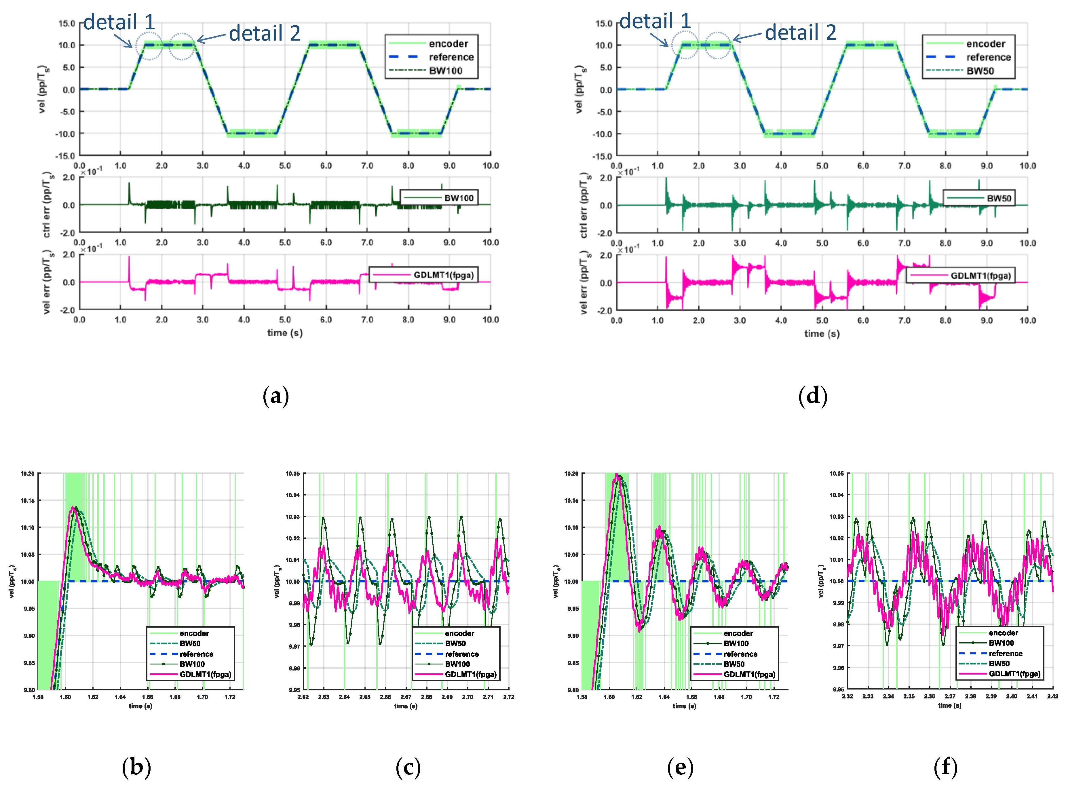
We then repeated the experiment; however, we changed the feedback velocity. Instead of the MT-type velocity, we applied the velocity signal obtained by the Butterworth filter (the filtered M method velocity). The control loop remained tuned as it was in Figure 13. The results are depicted by Figure 14: diagrams (a)–(c) show the case with the BW100 velocity, whereas diagrams (d)–(f) show the case with the BW50 velocity. More specifically, diagrams Figure 14a,d depict the reference velocity profile, along with the encoder velocity and the feedback velocity on the upper plots, the control error on the middle plots, and the difference between the reference velocity and the GDLMT1 velocity on the bottom plots. The “big picture” illustrated by the upper plots hides the details; however, it is easy to observe the permanent noise of the encoder velocity. The control error reveals a relatively high ripple in the case of the BW100 velocity, which is also demonstrated on the GDLMT1 velocity error on the plot below. In the case of the BW50 velocity, one can see more oscillations in the transient phase. Details 1 and 2 from diagram Figure 14a are illustrated by the plots Figure 14b,c, respectively. The overshoot of ca. 0.14 pp/T_s can be noted in Figure 14a, which is 40% more than in the case with the GDLMT1 feedback velocity in Figure 13c. Furthermore, a large ripple is evident, not only in the BW100 velocity, but also in the GDLMT1 velocity. If we consider that the GDLMT1 velocity is close to the actual velocity, then we can deduce that this could be the true velocity. Thus, the ripple is caused by the BW100 velocity used in the feedback control. Details 1 and 2 from diagram Figure 14d that are shown in the plots Figure 14e,f somehow confirm the observations from the “big picture” for the BW50 velocity case, which include: i) relatively large oscillations in the transient phase with an overshoot of ca. 0.20 pp/T_s (100% more than in the case with the GDLMT1 feedback velocity), which relates to lower stability of the control loop (a result of a worse phase margin due to the lower cut-off frequency), and ii) a large ripple during the traveling phase. Thus, although the BW50 velocity was smoother than the BW100 velocity, its application in the feedback deteriorated the system output response further.

4. Discussion

As shown in the previous section, we performed a large number of experiments. The experiments verified clearly the FPGA implementation of the proposed division-less MT-type algorithm of the first order (DLMT1). The velocity estimation obtained by the FPGA was matched with the results obtained offline on the post-processing computer utilizing the floating-point arithmetic in the double-precision mode. The generalized version of the DLMT1 method provides accurate velocity estimation in a wide range, which is comparable with the conventional MT method. Furthermore, the experimental comparison analysis also showed that the proposed simplified DLMT1 method outperformed the DLMT2 method in terms of the velocity error, which was reduced by approximately 40%. When we applied the proposed division-less algorithm in the control loop, it provided practically the same control performance as the original MT method, which was implemented on the powerful DSP controller by floating point arithmetic in single precision. If we compare the application of the MT-type velocities (including the GDLMT1 velocity) in the control loop with the filtered M method (BW50, BW100), then the former enables better overall control performance, including lower control error, lower overshoot, and significantly less ripple in the control output response. We can sum up that the proposed MT-type division-less algorithm, along with its FPGA implementation, was validated experimentally for motion control applications.

5. Conclusions

In this paper, we redesigned the computation algorithm of velocity estimation of the well-known MT method for Incremental Encoders. In our approach, we replaced the arithmetical division that is inherent to the conventional MT method calculus by simpler arithmetic operations, such as multiplication and addition. This yields a division-less MT-type algorithm. This simplification enables the implementation of the MT-type algorithm on low-cost FPGAs. However, the algorithm is recursive, and described as a time-variant discrete filter. The original proposal has been determined by the second-order system, which, under some conditions, could generate weakly damped responses with undesired fluctuations during the transient phase. We focused on order reduction, and thus modified the original algorithm such that we derived the recursive algorithm of the first order, which represents the main novelty of the paper. The stability and convergence of the proposed algorithm was discussed theoretically and proven properly. The numerical examples are also shown in the paper; they demonstrate significant improvement in the transient phase of the filter step response. The novel algorithm was also validated experimentally. It was implemented on the experimental FPGA board, and tested by the industrial rotary Incremental Encoder. The algorithm implementation occupied only a few FPGA resources, which qualifies it for modern small size cost-optimized FPGAs. Furthermore, the execution time is negligible for motion control applications. The real-time experiments demonstrated smooth and highly accurate velocity estimation. The obtained experimental results were compared with other methods. The comparison showed excellent matching with the conventional MT method, and lower velocity error in comparison with the division-less MT-type algorithm of the second order. Therefore, the performance improvement was confirmed by practical experiments. Further experimental validation focused on the application of the novel algorithm for velocity feedback in a simple closed-loop control system with a DC servo motor. The proposed method provided similar control performance as the original MT method. Furthermore, it clearly outperformed the filtered M method in terms of smoothness, phase lag, and transient response of the closed-loop control. Thus, the proposed division-less MT-type velocity estimation algorithm for low-cost FPGAs was validated for motion control applications.

References

- Monmasson, E.; Idkhajine, L.; Cirstea, M.N.; Bahri, I.; Tisan, A.; Naouar, M.W. FPGAs in industrial control applications. IEEE Trans. Ind. Inform. 2011, 7, 224–243. [Google Scholar] [CrossRef]
- Rodríguez-Andina, J.J.; Valdés-Peña, M.D.; Moure, M.J. Advanced features and industrial applications of FPGAs—A review. IEEE Trans. Ind. Inform. 2015, 11, 853–864. [Google Scholar] [CrossRef]
- De la Piedra, A.; Braeken, A.; Touhafi, A. Sensor systems based on FPGAs and their applications: A survey. Sensors 2012, 12, 12235–12264. [Google Scholar] [CrossRef]
- García, G.J.; Jara, C.A.; Pomares, J.; Alabdo, A.; Poggi, L.M.; Torres, F. A survey on FPGA-based sensor systems: Towards intelligent and reconfigurable low-power sensors for computer vision, control and signal processing. Sensors 2014, 14, 6247–6278. [Google Scholar] [CrossRef] [PubMed]
- Jhang, J.-Y.; Tang, K.-H.; Huang, C.-K.; Lin, C.-J.; Young, K.-Y. FPGA implementation of a functional neuro-fuzzy network for nonlinear system control. Electronics 2018, 7, 145. [Google Scholar] [CrossRef]
- Ricci, S.; Meacci, V. Simple torque control method for hybrid stepper motors implemented in FPGA. Electronics 2018, 7, 242. [Google Scholar] [CrossRef]
- Hace, A.; Franc, M. FPGA implementation of sliding-mode-control algorithm for scaled bilateral teleoperation. IEEE Trans. Ind. Inform. 2013, 9, 1291–1300. [Google Scholar] [CrossRef]
- Hace, A.; Franc, M. Pseudo-sensorless high-performance bilateral teleoperation by sliding-mode control and FPGA. IEEE/ASME Trans. Mechatron. 2014, 19, 384–393. [Google Scholar] [CrossRef]
- Martínez-Prado, M.; Rodríguez-Reséndiz, J.; Gómez-Loenzo, R.; Herrera-Ruiz, G.; Franco-Gasca, L. An FPGA-based open architecture industrial robot controller. IEEE Access 2018, 6, 13407–13417. [Google Scholar] [CrossRef]
- Zhu, W.-H.; Lamarche, T.; Dupuis, E.; Jameux, D.; Barnard, P.; Liu, G. Precision control of modular robot manipulators: The vdc approach with embedded FPGA. IEEE Trans. Robot. 2013, 29, 1162–1179. [Google Scholar] [CrossRef]
- Cerezo, J.O.; Morales, E.C.; Plaza, J.M.C. Control system in open-source FPGA for a self-balancing robot. Electronics 2019, 8, 198. [Google Scholar] [CrossRef]
- Singh, S.; Shekhar, C.; Vohra, A. FPGA-based real-time motion detection for automated video surveillance systems. Electronics 2016, 5, 10. [Google Scholar] [CrossRef]
- Giaconia, G.C.; Greco, G.; Mistretta, L.; Rizzo, R. Exploring FPGA-based lock-in techniques for brain monitoring applications. Electronics 2017, 6, 18. [Google Scholar] [CrossRef]
- Bravo-Muñoz, I.; Lázaro-Galilea, J.L.; Gardel-Vicente, A. FPGA and soc devices applied to new trends in image/video and signal processing fields. Electronics 2017, 6, 25. [Google Scholar] [CrossRef]
- Lopes Ferreira, M.; Canas Ferreira, J. An FPGA-oriented baseband modulator architecture for 4g/5g communication scenarios. Electronics 2019, 8, 2. [Google Scholar] [CrossRef]
- Lygouras, J.N.; Kodogiannis, V.; Pachidis, T.P.; Sirakoulis, G.C. A new method for digital encoder adaptive velocity/acceleration evaluation using a TDC with picosecond accuracy. Microprocess. Microsyst. 2009, 33, 453–460. [Google Scholar] [CrossRef]
- Abbaszadeh, A.; Iakymchuk, T.; Bataller-Mompeán, M.; Francés-Villora, J.V.; Rosado-Muñoz, A. Anscalable matrix computing unit architecture for FPGA, and SCUMO user design interface. Electronics 2019, 8, 94. [Google Scholar] [CrossRef]
- Liu, Z.; Chow, P.; Xu, J.; Jiang, J.; Dou, Y.; Zhou, J. A uniform architecture design for accelerating 2D and 3D CNNS on FPGAs. Electronics 2019, 8, 65. [Google Scholar] [CrossRef]
- Ice40 Ultraplus™ Family—Data Sheet; Lattice Semiconductor: Portland, OR, USA, 2017.
- Rodríguez Andina, J.J.; de la Torre Arnanz, E.; Valdés Peña, M.D. FPGAs—Fundamentals, Advanced Features and Applications in Industrial Electronics; CRC Press: Boca Raton, FL, USA, 2017. [Google Scholar]
- Bourogaoui, M.; Ben Attia Sethom, H.; Slama Belkhodja, I. Speed/position sensor fault tolerant control in adjustable speed drives—A review. ISA Trans. 2016, 64, 269–284. [Google Scholar] [CrossRef] [PubMed]
- Kennel, R.M. Why do incremental encoders do a reasonably good job in electrical drives with digital control? In Proceedings of the Conference Record of the 2006 IEEE Industry Applications Conference Forty-First IAS Annual Meeting, Tampa, FL, USA, 8–12 October 2006; pp. 925–930. [Google Scholar]
- Kennel, R.M. Encoders for simultaneous sensing of position and speed in electrical drives with digital control. In Proceedings of the Fortieth IAS Annual Meeting—Conference Record of the 2005 Industry Applications Conference, Kowloon, Hong Kong, China, 2–6 October 2005; pp. 731–736. [Google Scholar]
- Ohnishi, K.; Shibata, M.; Murakami, T. Motion control for advanced mechatronics. IEEE/ASME Trans. Mechatron. 1996, 1, 56–67. [Google Scholar] [CrossRef]
- Tsuji, T.; Hashimoto, T.; Kobayashi, H.; Mariko, M.; Ohnishi, K. A wide-range velocity measurement method for motion control. IEEE Trans. Ind. Electron. 2009, 56, 510–519. [Google Scholar] [CrossRef]
- Kavanagh, R.C. Performance analysis and compensation of m/t-type digital tachometers. IEEE Trans. Instrum. Meas. 2001, 50, 965–970. [Google Scholar] [CrossRef]
- Petrella, R.; Tursini, M.; Peretti, L.; Zigliotto, M. Speed measurement algorithms for low-resolution incremental encoder equipped drives: A comparative analysis. In Proceedings of the 2007 International Aegean Conference on Electrical Machines and Power Electronics, Bodrum, Turkey, 10–12 September 2007; pp. 780–787. [Google Scholar]
- Puglisi, L.J.; Saltaren Pazmiño, R.J.; García Cena, C.E. On the velocity and acceleration estimation from discrete time-position sensors. J. Control Eng. Appl. Inform. 2015, 17, 30–40. [Google Scholar]
- Carneiro, J.F.; De Almeida, F.G. On the influence of velocity and acceleration estimators on a servopneumatic system behaviour. IEEE Access 2016, 4, 6541–6553. [Google Scholar] [CrossRef]
- Chawda, V.; Celik, O.; O’Malley, M.K. Evaluation of velocity estimation methods based on their effect on haptic device performance. IEEE/ASME Trans. Mechatron. 2018, 23, 604–613. [Google Scholar] [CrossRef]
- Kim, J.; Kim, B.K. Development of precise encoder edge-based state estimation for motors. IEEE Trans. Ind. Electron. 2016, 63, 3648–3655. [Google Scholar] [CrossRef]
- Gutiérrez-Giles, A.; Arteaga-Pérez, M.A. GPI based velocity/force observer design for robot manipulators. ISA Trans. 2014, 53, 929–938. [Google Scholar] [CrossRef] [PubMed]
- Saudabayev, A.; Varol, H.A. Sensors for robotic hands: A survey of state of the art. IEEE Access 2015, 3, 1765–1782. [Google Scholar] [CrossRef]
- Kirchhoff, J.; von Stryk, O. Velocity estimation for ultralightweight tendon-driven series elastic robots. IEEE Robot. Autom. Lett. 2018, 3, 664–671. [Google Scholar] [CrossRef]
- Aguado-Rojas, M.; Pasillas-Lépine, W.; Loría, A.; De Bernardinis, A. Angular velocity estimation from incremental encoder measurements in the presence of sensor imperfections. IFAC-PapersOnline 2017, 50, 5979–5984. [Google Scholar] [CrossRef]
- Bascetta, L.; Magnani, G.; Rocco, P. Velocity estimation: Assessing the performance of non-model-based techniques. IEEE Trans. Control Syst. Technol. 2009, 17, 424–433. [Google Scholar] [CrossRef]
- Ohmae, T.; Matsuda, T.; Kamiyama, K.; Tachikawa, M. A microprocessor-controlled high-accuracy wide-range speed regulator for motor drives. IEEE Trans. Ind. Electron. 1982, IE-29, 207–211. [Google Scholar] [CrossRef]
- Prokin, M. Extremely wide-range speed measurement using a double-buffered method. IEEE Trans. Ind. Elecron. 1994, 41, 550–559. [Google Scholar] [CrossRef]
- Kavanagh, R.C. An enhanced constant sample-time digital tachometer through oversampling. Trans. Inst. Meas. Control 2004, 26, 83–98. [Google Scholar] [CrossRef]
- Pu, J.-T.; Wang, H. A novel variable m/t method for speed measurement with high precision. In Proceedings of the 2nd International Conference on Electronic & Mechanical Engineering and Information Technology (EMEIT-2012), Shenyang, China, 7–9 December 2012; Atlantis Press: Paris, France, 2019; pp. 1855–1858. [Google Scholar]
- Hachiya, K.; Ohmae, T. Digital speed control system for a motor using two speed detection methods of an incremental encoder. In Proceedings of the 2007 European Conference on Power Electronics and Applications, Aalborg, Denmark, 2–5 September 2007; pp. 1–10. [Google Scholar]
- Chen, Y.; Yang, M.; Long, J.; Xu, D.; Blaabjerg, F. M/t method based incremental encoder velocity measurement error analysis and self-adaptive error elimination algorithm. In Proceedings of the IECON 2017—43rd Annual Conference of the IEEE Industrial Electronics Society, Beijing, China, 29 October–1 November 2017; pp. 2085–2090. [Google Scholar]
- Merry, R.J.; van de Molengraft, R.; Steinbuch, M. Error modeling and improved position estimation for optical incremental encoders by means of time stamping. In Proceedings of the 2007 American Control Conference, New York, NY, USA, 9–13 July 2007; pp. 3570–3575. [Google Scholar]
- Merry, R.J.; van de Molengraft, M.J.; Steinbuch, M. Velocity and acceleration estimation for optical incremental encoders. Mechatronics 2010, 20, 20–26. [Google Scholar] [CrossRef] [Green Version]
- Kavanagh, R.C. Improved digital tachometer with reduced sensitivity to sensor nonideality. IEEE Trans. Ind. Electron. 2000, 47, 890–897. [Google Scholar] [CrossRef]
- Boggarpu, N.K.; Kavanagh, R.C. New learning algorithm for high-quality velocity measurement and control when using low-cost optical encoders. IEEE Trans. Instrum. Meas. 2010, 59, 565–574. [Google Scholar] [CrossRef]
- Sutter, G.; Deschamps, J.P. High speed fixed point dividers for FPGAs. In Proceedings of the 2009 International Conference on Field Programmable Logic and Applications, Prague, Czech Republic, 31 August–2 September 2009; pp. 448–452. [Google Scholar]
- Zhu, W.-H. FPGA logic devices for precision control—An application to large friction actuators with payloads. IEEE Control Syst. Mag. 2014, 34, 54–75. [Google Scholar]
- Jovanovic, B.; Jevtic, R.; Carreras, C. Binary division power models for high-level power estimation of FPGA-based DSP circuits. IEEE Trans. Ind. Inform. 2014, 10, 393–398. [Google Scholar] [CrossRef]
- Deschamps, J.-P.; Antoine Bioul, G.J.; Sutter, G.D. Synthesis of Arithmetic Circuits; John Wiley & Sons, Inc.: Hoboken, NJ, USA, 2006. [Google Scholar]
- Zhu, W.-H. FPGA-based velocity estimation for control of harmonic drives. In Proceedings of the 2010 IEEE International Conference on Mechatronics and Automation, Xi’an, China, 4–7 August 2010; pp. 1069–1074. [Google Scholar]
- Hace, A.; Čurkovič, M. A novel divisionless mt-type velocity estimation algorithm for efficient FPGA implementation. IEEE Access 2018, 6, 48074–48087. [Google Scholar] [CrossRef]
- Hace, A.; Čurkovič, M. Accurate FPGA-based velocity measurement with an incremental encoder by a fast generalized divisionless mt-type algorithm. Sensors 2018, 18, 3250. [Google Scholar] [CrossRef] [PubMed]
- Rugh, W.J. Linear System Theory; Prentice-Hall, Inc.: Upper Saddle River, NJ, USA, 1996; Volume 2. [Google Scholar]
- Digilent, I. Digilent Nexys 2 Reference Manual; Digilent Inc.: Pullman, WA, USA, 2012. [Google Scholar]
- Ghaffari, T.K.; Kovecses, J. A high-performance velocity estimator for haptic applications. In Proceedings of the 2013 World Haptics Conference (WHC), Daejeon, Korea, 14–17 April 2013; pp. 127–132. [Google Scholar]
Figure 1.
FPGA-based smooth velocity estimation with an incremental encoder.
Figure 2.
The timing diagram of the conventional MT method.
Figure 3.
The timing diagram of the division-less MT method [52].
Figure 4.
The block scheme of the MT-type division-less algorithm [52].
Figure 5.
The block scheme of the division-less MT-type algorithm of the second order (DLMT2) filter [52].
Figure 6.
The block scheme of the improved MT-type division-less algorithm.
Figure 7.
The block scheme of the division-less MT-type algorithm of the first order (DLMT1) filter.
Figure 8.
Comparison of step responses of the DLMT2 filter (top row) and the DLMT1 filter (bottom row) in the following cases of (organized in the three columns): (i) Constant δt (a,b), (ii) Sinusoidal variation of δt (c,d), and (iii) Sawtooth variation of δt (e,f).
Figure 9.
The main components of the experimental setup: (a) The mechanical servo drive system; the processing hardware electronics with (b) The FPGA board, and (c) The DSP controller.
Figure 10.
The scheme of the experimental system.
Figure 11.
Manual experiment number 1: (a) Comparison of the MT velocity and the generalized division-less MT-type algorithm of the first order (GDLMT1) velocity (FPGA version); (b) Comparison of the MT velocity and the GDLMT1 velocity (computer version); (c) Comparison of the MT velocity and the generalized division-less MT-type algorithm of the second order (GDLMT2) velocity; (d–f) Details 1–3 from (a).
Figure 12.
Manual experiment number 2: (a) Comparison of the MT velocity and the GDLMT1 velocity (FPGA version); (b) Comparison of the MT velocity and the GDLMT1 velocity (computer version); (c) Comparison of the MT velocity and the GDLMT2 velocity; (d–f) Details 1 to 3 from (a).
Figure 13.
The motor experiment with the MT-type velocities: (a) The GDLMT1 velocity in feedback; (b) The MT velocity in feedback; (c–d) Details 1 and 2 from (a).
Figure 14.
The motor experiment a Butterworth filter in the feedback: (a) Cut-off frequency 100 Hz; (b–c) Details 1 and 2 from (a); (d) Cut-off frequency 50 Hz; (e–f) Details 1 and 2 from (d).
© 2019 by the author. Licensee MDPI, Basel, Switzerland. This article is an open access article distributed under the terms and conditions of the Creative Commons Attribution (CC BY) license (http://creativecommons.org/licenses/by/4.0/).
Share and Cite
MDPI and ACS Style
Hace, A. The Improved Division-Less MT-Type Velocity Estimation Algorithm for Low-Cost FPGAs. Electronics 2019, 8, 361. https://doi.org/10.3390/electronics8030361
AMA Style
Hace A. The Improved Division-Less MT-Type Velocity Estimation Algorithm for Low-Cost FPGAs. Electronics. 2019; 8(3):361. https://doi.org/10.3390/electronics8030361
Chicago/Turabian StyleHace, Aleš. 2019. "The Improved Division-Less MT-Type Velocity Estimation Algorithm for Low-Cost FPGAs" Electronics 8, no. 3: 361. https://doi.org/10.3390/electronics8030361
Note that from the first issue of 2016, this journal uses article numbers instead of page numbers. See further details here.