1. Introduction
Convolutional neural networks (CNNs) have been widely applied in a variety of domains [
1,
2,
3], and achieve great performance in many tasks including image recognition [
4], speech processing [
5] and natural language processing [
6]. With the renewal of the CNN models, larger and deeper structures promise the improving predicting accuracy [
7]. However, the number of parameters also increases dramatically, resulting in unacceptable power dissipation and latency, which hinders the implementation of the Internet-of-Thing (IoT) applications like intelligent security systems.
The problems stimulate the research of both algorithms and hardware designs to pursue low power and high throughput. In terms of the former, one approach is to compress the model by pruning the redundant connections, resulting in sparse neural network [
8]. Nevertheless, it also bears supplementary loads including the pruning, Huffman coding, and decoding. Another easier way is to simply train low bit-width CNN models, which each weight and activation can be represented with a few bits. For example, due to binarized weights and activations, Binarized Neural Networks (BNNs) [
9] and XNOR-Net [
10] use the bitwise operations instead of most of the complicated arithmetic operations, which could also achieve rather competitive performance. In addition, most of the parameters and data can be kept in on-chip memory, enabling greater performance and reducing external memory accesses. Nevertheless, such an aggressive strategy cannot guarantee accuracy. To compensate for this, the DoReFa-Net [
11] adopts low bit-width activations and weights to achieve higher recognition accuracy. These delicate models are more suitable for mobile and embedded systems. Moreover, the hardware design of CNNs has also drawn much attention in recent years. Currently, Graphics Processing Units (GPUs) and TPU [
12] have been the mainstay for DNN processing. However, the power consumption of GPUs, which are general-purpose compute engines, is relatively high for the embedded systems. The power consumption of another popular platform TPU is low, but the resource use is not satisfactory when processing most of the benchmarks.
Generally, there are three kinds of mapping methods from the layer computation to the computing units in hardware. First, previous research [
13,
14,
15,
16,
17,
18] maps CNN models onto an accelerator with only one computing unit, which will process the layers iteratively. This approach is called “one size fits all”. However, the fixed dimensions of one computing unit could not be compatible with all the layers with different dimensions, which leads to the resource inefficiency, especially in Fully Connected (FCN) layers [
19]. Some recent works [
20,
21,
22,
23,
24] focus on a parallel streaming architecture, which partitions a system into several independent tasks and runs them in parallel hardware [
25]. In general, the partitioning includes task level and data level. Tasks are separated into sequential and parallel modules. Sequential modules are used to process different tasks, and parallel modules execute the same task based on different data. Based on this architecture, many accelerators are proposed. Yang et al. [
20] adopt another mapping approach called “one to one”, which means that each layer is processed by an individual optimized computing unit. Thus it can achieve high resource use. Nevertheless, this approach requires more on-chip memory resources and control logic resources (i.e., configuration and communication logics). This is the second mapping way. Shen et al. [
22] and Venieris et al. [
23] both present a resource partitioning methodology for mapping CNNs on FPGAs. It can be regarded as a trade-off approach between “one size fits all” and “one to one”. These works can only construct an optimized framework for a specific CNN model at a time, but the framework cannot well apply to other models flexibly. In these works, a layer is the smallest unit of granularity during the partitioning. The computational workload balance is usually the primary concern, and the processing order may not according to the layer sequence of a CNN model, which probably causes too many data accesses to the external memory.
Recently, there is an increasing amount of research [
17,
18,
21,
26,
27] focusing on the accelerators targeting on low bit-width CNNs. Wang et al. [
17], Venkatesh et al. [
26] and Andri et al. [
18] all propose their own architecture for deep Binarized CNNs, working by “one size fits all” approach. In these works, the energy efficiency is better than that of conventional CNNs, since the complicated multiplications and additions are replaced by some simple operations. However, these three works do not take all kinds of layers acceleration into account. Umuroglu et al. build FINN [
27] framework and its second generation FINN-R [
28] framework for fast and flexible FPGA accelerators using a flexible heterogeneous streaming architecture, which works by the approach of “one to one”. Li et al. [
21] design an FPGA accelerator which specifically targets at the same kind of low bit-width CNNs as ours. This accelerator consists of several computing units, each unit processes a group of layers, which is a trade-off approach. However, the processing time of each unit is not well balanced, which will reduce the throughput due to the large pipeline stalls. However, these designs usually ignore the design of layers except Convolutional (CONV) layers and FCN layers, and need extra hardware to support those layers like batch-normalization, activation, quantification, and pooling operation, which brings extra overheads.
To overcome these problems, we propose an efficient, scalable accelerator for low bit-width CNNs based on a parallel streaming architecture, accompanied by different optimization strategies, aiming at reducing the power consumption and area overhead, and improving the throughput. Our major contributions are summarized as follows.
We propose a novel coarse grain task partitioning (CGTP) strategy to minimize the processing time of each computing unit based on the parallel streaming architecture, which can improve the throughput.Besides, the multi-pattern dataflows are designed for the different sizes of CNN models can be applied to each computing unit according to the configuration context.
We propose an efficient reconfigurable three-stage activation-quantification-pooling (AQP) unit, which can support two modes: AQ (processing activation and quantification) and AQP (processing activation, quantification and pooling). It means that the AQP unit can process the “possible” max-pooling layer (it does not exist after every CONV layer) without any overhead. Besides, the low power property is also exploited by the staged blocking strategy in AQP unit.
The proposed architecture is implemented and evaluated with TSMC 40 nm technology with a core size of mm. It can achieve over TOPS/W energy efficiency and about TOPS/mm area efficiency at mW.
The rest of this paper is organized as follows. In
Section 2, we introduce the background of CNNs and low bit-width CNNs. In
Section 3, the efficient parallel streaming architecture and the design details are presented. We show the implementation results and comparison with other recent works in
Section 4. Finally,
Section 5 provides a summary.
3. Efficient Parallel Streaming Architecture for Low Bit-Width CNNs
First, we describe the top architecture of this accelerator, as shown in
Figure 4. Second, we describe the computing unit, which is the main component of this design, to introduce the novel dataflows and the CGTP strategy. Then the novel reconfigurable three-stage AQP unit is proposed, which is another important part of the computing unit. Finally, we describe the novel interleaving bank scheduling scheme.
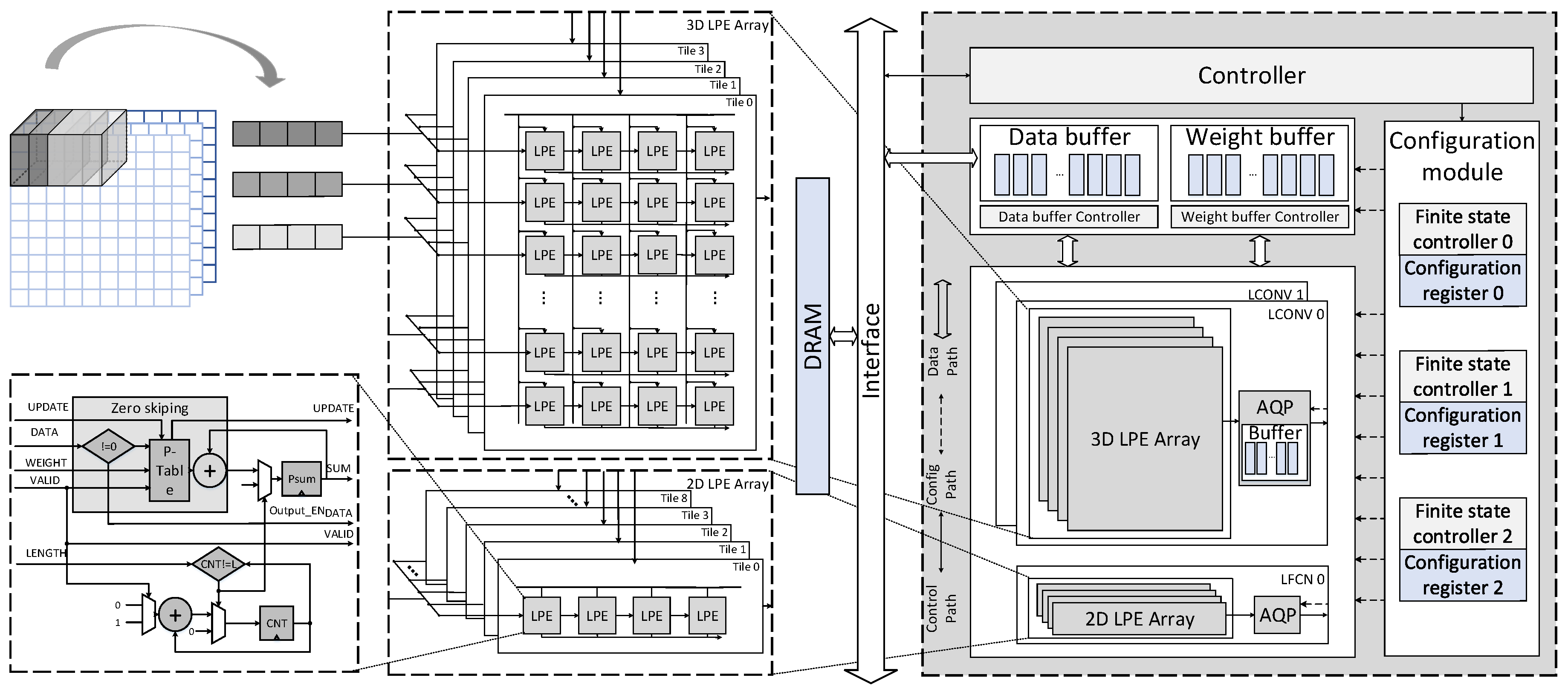
3.1. Top Architecture
Figure 4 shows the overall architecture of the CNN accelerator. It is already proved that low bit-width neural network in [
11] can also achieve competitive classification accuracy compared to 32-bit precision counterpart based on amounts of experiments. Besides, the properties of low bit-width provide more exploration space in terms of low power and high efficiency. In our work, we choose 2-bit and 1-bit as the data format of activations and weights respectively.
The accelerator is mainly composed of computing units, a memory module, a controller, and a configuration module. The computing units consist of three heterogeneous parts: two low bit-width convolutional computing (LCONV) units and a low bit-width fully connected computing (LFCN) unit for processing CONV-based layer blocks and FCN-based layer blocks, respectively. Each unit contains different subelements. For example, the LCONV unit is composed of a 3D systolic-like low bit-width processing element (LPE) array, and 16 activation, quantization and optional pooling (AQP) units. Compared to LCONV units, an LFCN unit is composed of a 2D systolic-like LPE array and an AQP unit. The dimension of computing array in CONV unit and LFC unit is 2 × 13 × 4 × 4 LPEs and 9 × 4 LPEs respectively, and the total number is 452 LPEs. The memory module includes a single port SRAM and an SRAM controller, which are both separated into the weight part and the input feature data part.
The overall execution is managed by the controller. The instructions, which can be categorized to execution and configuration, are fetched in the external memory via Advanced Extensive Interface (AXI) bus and decoded in the controller. The execution commands are responsible to initiate the execution. The configuration contexts, such as stride, number of channels, initial address and so on, are transferred to the configuration module. After receiving the configuration contexts, the configuration module reconfigures the data path, and the buffers supply data and parameters to computing units. These computing units are respectively controlled by separated configuration contexts and finite state controllers in the configuration module.
This parallel streaming architecture is very suitable for CNNs.
- (1)
CNNs have cascaded layers, which can be executed as sequential modules.
- (2)
multiple loops of intensive computation within a layer can be partitioned and executed in parallel conveniently.
- (3)
the CNN accelerator should handle large batches of classification tasks based on the application requirements.
3.2. 3D Systolic-Like Array and Dataflow
3.2.1. Merging Bit-Wise Convolution and Batch Normalization into One Step
We combine the bit-wise convolution operation with the batch normalization, on account of their common linear characteristics. In this way, we can operate the CONV layers and batch normalization layers together without any latency, additional consumption or silicon area overhead.
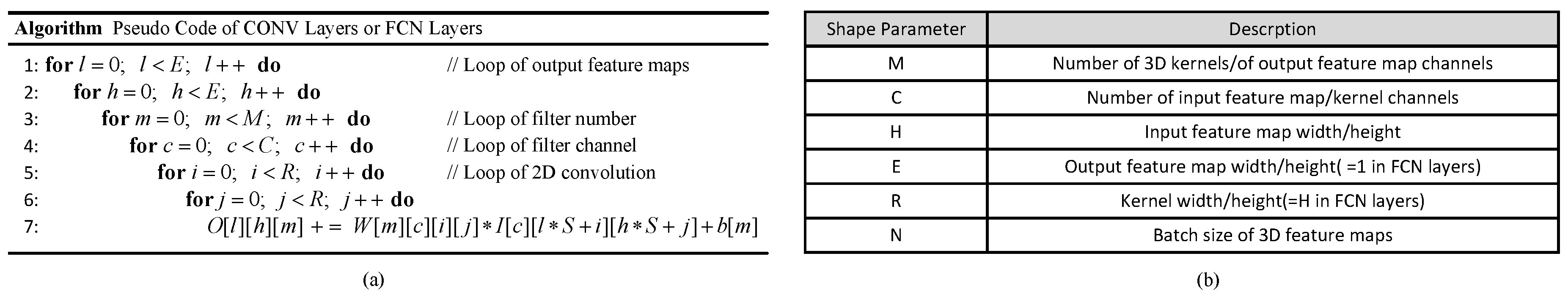
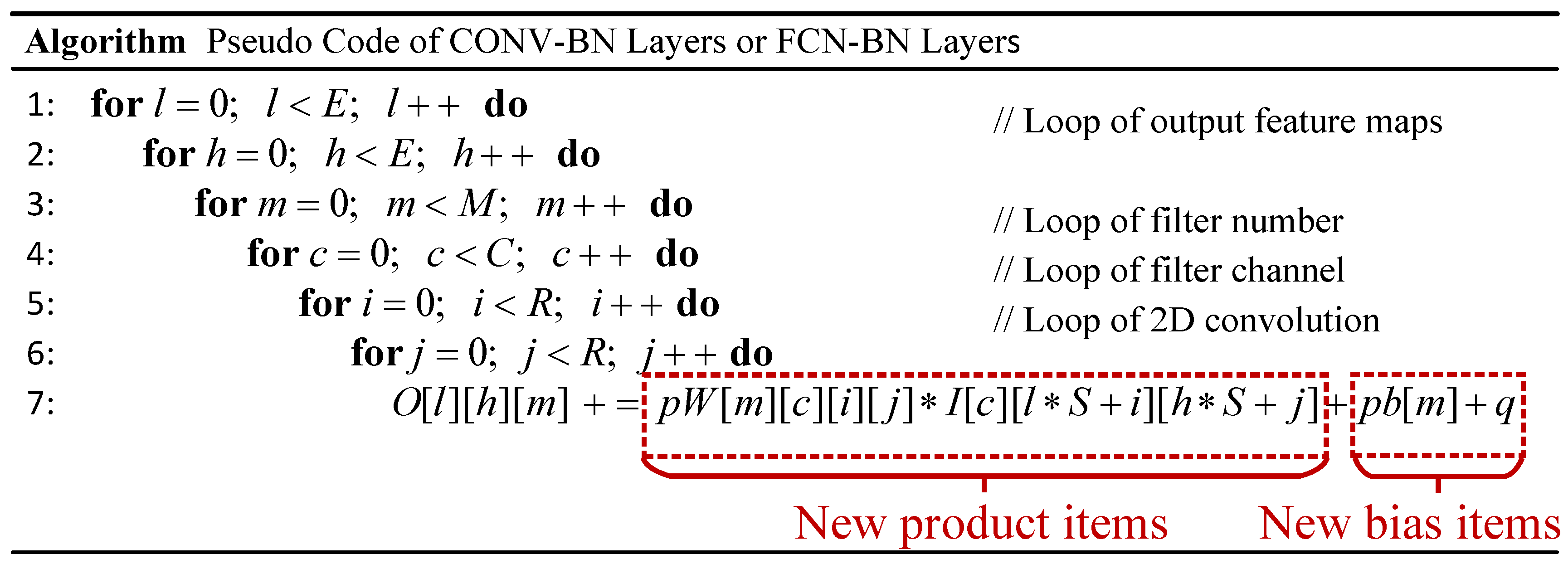
The computation expression of the convolution is demonstrated in
Figure 1. The batch normalization stacked behind will transform the expression linearly by factors of
,
,
and
, which can be formulated as (
4). We merge the similar terms, thus
where
p equals to
,
q equals to
, and these two parameters can be pre-computed offline.
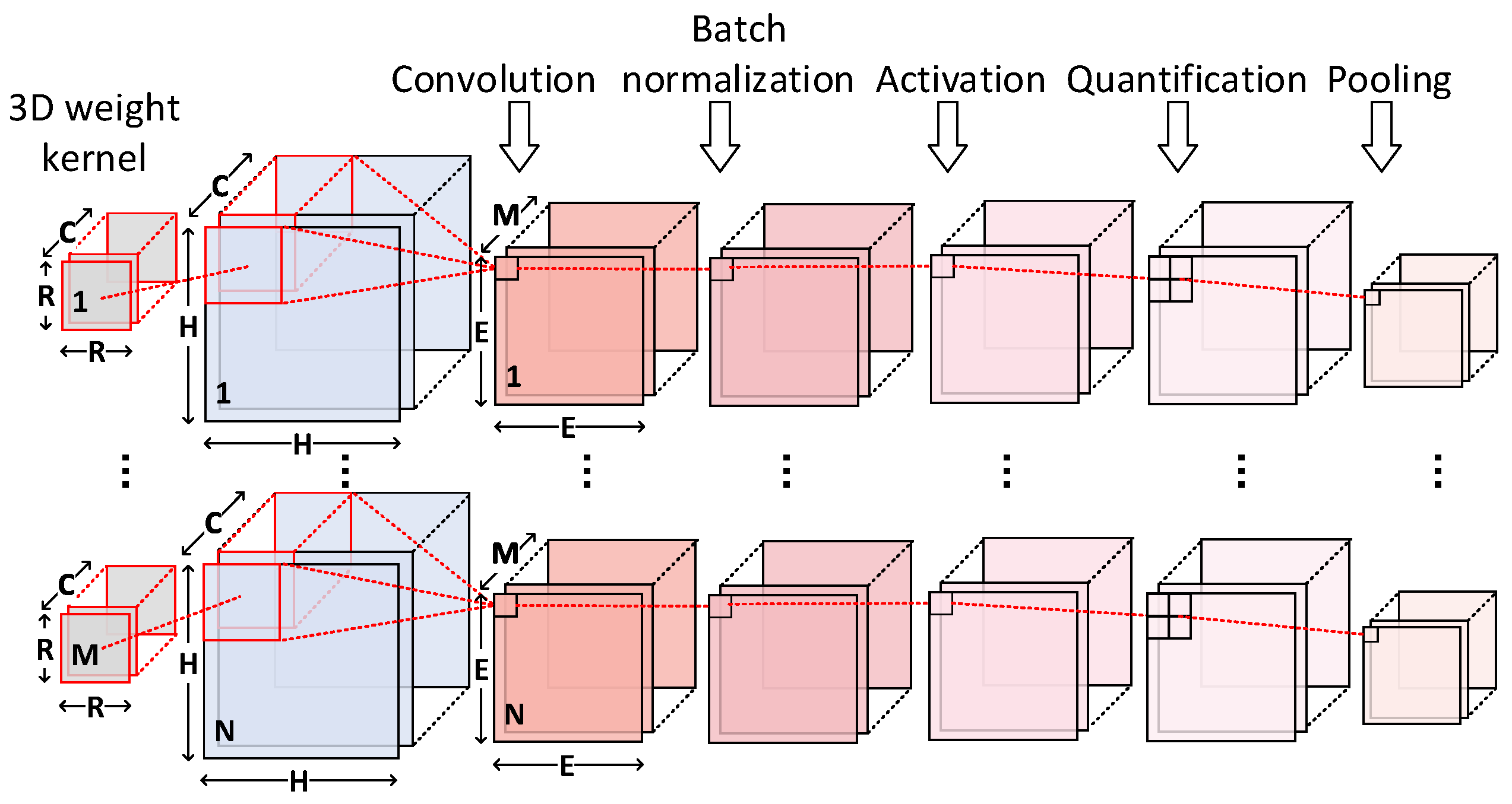
As shown in
Figure 5, the results of the combination of CONV or FCN layers and batch normalization layers can be obtained by multiplying each product item with
p and adding
q to each bias item.
3.2.2. 3D Systolic-Like Array
In the original bit-wise convolution, the product of 1-bit weight and 2-bit activation has eight possible values. According to the optimized combination, we only need to change the pre-computed values stored in the local buffer and modify the bias values before parameters are sent to the weight buffers from the external memory. These additional operations will be finished offline, and operate without any overhead in hardware. Systolic arrays can date back to 1980s. However, history-aware architects could have a competitive edge [
31]. In this work, we adopt the systolic array as our basic computing architecture. By the systolic dataflow, data can be continuously streamed along two dimensions of an array and processed in a pipelined fashion. When accelerating the CONV layers, we further improve data reuse by extending a conventional 2D array to a 3D tiled array for the intensive computation.
Figure 4 shows that a fixed number of rows are clustered to form a tile. Each tile has three groups of IO ports at the left, upper and bottom edges. The input feature data are loaded at the left edge and are horizontally shifted to the LPEs inside the tile on every cycle, weights are broadcasted to LPEs located in the same column. The outputs are locally generated on each LPE, and they are shifted to the edge of the array in the same direction with the input feature data. This dataflow is known as the output stationary defined in [
19].
As shown in
Figure 4, we introduce an LPE unit as the basic processing element, which executes local multiply accumulations. Besides, it also supports zero-skipping. An LPE unit mainly consists of a product table and an adder. The table can be updated by the same approach of transferring data in the array. The LPE can process one pair of the input feature data and weight at one cycle. In these trained models, the possibility that zeros occur among the values of activations is generally more than 30%. As known to all, multiplications with operand zero are ineffectual, besides, the zero products have no impact on the partial sum. In our design, multiplications with zero operands have been eliminated to reduce the power consumption.
3.2.3. Multi-Pattern Dataflow
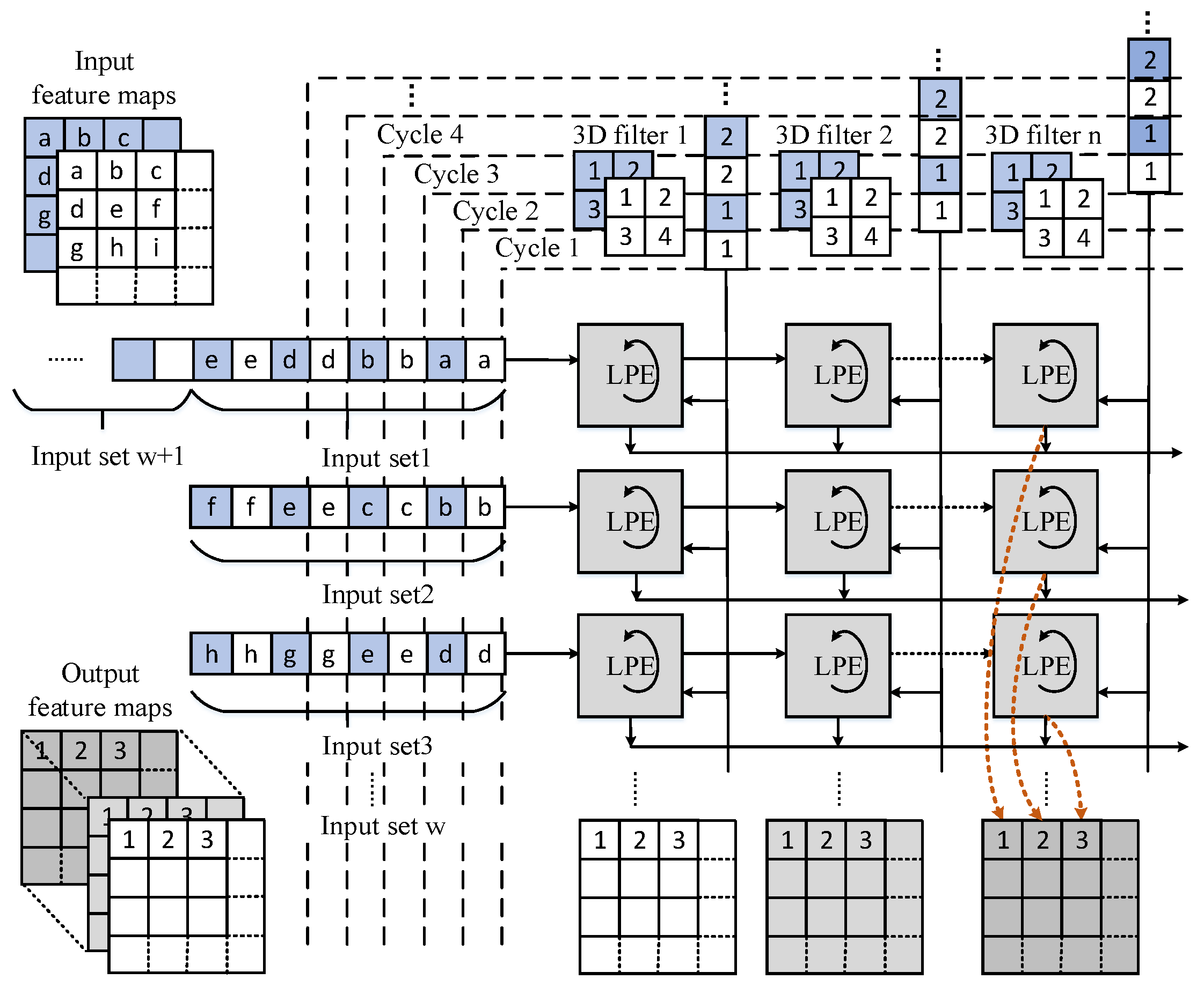
From an overall perspective, the input feature data are processed by three computing units one by one. In the LCONV units, the computing begins with feeding the input feature data and weights to the first 3D tiled systolic array LCONV0 for convolutional operations by the output stationary dataflow. In this way, inside a tile, as shown in
Figure 6, the LPEs of the same column will generate output points located at one output feature map, whereas the output points computed in the LPEs of different columns are located at different output feature maps.
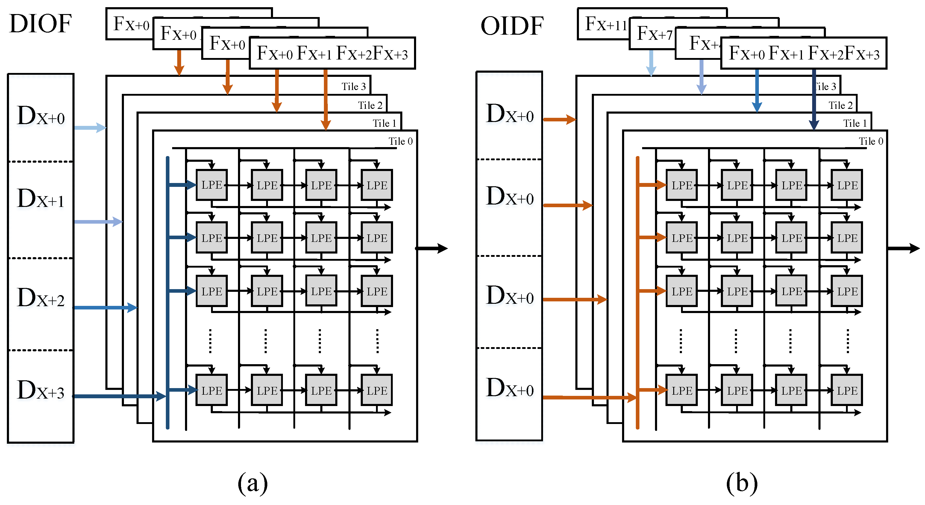
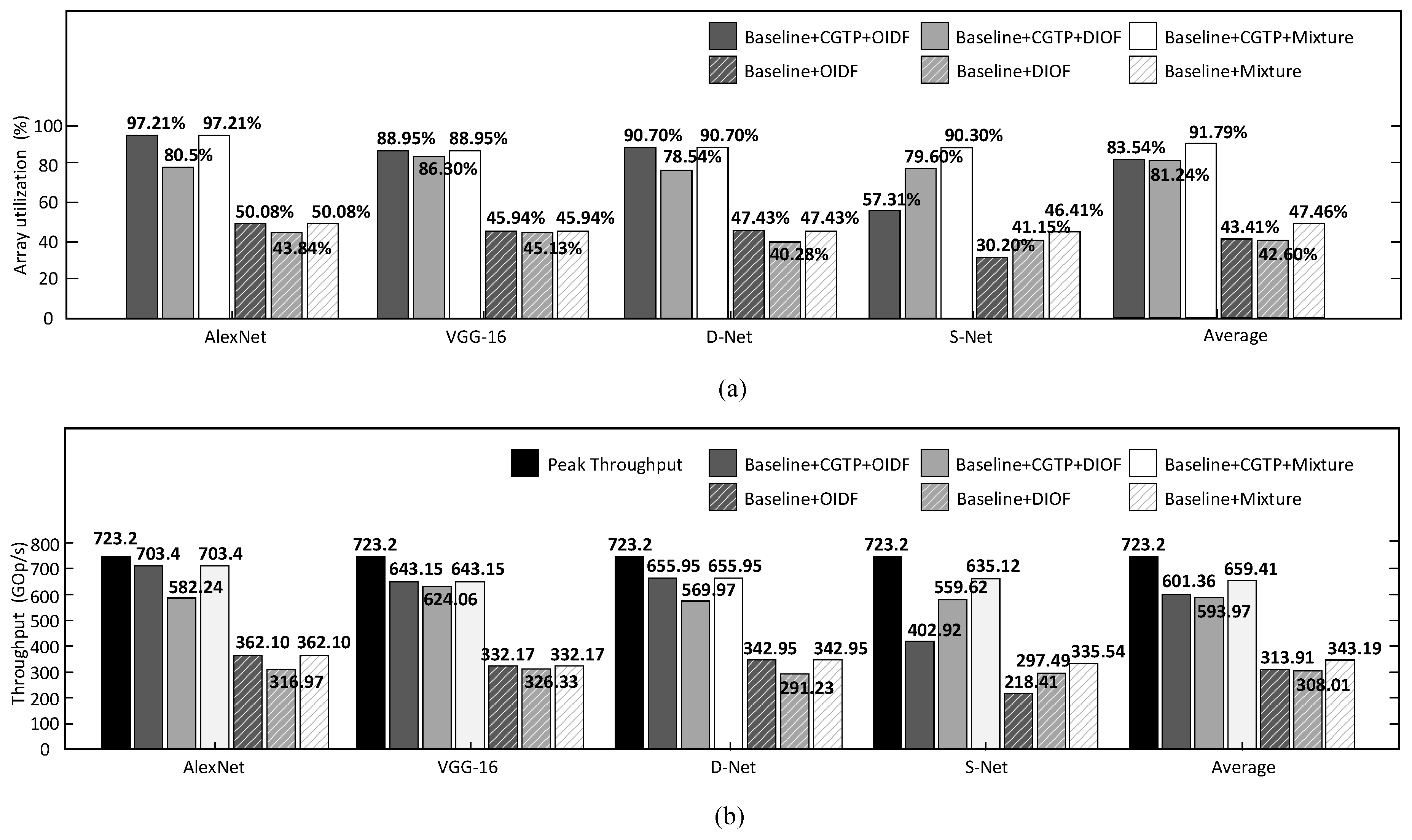
Each tile computes independently, but we can decide on the manner in which the data and weights are sent to the different tiles of the computing unit, depending on the configuration contexts, in order to improve the array use of the different sizes of CNNs. As depicted in
Figure 7, one way is that tiles share one set of input feature maps but with different sets of filters (OIDF), another is that tiles load different input feature maps only with one set of filters (DIOF). If the number of filters is much larger than
, we consider that the former dataflow is better. However, if the number of the filters is much less than
, the second way should be selected to cater to the less-filters CONV layers.
This architecture is flexible to be used with any size of images and also any size of convolution kernel (e.g., , , , …), because of the dataflow inside a tile which gives the priority to data along the channel in the input feature maps. However, the stride does have a limitation, which cannot be over 4, due to the bandwidth limitation of SRAM.
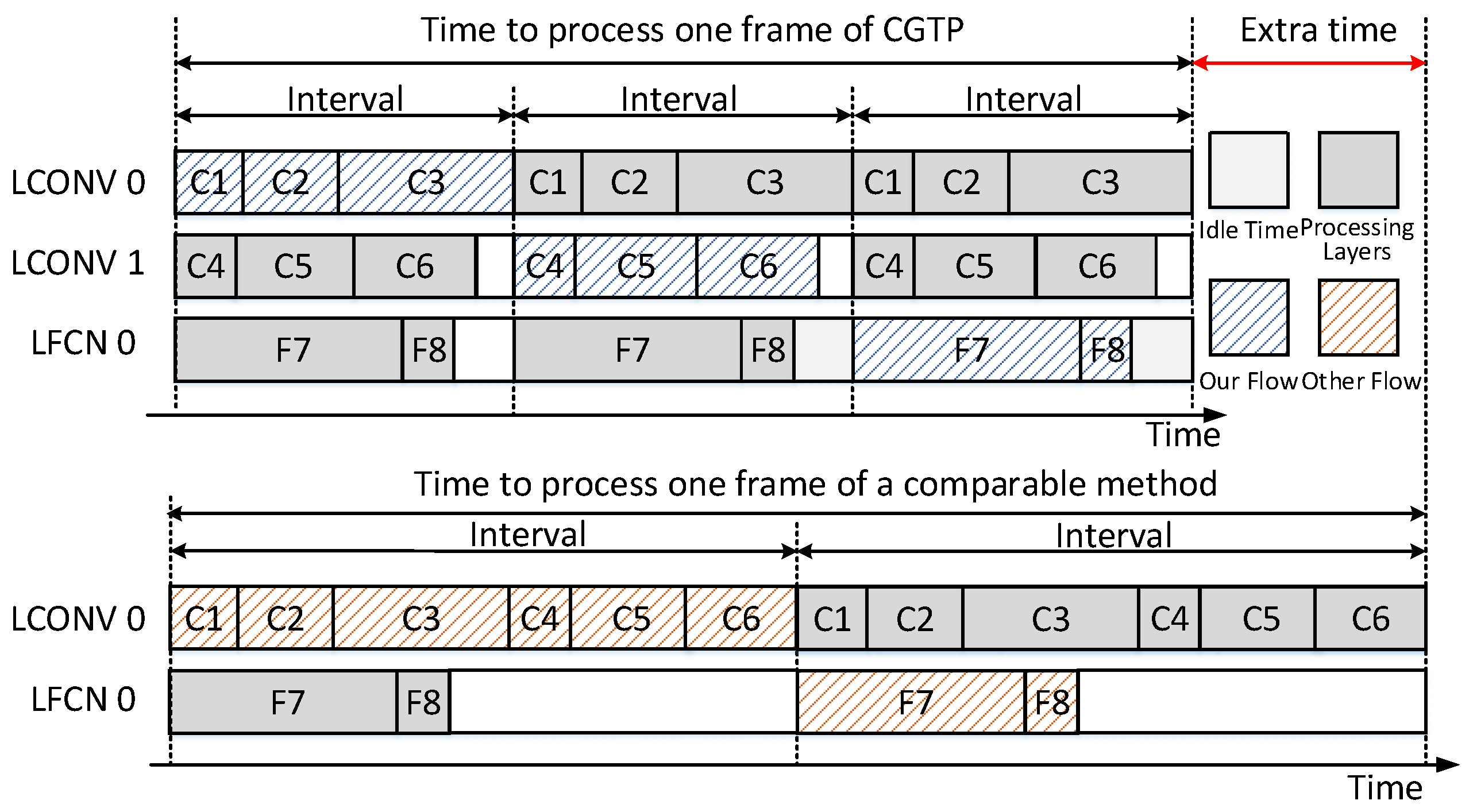
3.3. Coarse Grain Task Partitioning Strategy
Tasks can be partitioned and allocated to several computing units in coarse or fine granularity. The coarse grain indicates that the partition works on the inter-layer level, while fine grain refers to partition works on the intra-layer level. Compared to the fine granularity, the coarse granularity partitioning can reduce the communication overheads between computing units, and avoid much control and configuration logic. Our design regards one layer processing as the minimum task, which cannot be further divided.
If tasks are not well partitioned, they will introduce the large load imbalance. The computing units holding easy tasks will be compelled to wait for the units bearing heavy tasks. Thus, the slowest computing unit will dominate the throughput. To address this problem, the coarse grain task partitioning (CGTP) strategy is proposed to keep the loads of two LCONV units as balanced as possible. The CONV and FCN layers contribute to almost all the computations and storage of CNNs, whereas other layers can be omitted. The FCN layers can be regarded as CONV layers when the size of input feature maps and filters are the same. Due to the limited hardware resources, it is necessary to unroll the loops and parallelize the low bit-width CNNs onto our existing hardware with a certain number of iterations [
32]. Suppose the size of computing array is
. Accordingly, the parallelism should be
. The computing cycles of a single CONV layer is divided into two kinds, one is the OIDF dataflow case:
and another is the DIOF dataflow case:
In addition, as for FCN layers, the computing cycles can be calculated by the following formula:
In our design, the layers of a CNN model are separated into three groups, which correspond to three tasks. Each group of layers will be mapped into one computing unit. In this work, we allocate an independent computing unit LFCN0 for FCN layers due to its low parallelism. Thus the problem is simplified into dividing CONV layers into two groups. Hence, we design Algorithm 1 to obtain two groups with the roughly equal runtime. Firstly, we get the whole processing time of a CNN model from the first loop computing. Secondly, during each pass in the second loop, it adds the processing time of each CONV layer one by one iteratively, and store the current and the last accumulated time. Then a series of comparisons will be made among these values to decide which group the current CONV layer should join.
| Algorithm 1 Coarse Grain Task Partitioning |
Input: Number of CONV layers L; detailed dimensions of each CONV layer ; detailed dimensions of LCONV ; dataflow mode
Output: Two groups - 1:
fordo - 2:
if Dataflow is OIDF then - 3:
- 4:
else - 5:
- 6:
end if - 7:
- 8:
end for - 9:
fordo - 10:
if Dataflow is OIDF then - 11:
- 12:
else - 13:
- 14:
end if - 15:
- 16:
if then - 17:
add l to - 18:
else - 19:
if then - 20:
add l to - 21:
else - 22:
add l to - 23:
end if - 24:
end if - 25:
end for - 26:
Return
|
3.4. Reconfigurable Three-Stage AQP Unit
3.4.1. Modified Quantification
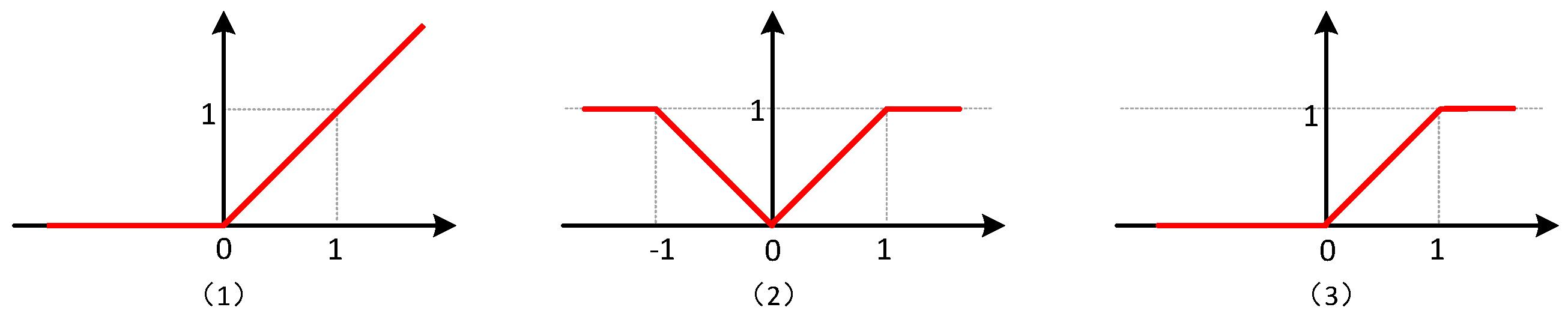
The layers of activation, quantification, and optional pooling can also be adjusted by some transformations to simplify the executing process. For example, Equation (6) shows that the outputs from CONV or FCN layers will be activated by taking the minimum between the absolute value of the inputs and 1, which can restrict the value to [0,1] to meet the requirement of the input range for the quantification step. As for the quantification, it is demonstrated in (
8) that the outputs will be quantized to four possible values
under the case of 2-bit quantification (
). It can be implemented by a series of comparisons between the outputs of activation layers and the thresholds of
. For example, a certain output neuron equals to
, which is bigger than
whereas smaller than
, therefore, it will be quantized to
. We make some adjustment to the original quantification function (
8). The modified function is shown below, which mainly changes the function
:
where
x represents the absolute value of the output point from CONV or FCN layers.
The modified quantification function will no longer be limited by the input range obtained by the activation, because this modified version has already taken those inputs out of the range
into account. It can achieve the same effect with the previous activation and quantification functions. Besides, this modified quantification function also applies for the second activation function (
7) where
x denotes the output point from CONV or FCN layers.
3.4.2. Architecture of AQP Unit and Dataflow
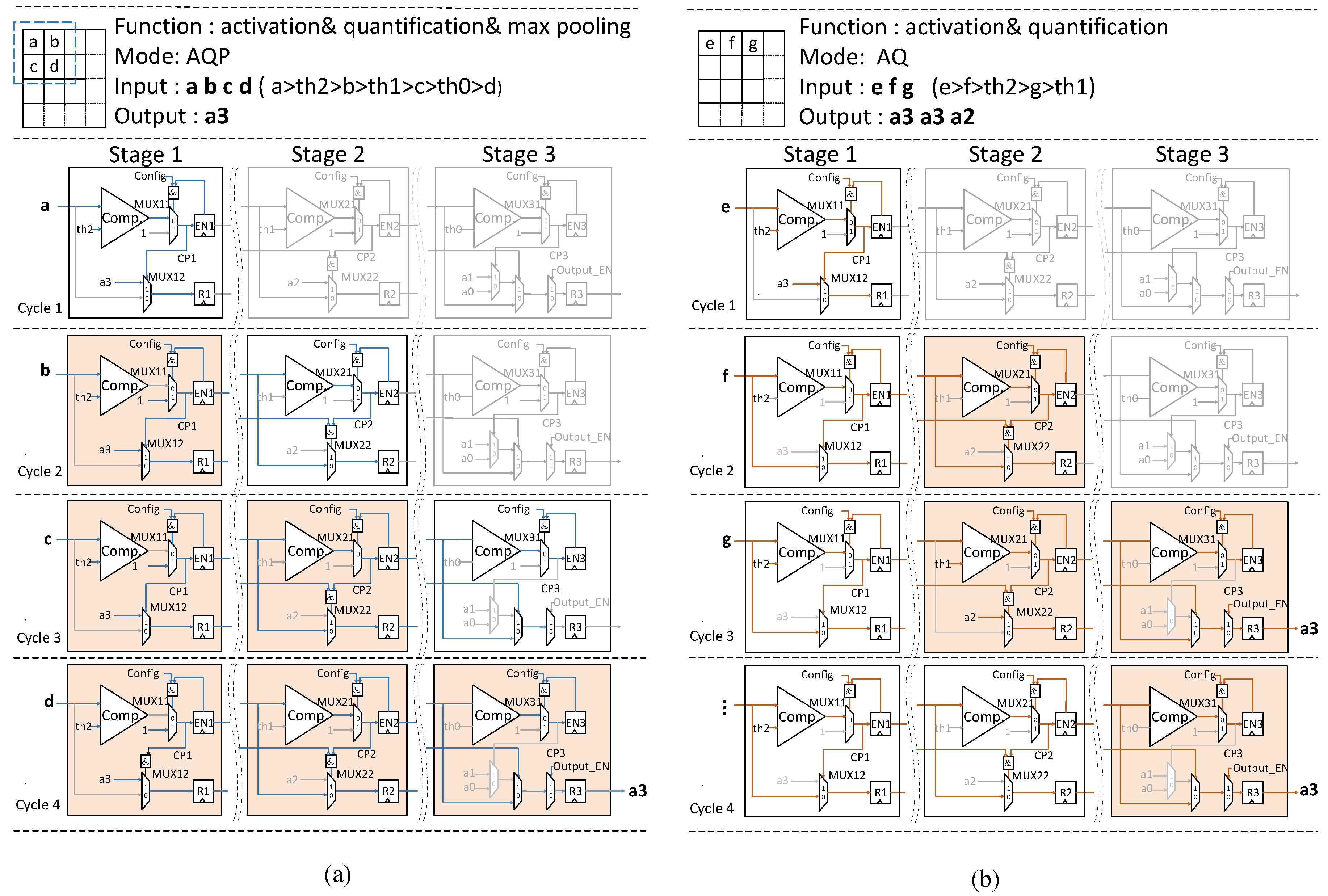
The MaxP layers has the similar computing pattern with the modified quantification layers mentioned above. Moreover, the max-pooling operation does not always exist in every CONV-based layers block. Therefore, it is not efficient to allocate an independent piece of hardware for it. Hence, we propose an efficient reconfigurable three-stage AQP unit, which can be reconfigured to two modes: activation-quantification-pooling (AQP) mode and activation-quantification (AQ) mode. Thanks to the design of the AQP unit, the max-pooling operation can be incorporated in the process of the activation and quantification at the hardware level, which means that processing max-pooling operations will not bring any overhead. Besides, the design can be further optimized to be more energy-saving with the staged blocking strategy. Moreover, the three-stage pipeline structure can reduce the data path delay and support flexible window size.
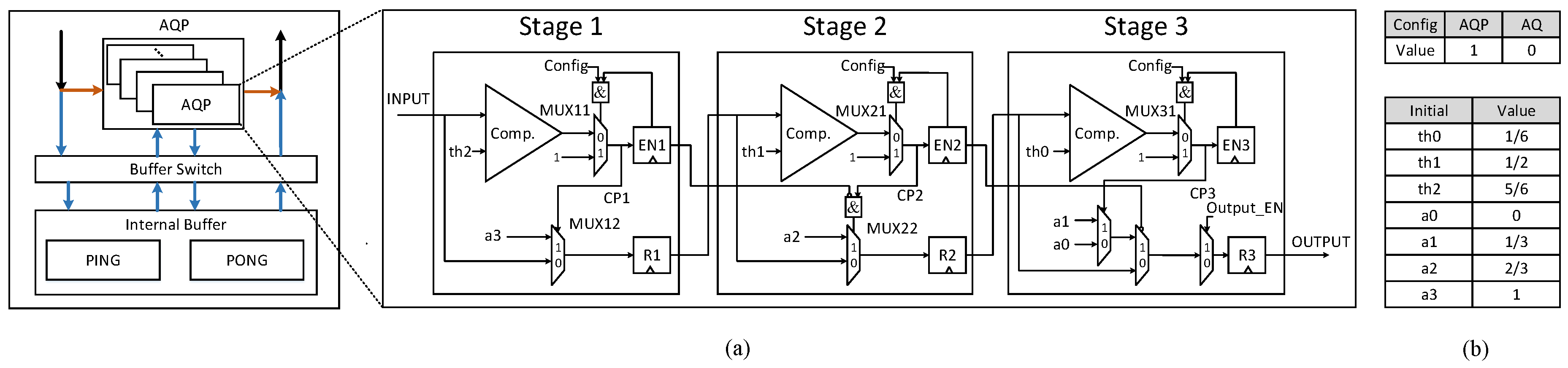
As shown in
Figure 8a, its function is controlled by a 1-bit configuration word
, which 1 denotes AQP function and 0 represents AQ function. The AQP unit is composed of three stages, each stage primarily comprises a comparator and some registers. The three-stage structure enables it to work in a pipelining way, which allows for supporting the different sizes of the max-pooling window.
As depicted in
Figure 8, the AQP module is designed as a separate part of the computing units, which mainly consists of the AQP units and the internal buffer. When
is set as AQP mode, it fetches the output feature data stored in the Ping-Pong internal buffers, which can ensure that the convolutional and AQP operation will not interfere with each other and can be processed simultaneously. Furthermore, the convolutional operation is far more computing intensive than the max-pooling operations. Therefore, the convolution can be processed in a non-stop way. When the dataflow in the 3D systolic-like array is OIDF, it will generate a portion of the data located at 16 output feature maps simultaneously over a period of continuous time. Each of 16 output feature maps has its own bank group to guarantee that data points of each output feature map can be accessed at the same time. When the dataflow in the array is DIOF, the array will produce part of data located at 4 output feature maps for a continuous period of time. In this way, every four AQP units will process data of one output feature map. When
is set as AQ mode, the data will stream into the AQP units directly without waiting in the internal buffers. There are 16 AQP units in each LCONV, and there is only one in LFC computing array.
3.4.3. Working Process of AQP Unit under Two Modes and Staged Blocking Strategy
The comparator will output positive when the operand above is bigger than the operand below.
Figure 9a shows the details of the processing in AQP mode, and the
is set as 1. For example, assumes that
are four pixels of a subregion from one feature map, the value relationship among these pixels and thresholds is:
. These four pixels enter the AQP unit one by one. At the cycle 1, the pixel
a compares with
, since
a is bigger than
, the comparison signal
turns to 1 and stored in the register
. Therefore,
is chosen as the quantification result of
a, stored in the register
in the stage 1. At the cycle 2, the pixel
b enters the stage 1 of the AQP unit, for the register
has already been set as 1 at the previous cycle, whatever the relationship of
b and
, the comparison signal
should be kept at 1 controlled by
. Therefore, the register
remains unchanged. At the same time,
in the register
passes to stage 2 and compares with
. Although
is larger than
, the signal
still remains 0 controlled by the
passed from stage 1, therefore, the output will be kept at
. In this way, the register
will keep the first comparison result
, and so on. Once the signal
turns to 1, the result stored in the register
will be sent out.
It means that if the input is bigger than the threshold at a certain stage, the register will turn to 1 to shut down the rest operations in both horizontal (the remaining pixels streaming in) and vertical (the remaining stages processing the current pixel) direction within the subregion to reduce high-low or low-high transitions.
Figure 9b depicts the details of the processing in AQ mode, the configuration word
is set as 0, it means that the comparison signal
will no longer be influenced by
of the local stage at the previous cycle, but it will still be controlled by
of the previous stage at the previous cycle. It means the set of
registers will hold back the rest operations vertically. In one sense, the register
works like a gate to block the useless operations. Due to less switching, a significant reduction in power consumption can be created.
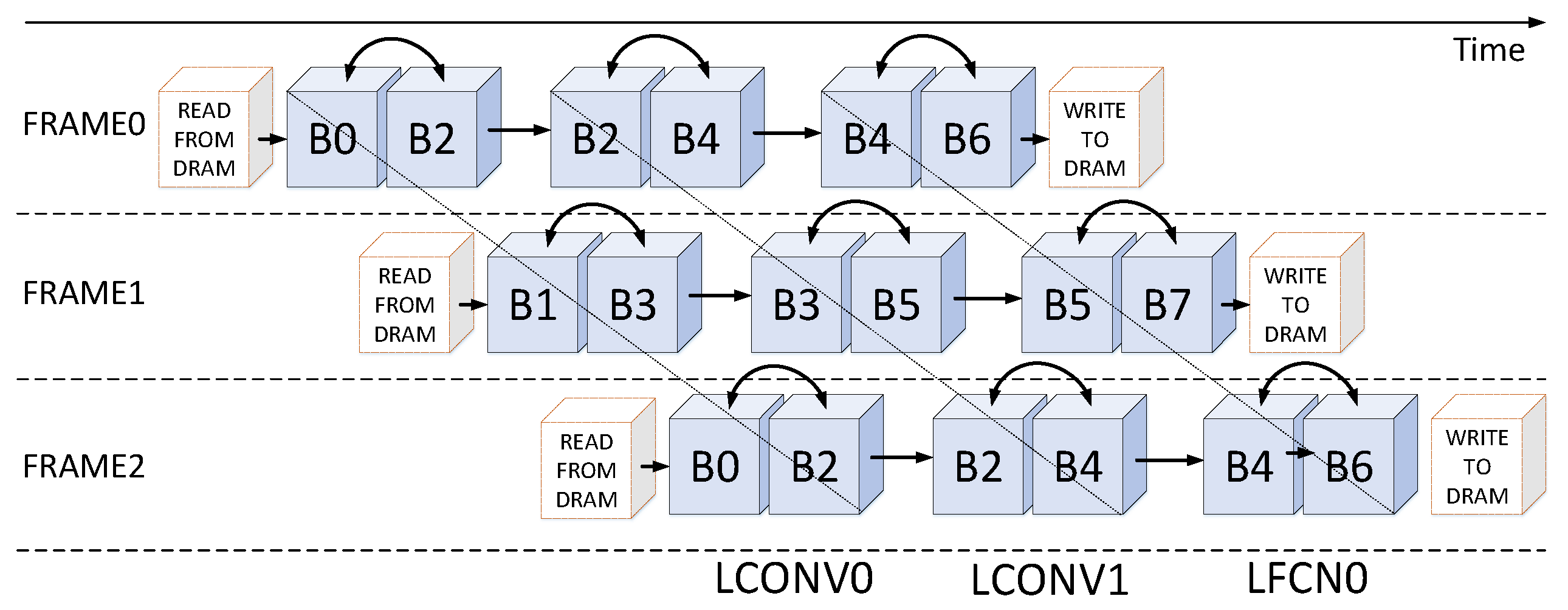
3.5. Interleaving Bank Scheduling Scheme
In order to guarantee the conflict-free data accesses and improve memory resource efficiency, an interleaving bank scheduling scheme is proposed. Algorithm 2 depicts the details.
Figure 10 shows one of the situations of the algorithm. We can observe that the multi-bank memory module can be divided at two levels:
Frame Level: the bank group 0 and the bank group 1 are loaded input feature maps of different frames from external memory alternatively. This means that all even-numbered bank groups are configured to provide and receive data on one frame, and all odd-numbered bank groups support another frame.
Computing Unit Level: each computing unit corresponds to a specific set of bank groups, for example, the LCONV0 and the LCONV1 connect to the bank group 0–3 and the bank group 2–5, respectively, the LCFN0 links to the bank group 4–7.
| Algorithm 2 Interleaving Bank Scheduling Scheme |
- 1:
represents the layer number of each group,i and j are the group index and the layer index within this group, respectively; denotes the bank group; F is number of the frames, v indicates the frame index; - 2:
// frame level - 3:
fordo - 4:
- 5:
// computing units level - 6:
for do - 7:
for do - 8:
if then - 9:
Read data from , write data to - 10:
else - 11:
Read data from , write data to - 12:
end if - 13:
end for - 14:
if then - 15:
, - 16:
else - 17:
, - 18:
end if - 19:
end for - 20:
end for
|
If the data of input feature maps is more than capacity of SRAM, the feature maps will be divided according to its row instead of the channel. Within the bank group (e.g., B0-7), there is a Ping-Pong strategy working for transferring the intermediate outputs to the external memory when the capacity of SRAM is not enough for a certain network. So actually, there is no limitation on the input size because you can always divide the input feature maps if it is too large. For example, when processing the small network like S-Net which is derived from Dorefa-net, there is no need to cache for multiple times. Besides, the time transferring data from DRAM to SRAM can be covered by computation.
Our design has two single-port SRAM, one for the data buffer and the other for the weight buffer. The data buffer is composed of 14 banks, the weight buffer is composed of 6 banks. In the data buffer, 14 banks are partitioned into 4 groups: 4-bank, 4-bank, 4-bank, 2-bank. The first three is designed for supporting the CONV layers under the streaming architecture with Ping-Pong manner. The last one is to support the FCN layers, considering that it is the last step of CNNs processing, 2 banks are enough. In the weight buffer, 6 banks are partitioned into three 2- bank groups. Each group is used to provide weights to three computing units (two LCONV units and one LFCN unit). The capacity of the data buffer is KB. The total bandwidth of each bank group is set as 104-bit, which can support the maximum stride of 4. The weight buffer is KB, and the pooling buffer is KB, which is sufficient to store the intermediate feature data.


