Abstract
Three-dimensional (3D) deconvolution is widely used in many computer vision applications. However, most previous works have only focused on accelerating two-dimensional (2D) deconvolutional neural networks (DCNNs) on Field-Programmable Gate Arrays (FPGAs), while the acceleration of 3D DCNNs has not been well studied in depth as they have higher computational complexity and sparsity than 2D DCNNs. In this paper, we focus on the acceleration of both 2D and 3D sparse DCNNs on FPGAs by proposing efficient schemes for mapping 2D and 3D sparse DCNNs on a uniform architecture. Firstly, a pruning method is used to prune unimportant network connections and increase the sparsity of weights. After being pruned, the number of parameters of DCNNs is reduced significantly without accuracy loss. Secondly, the remaining non-zero weights are encoded in coordinate (COO) format, reducing the memory demands of parameters. Finally, to demonstrate the effectiveness of our work, we implement our accelerator design on the Xilinx VC709 evaluation platform for four real-life 2D and 3D DCNNs. After the first two steps, the storage required of DCNNs is reduced up to 3.9×. Results show that the performance of our method on the accelerator outperforms that of the our prior work by 2.5× to 3.6× in latency.
1. Introduction
Recently, deconvolution has become widely used in the fields of computer vision, such as semantic segmentation [1], generative models [2], and high-resolution imaging [3]. Because 3D images exist in most medical data used in clinical practice [4], three-dimensional (3D) deconvolution has proven to be a better method than two-dimensional (2D) deconvolution in some applications.
Although the computational patterns of 2D and 3D deconvolutions are very similar, the computational complexity and memory requirements of 3D deconvolution are much higher than in 2D deconvolution, making it challenging to design efficient accelerators for them. In addition, deconvolution must insert ‘zero’ into input images before implementing convolution operations, leading to the sparsity of input images as well as the introduction of useless operations (i.e., multiplications with zeros).
Sparsity represents the fraction of zeros in deconvolutional neural networks (DCNNs), including input activations and weights’ sparsity. Exploiting the sparsity is beneficial to reduce useless computational operations. According to our study, the sparsity of the input activations of 3D deconvolution layers is higher than that of 2D deconvolution layers. As shown in Figure 1, the sparsity of deconvolutional layers in an example of 3D DCNNs (i.e., 3D Generative Adversarial Network [5] (3D-GAN)) is clearly higher than for 2D DCNNs (i.e., DCGAN [2]). As for weights, the number of weights can be reduced by and for in AlexNet and VGG-16 using pruning algorithm without accuracy degradation [6]. The high degree of sparsity in weights and activations will incur abundant useless multiplication operations and contribute to the processing engine (PE) utilization and workload imbalance [7].
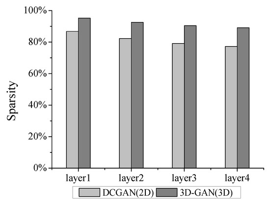
Figure 1.
Sparsity of the input feature maps in deconvolutional layers.
Many studies [8,9,10] have primarily focused on accelerating convolutional neural networks (CNNs) on Field-Programmable Gate Arrays (FPGAs), due to the beneficial high performance and energy efficiency of FPGAs. However, to the best of our knowledge, not much attention has been given to accelerate DCNNs, especially in 3D deconvolution. Given the similarities in the computational patterns of 2D and 3D deconvolutions, our previous work [11] has focused on accelerating both of them on FPGAs, using a uniform architecture. By exploiting the sparsity of input activation, our previous work can significantly avoid the number of useless multiplication operations caused by inserting ‘zero’, thereby achieving high throughput and optimum energy efficiency.
This work is mainly extended from our previous work [11]. Compared with our previous work, this work focuses on accelerating 2D and 3D sparse DCNNs on FPGA. On the basis of the uniform architecture previously proposed in [11], we further exploit the sparsity of weights and reduce the number of useless multiplication operations (that is, multiplications with zero-value weights). By pruning the low-weight connections between synapse and neurons, the weights of DCNNs are significantly compressed. Additional modules are then added into the architectures; these support the computation of sparse input activations and weights. The main contributions of this work are summarized as follows:
- A pruning algorithm [12] is creatively applied on DCNNs to remove low-weight connections and the remaining non-zero weights are encoded in coordinate (COO) format, which can significantly reduce the size of DCNNs.
- We propose an efficient mapping scheme of 2D and 3D sparse DCNNs on the uniform architecture, which can efficiently improve the parallel computational ability and computational efficiency of the accelerator.
- As a case study, we implement our design on an Xilinx VC709 board for four state-of-the-art 2D and 3D DCNNs: DCGAN, GP-GAN [13], V-Net [4] and 3D-GAN. Experimental results show that our implementation achieves an improvement of up to in performance relative to our prior work.
2. Related Work
Due to the high-performance, reconfigurability and energy-efficient nature of FPGAs, many FPGA-based accelerators [14,15,16,17,18] have been proposed that can implement CNNs; these have achieved high throughput and improved energy efficiency. Several novel reconfiguration architectures were proposed in [14] that improve the sum-of-products operations used in the convolutional kernels of CNNs. In [15], a modified Caffe CNN framework is presented; this framework implements CNNs using FPGAs, allowing transparent support to be given to individual FPGA implementation of CNN layers. In 2016, CNN-MERP, a CNN processor incorporating an efficient memory hierarchy, was produced by Han et al. [16]; this processor was shown to have significantly lower bandwidth requirements. Bettoni et al. [17] proposed an FPGA implementation of CNNs in low-power embedded systems; this study addressed portability and power efficiency. In [18], a Deep Convolutional Neural Network SqueezeNet was accelerated on an Soc FPGA by exploiting low-power consumption capabilities.
However, to the best of our knowledge, there has been little research that focuses on accelerating deconvolutions [7,19,20]. In [19,20], the researchers addressed the accelerations of the deconvolution in generative adversarial networks (GANs). Yazdanbakhsh et al. [19] introduced a new architecture to alleviate the sources of inefficiency associated with the acceleration of GANs using conventional convolution accelerators by reorganizing the output computations. In [20], an end-to-end solution was devised to generate an optimized synthesizable FPGA accelerator from a high-level GAN specification, alleviating the challenges of inefficiency and resources underutilization faced by conventional convolutional accelerators. Yan et al. [7] proposed a novel mapping method called input oriented mapping (IOM, i.e., mapping each input computation task to each PE), which can efficiently overcome the inefficiency of PE computation. All the above mentioned works, however, only consider 2D DCNNs. Our previous work [11] proposed a uniform architecture to accelerate 2D and 3D DCNNs, achieving higher performance and energy efficiency, however, did not address the problem of the sparsity of weights.
3. Background
3.1. Pruning and Encoding
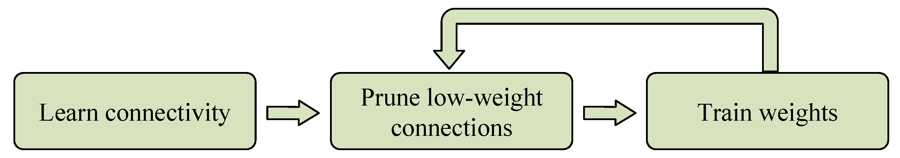
The pruning method used in this paper is proposed in [12]. The pruning method is used to reduce the number of weights which have low contribution to results, and alleviates the memory demands of the inference of DCNNs. As illustrated in Figure 2, the process of pruning consists of three steps. Firstly, the connectivity between synapse and neurons is learned by network training. Secondly, the low-weight connections are removed from the network. In this step, a threshold is defined, and those weights whose absolute values are below the threshold are viewed as low-weight connections and set to zero. Finally, the remaining sparse connections are retrained to learn the final weights. Repeat the last two steps above, until the accuracy of the network does not decline.
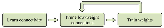
Figure 2.
Three-step pruning pipeline.
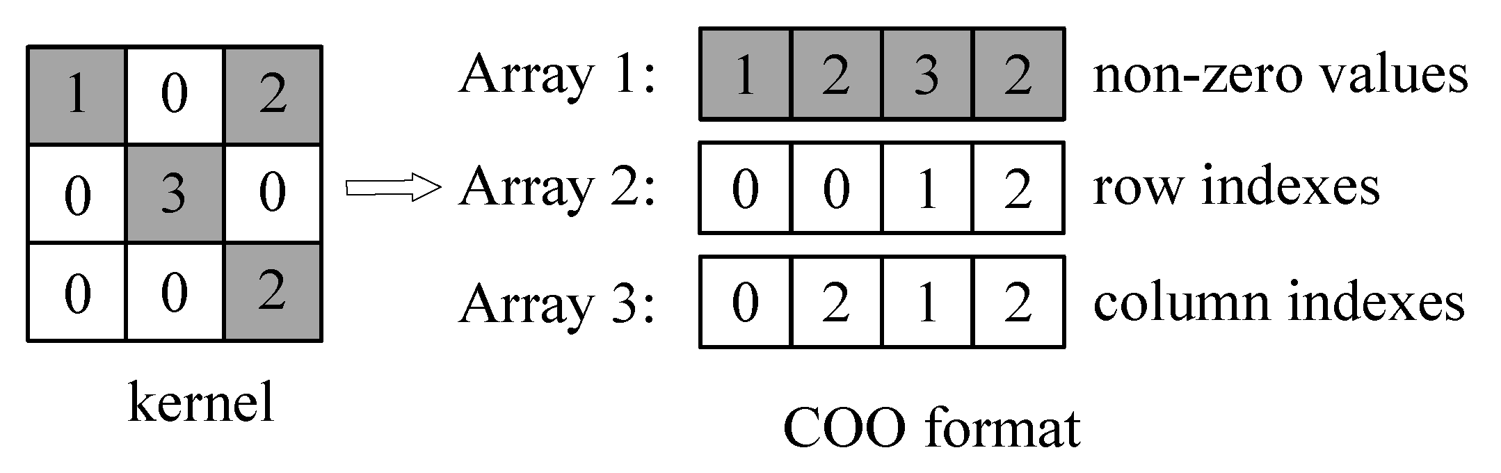
The sparse structure after pruned is stored in COO format. For a sparse matrix with n non-zero weights, using COO format to store the matrix requires numbers. As shown in Figure 3, to represent a matrix M, three one-dimensional arrays with the same length are necessary. One of the arrays stores non-zero weight values, one array stores the row indexes of non-zero weights, and the other array stores the column indexes of non-zero weights. Applying the above method can gain compressed weights. Although many other sparse matrix storage formats can be used to store sparse matrices, including compressed sparse row (CSR), compressed sparse column (CSC) and modified sparse row (MSR), the addresses of data stored in COO format can be located more quickly compared with other formats according to the indexes of data. By encoding sparse weights in COO format, the number of weights is significantly reduced.
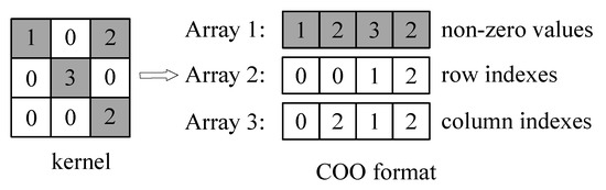
Figure 3.
Coordinate (COO) format illustration.
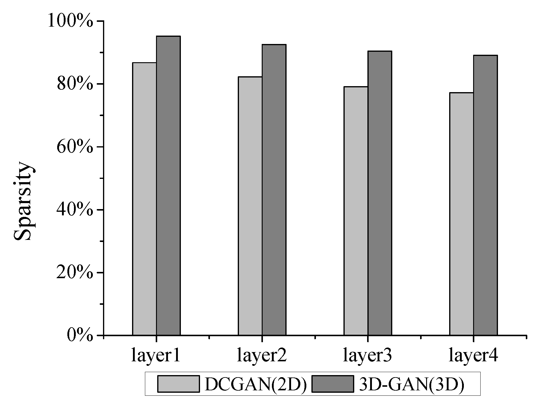
After pruning low-weight connections, the number of parameters of DCGAN and 3D-GAN is reduced to 29% and 26% of their original sizes, respectively. The detailed ratios of non-zero weights in each layer are shown in Table 1.

Table 1.
Non-zero weight ratios of DCGAN and 3D-GAN after pruned.
3.2. Deconvolution
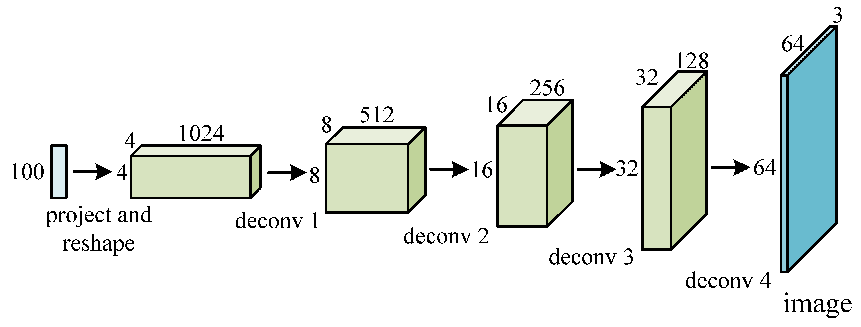
Deconvolution is the up-sampling process of increasing the size of feature maps, and the reverse process of convolution, as shown in Figure 4. The size of output feature maps of deconvolution is larger than that of input feature maps, normally twice the size of input feature maps. Deconvolution consists of two consecutive stages, including the size extension of input feature maps and the following convolution operations. The size extension requires the insertion of ‘zero’ between input activations of original input feature maps. Figure 5 shows the process of 2D and 3D deconvolutions.

Figure 4.
A real-life 2D DCNN model for image generation.

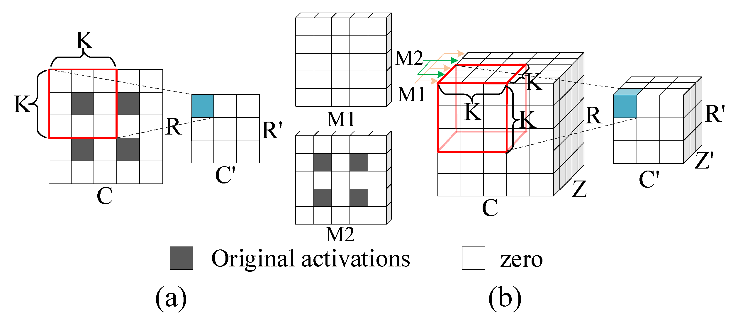
Figure 5.
Illustration of the process of deconvolutions: (a) 2D deconvolutions; (b) 3D deconvolutions.
As Figure 5a illustrates, for 2D deconvolution, the original input map is inserted with ‘zero’ shown in white between the original input activations colored in gray. A kernel then performs convolutions with the inserted feature map to generate an output map. Observed from Figure 5b, the process of 3D deconvolution is similar to that of 2D deconvolution. The original image is first inserted with ‘zero’ between the rows and columns of the 2D data tiles, which is identical to 2D deconvolution. In addition, it is also necessary to insert ‘zero’ planes (i.e., the M1 plane) between every two 2D planes (i.e., the M2 plane) and a kernel then performs convolutions with the inserted feature map to generate an output map.
4. The Proposed Architecture
4.1. Architecture Overview
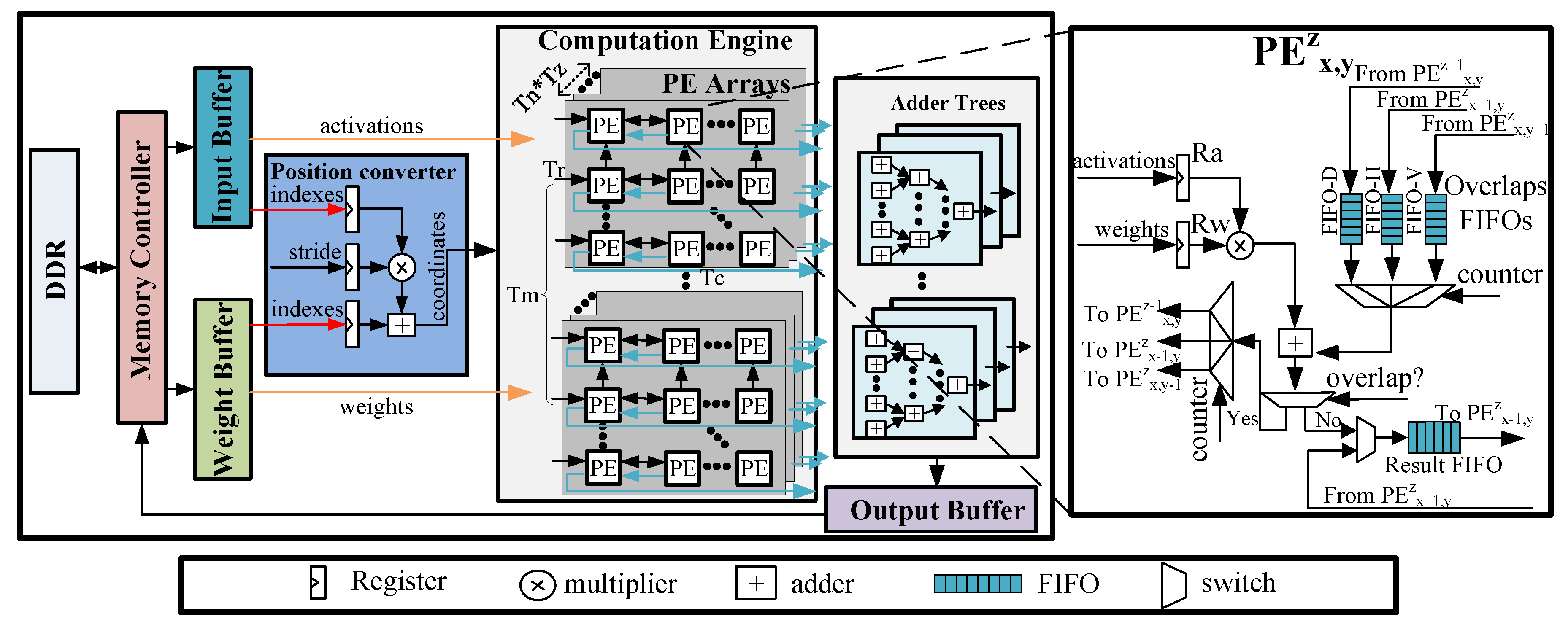
Figure 6 presents an overview of our proposed uniform architecture for accelerating both 2D and 3D sparse DCNNs. The accelerator mainly consists of a memory controller, three types of on-chip buffers, a kernel computation engine, a position converter and the adder trees. Due to a limited amount of on-chip memory of FPGAs, input images, compressed parameters and final results are stored in the off-chip memory (i.e., the dual date rate (DDR) memory). The memory controller is used to fetch the input feature maps and compressed weights from the DDR to the on-chip buffers, and storing the results into the DDR when they are available. One output feature map involves (i.e., input channels) input feature maps. However, due to the limited on-chip memory, it is difficult to cache all the input data needed for one feature map on chip. Hence, we use a blocking method to resolve this issue. Input feature maps and compressed weights are divided into some tiling blocks. We adopt three separate on-chip buffers to store tiled input feature maps, output feature maps and compressed weights.

Figure 6.
An overview of our proposed architecture.
The computation engine is a significant component of our accelerator, which consists of a group of PEs. In each group, the PEs are organized as a 3D mesh architecture, which contains 2D PE planes. In this work, we regard the PE plane as a PE array with PEs. All PEs have direct connections to the input buffers and weight buffers. Those PEs which process the input activations belonging to the same input feature maps share the same weights.
Different from our prior work [11], a position converter is added into the architecture. The position converter computes the coordinates of results yield by the computation engine according the indexes of input activations and weights. The architecture of the position converter module includes three register files, as well as an adder and a multiplier. The three register files are used to buffer input activations indexes and weights indexes, as well as to buffer sliding window stride S. The adder trees handle the additions of the results with the same positions but different input channels. adders are integrated in the adder trees to support a higher degree of parallelism.
The architecture of the PE is presented in the right part of Figure 6. It consists of two register files (i.e., Ra and Rw) to buffer the input activations and weights. In addition, three Overlap First-In-First-Outs (FIFOs) (i.e., FIFO-Vs, FIFO-Hs and FIFO-Ds) are designed to deliver the overlap of the results data from the adjacent PEs. The position converter can gain the position of results and control the data transfer between PEs. The products yielded by the multipliers are conditionally added with the data from the Overlap FIFOs. Once the current results are determined to be overlap by the position converter, they will be sent to the Overlap FIFOs of adjacent PEs, waiting to be added. Otherwise, they will be sent to the local Result FIFOs. The results in the local FIFO of the current PE will be sent to the left PE once they have stored all the local results.
4.2. Support for Sparse Weights
Several modifications to the architecture have been made to support the computation of sparse weights. Initially, sparse weights are compressed through software implementation. We store the compressed weights into weight buffers, including data and the corresponding indexes. The data relating to activations and weights (the orange lines in Figure 6) are sent to the computation engine, while their indexes (the red lines) are delivered to the position converter, which then computes the coordinates of the results.
In the position converter, the index of the input activation is multiplied by stride S; the multiplication result is then added to the weight index. When a group of adjacent input activations are fed into the computation engine, only the coordinate of the first input activation needs to be calculated. Once the coordinate of the first result is produced, other coordinates can easily be established. The coordinates of adjacent PE results just need to add stride S. The formulas are illustrated in detail in lines 9–11 of Algorithm 1 (Section 4.3). These architecture modifications will bring an increase in control logic complexity; at the same time, the consumption of hardware resources will not increase significantly.
4.3. 3D IOM Method
Previous studies [19,20] have adopted the output oriented mapping (OOM, i.e., mapping each output computation task to each PE) for the computation of deconvolution layers. This method, however, does not eliminate useless operations thereby resulting in low computational efficiency of PEs. In [7], Yan et al. proposed a novel mapping method called IOM, which can efficiently overcome the inefficiency of PE computation. Motivated by [7], we propose a 3D version of IOM for the mapping of 3D deconvolution on the accelerator.
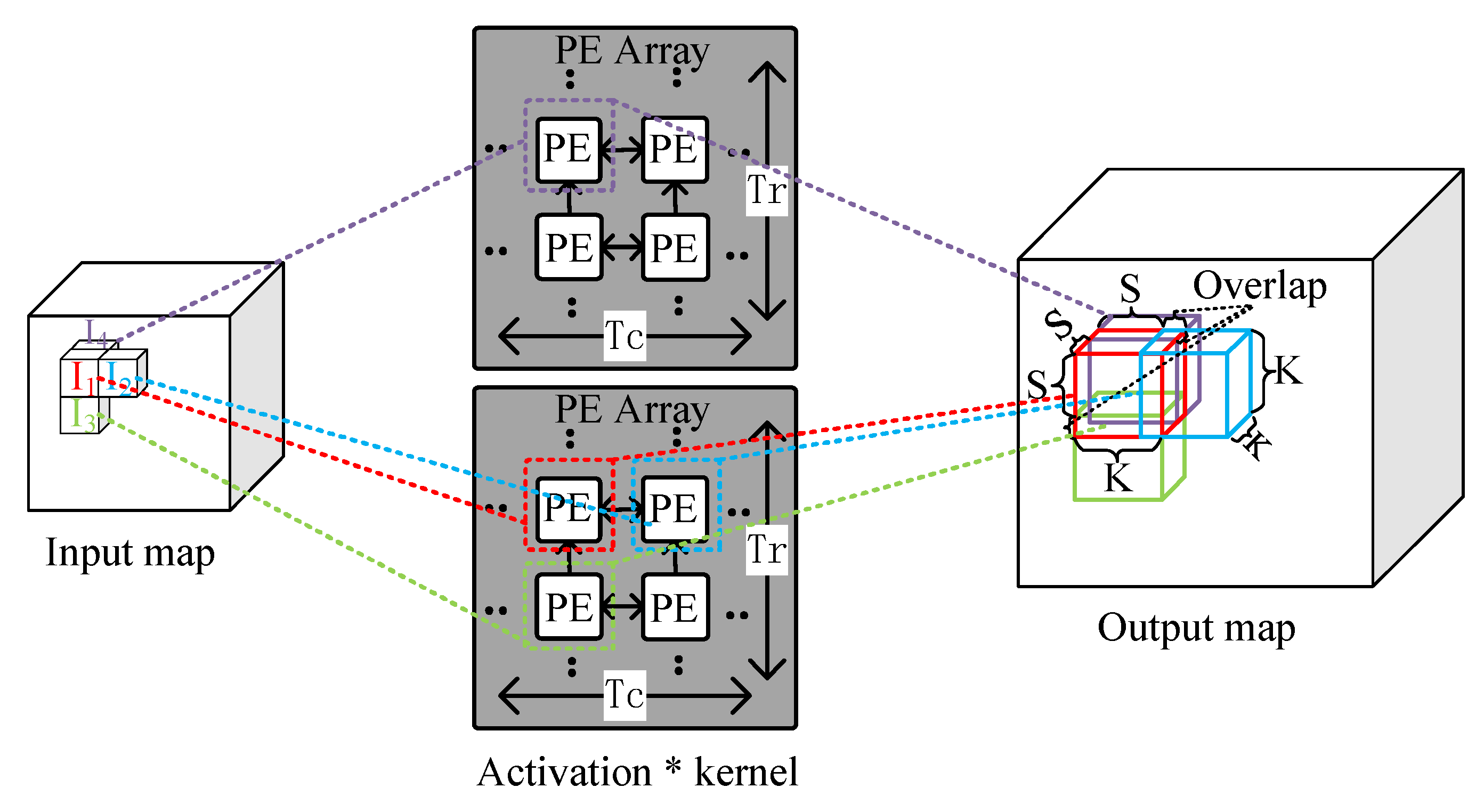
Figure 7 illustrates the 3D IOM method. ∼ are adjacent activations of the input map, and they are sent to four adjacent PEs of two PE arrays. In the PEs, each activation is multiplied by the kernel and generates a result block. The results are added to the corresponding location of the output maps. It is worth noting that some locations may overlap in the output maps and the overlapped elements of the same locations should be added up to form the resulting output maps. The overlap results from the PEs which are responsible for processing ∼ are sent to the PE which is responsible for processing , and point-wise addition is performed. In each block, the length of the overlapping part is K-S, where S is the stride.
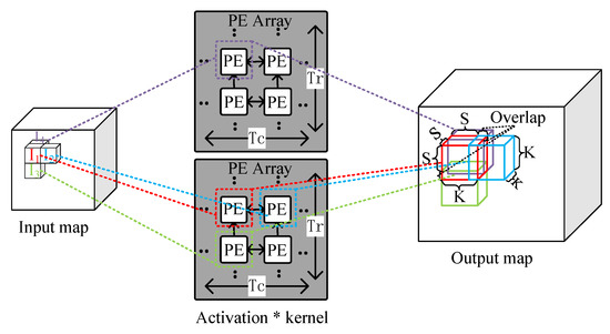
Figure 7.
Illustration of the 3D input oriented mapping (IOM) method.
In 3D deconvolution, the output feature map size is given by Equation (1). Note that represent the height, width and depth of the input maps and output maps. However, at the edge of the output feature map, there is additional data padded. Thus, the padded data are removed from the final output feature map. The final result is equal to traditional convolution with ‘zero’ inserted into the original input map. The 3D deconvolution algorithm is illustrated in Algorithm 1, where [m][][][], [n][][][] and W[m][n][][][] represent the elements of output feature maps, input feature maps and weights, respectively:
| Algorithm 1 Pseudo code for 3D deconvolution. |
|
We divide the dataflow in the PE arrays into three steps:
Loading activations and weights: Input blocks and weight blocks are firstly fetched into the input and weight buffers, and activations and weights are fed into the computation engine. Each PE in the 3D PE mesh load a input activation from input buffers, and PEs which process the input activations of the same input feature map share the same weight from weight buffers. Input activations are multiplied by all the compressed non-zero weights of the corresponding kernels. After that, the arithmetic operations of the current weights and input activations are completed in PEs, the next weights of current convolutional kernels are then fed into the computation engine. In addition, when the the arithmetic operations of the current input activations and convolutional kernels are finished, the next group activations are fed into the computation engine.
Computing: After input activations and weights are fed into the PEs, they are immediately sent to the multiplier to yield products in each PE. The results are then sent to the FIFOs. If the results overlap, they are sent to Overlap FIFOs, else they are sent to Result FIFOs. When the PEs process the overlapped part of the result blocks, the PEs load the overlapped elements from their Overlap FIFOs, and perform multiplication and additions. For 3D deconvolution, each input activation produces a result block. In result blocks, except for those results yielded by PEs, the remaining part of result blocks are regarded as zero. When the computation process in the direction of input channels (i.e., ) is completed, the position converter computes the positions of results yield by the computation engine according to the index of input activations and weights; then, results with the same locations are accumulated by the adder trees.
Writing Back: When all the activations of input blocks are completed and the overlap is accumulated, the final results (i.e., the output feature map) is transferred to output buffers. The results are accumulated until the input channels are completed, and the final outputs of output feature maps are then transferred to the external memory.
To explain this concept in more detail, we illustrate the dataflow of applying the 3D IOM method on the architecture in Figure 8. For the sake of simplicity, Figure 8 only shows the dataflow in a PE array, and the dataflow in other PE arrays is analogous. Table 2 lists the definitions used in the explanation of the dataflow.
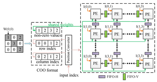
Figure 8.
Dataflow of the computation engine.
Table 2.
Definition of the parameters.
Initially, a pruned kernel is encoded in COO format. Weights are singly fed into the PE array in sequence and are shared by all PEs of the array, assuming that the size of the PE array is . In cycle 1, the first non-zero encoded weight and the input activations ∼ are fed to the PE array; the activations are then multiplied by the weight and the computation results are arranged in the output feature map according to their coordinates. The results coordinates are then computed by the position converter, as illustrated in lines 9–11 of Algorithm 1. There will be some results that have the same coordinates, leading to overlap. These computation results are overlapped in the vertical and sent to FIFO-Vs.
In cycle 2, the second non-zero weight is loaded into the PE array, which is also shared by all PEs. The weight is multiplied by the activations ∼; the computation results are then arranged in the output feature map according to their coordinates (generated by the position converter). These results have the same coordinates as the results generated in cycle 1; they are then added to the overlap loaded from FIFO-Vs (i.e., the computation results of cycle 1). These results are overlapped in the horizontal direction and sent to FIFO-Hs.
In cycle 3, the next non-zero weight is loaded into the PE array and is shared by all PEs. The weight is multiplied by the activations ∼ and the computation results are arranged in the output feature map according to their coordinates. These computation results are not overlapped and are sent to Result FIFOs.
In cycle 4, the final non-zero weight is loaded into the PE array and is multiplied by the activations ∼. These results have the same coordinates as the results generated in cycle 2; they are then added to the overlap loaded from FIFO-Hs (i.e., the added results of cycle 2). Then, the added results of cycle 4 are sent to Result FIFOs. Finally, the computation process of these input activations is completed, the next group of activations is fed into the PE array.
4.4. Support for the Acceleration of 2D and 3D DCNNs
Our architecture is able to support the acceleration of both 2D and 3D sparse DCNNs. For 3D sparse DCNNs, PE arrays are used for the computations of an input feature map. In this way, PE arrays can accelerate the computation of input feature maps simultaneously. For 2D sparse DCNNs, we map the computations of an input feature map onto a PE array. Since the input feature maps are two-dimensional, we can use PE arrays to compute input feature maps in the meantime, while maintaining the size of the PE arrays (i.e., ). In this case, the FIFO-D in each PE is disabled since there is no dataflow between adjacent PE arrays. Note that the dataflow in the PE arrays are identical when mapping 2D and 3D sparse DCNNs on the computation engine. Since little control logic is required for supporting both 2D and 3D sparse DCNNs in each PE, we omit the architecture details in Figure 6.
5. Experimental Results
5.1. Experiment Setup
As a case study, we evaluate our design using the same four DCNN models with our prior work: DCGAN, GP-GAN, 3D-GAN and V-Net. All the deconvolutional layers of the selected DCNNs have uniform and filters.
We quantitatively compare our FPGA implementation of 2D and 3D sparse DCNNs with our prior work. We also use Xilinx VC709 to evaluate our accelerator. The VC709 platform contains a Virtex-7 690t FPGA and two 4 GB DDR3 DRAMs.
Table 3 illustrates the configuration of the parameters of our benchmarks. We use the same configuration of parameters with our prior work. Note that we use the same bit width 16-bit fixed activations and weights for all the benchmarks in our experiment. To avoid the reconfiguration overhead, we use an accelerator with fixed configurations for all the benchmarks. We use PEs in total.
Table 3.
Configurations of the computation engine.
5.2. Performance Analysis
Initially, we apply a pruning algorithm on the four neural network models, retrain these model without accuracy degradation, and gain sparse weights. As Figure 9 shows, after pruning low-importance connections between synapse and neurons in neural networks without accuracy degradation, the overall sparsity of weights can be up to 70%, and be significantly compressed in the size of parameters. By compressing the weights, the number of arithmetic operations and time of inference can also be reduced significantly.
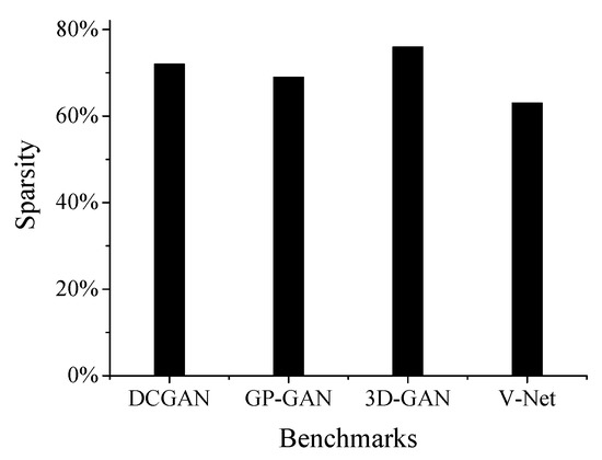
Figure 9.
Overall sparsity of weights.
Table 4 reports the resource utilization of our accelerator. The Digital Signal Processors (DSPs) and Look-up Tables (LUTs) dominate the resource consumption, and are mainly utilized for implementing multipliers and adders, respectively. Compared to our prior work, the utilization of LUTs and Flip-Flops (FFs) is increased slightly, due to the use of the position converter component.
Table 4.
Resource utilization of Xilinx VC709.
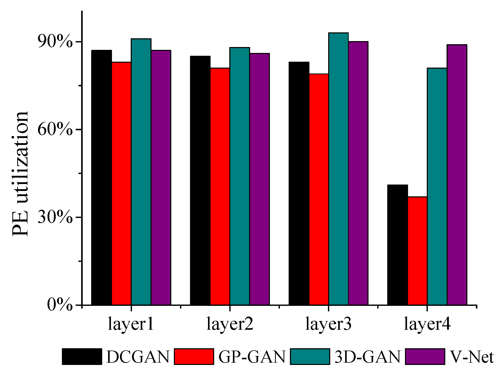
Figure 10 presents PE utilization about the accelerator. Note that the PE utilization is defined as the ratio of the computation time occupied in total time. For all benchmarks, our accelerator can achieve up over 80% of PE utilization. It demonstrates the effectiveness of our mapping and the uniform architecture for 2D and 3D deconvolutions. Note that the fourth layers of DCGAN and GP-GAN are bottlenecked by the memory access, which results in a reduction of PE utilization. Because the hardware architecture is similar to our prior work, PE utilization is quite close to it.
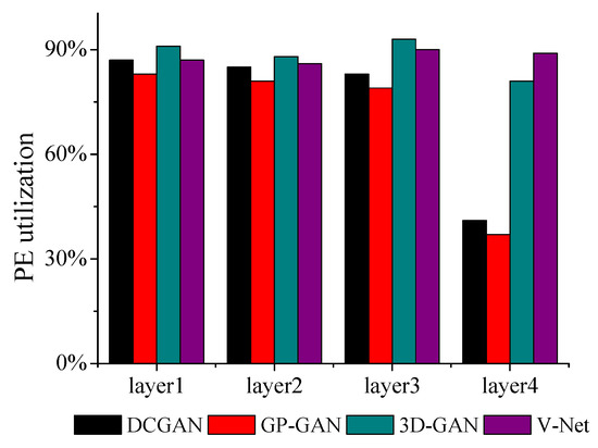
Figure 10.
Processing elements (PE) utilization.
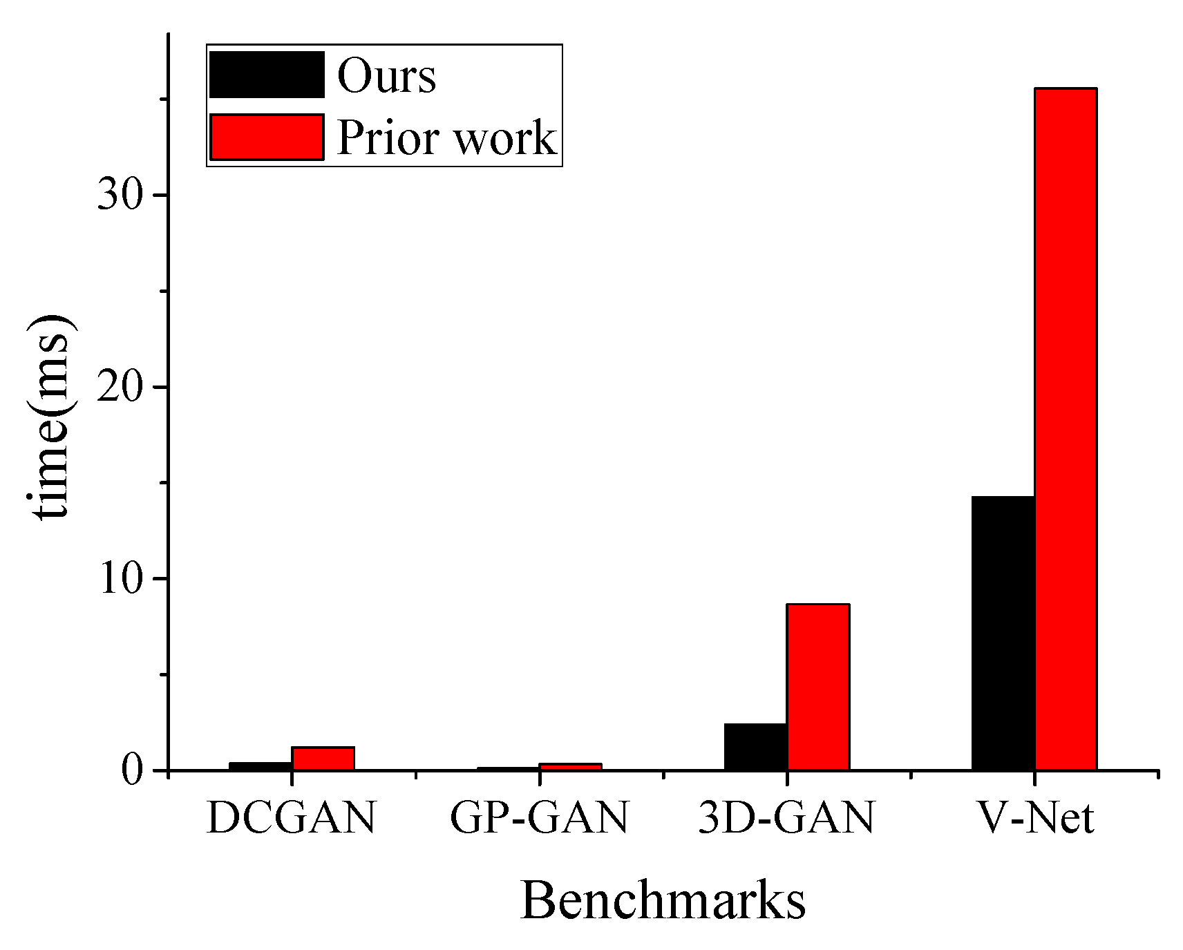
For the benchmarks in our experiment, we compare the running time of this work with that of our prior work as shown in Figure 11. The performance of our method on the accelerator outperforms that of the our prior work by to . Due to the significant sparsity of weights, our method can avoid useless arithmetic operations and then reduce the running time.
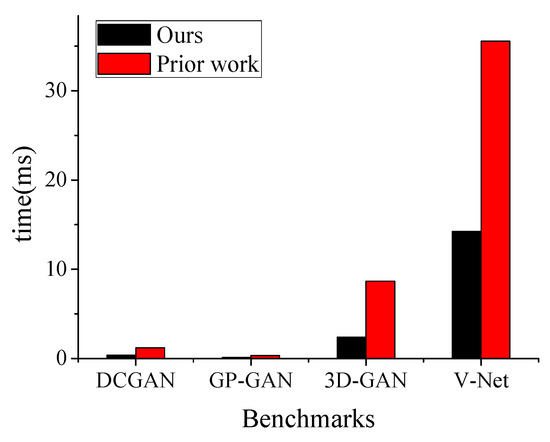
Figure 11.
Performance comparison with our prior work [11].
A comparison of our work and a previous work of 2D DCNNs is illustrated in Table 5. Because the experimental results of other works are unavailable, they are not included in the comparison. It can be seen that our work outperforms [7] in terms of throughput. However, the comparison is a bit unfair due to the different platforms and models.
Table 5.
Comparisons with previous works for 2D DCNNs.
5.3. Sensitive to Weights Sparsity
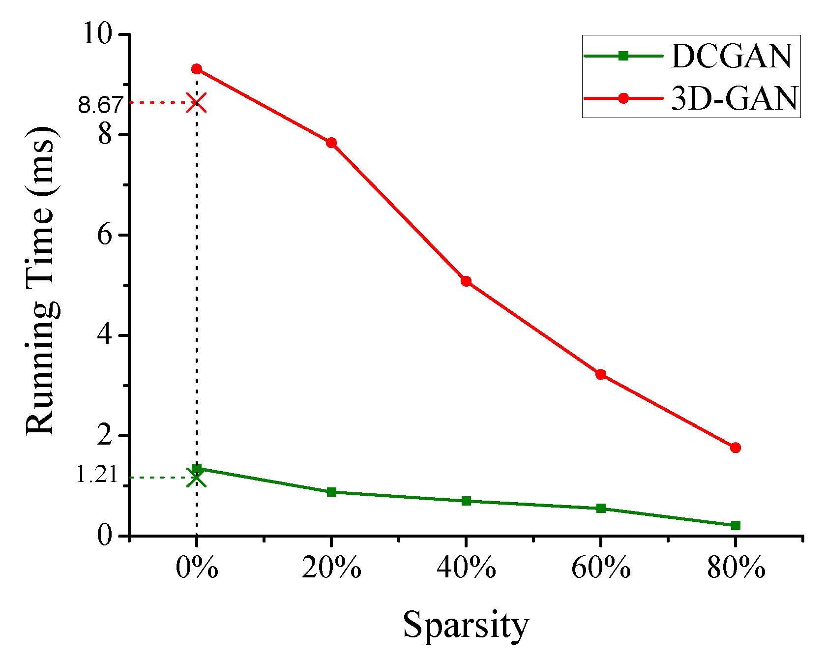
To explore the effects of weights sparsity on the performance, we examine two representative models (i.e., DCGAN and 3D-GAN) to measure the performance. In the two models, we manually set the sparsity of weights from 0 (i.e., fully dense) to 80%, ignoring the accuracy of neural networks models. Figure 12 shows that, like the growth of weights sparsity, the improvement of performance is roughly linear.
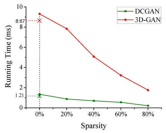
Figure 12.
Performance as a function of the sparsity of weights.
However, when the sparsity of weights is zero, the performance of this work is slightly lower than our prior work because it suffers from the cost of position transformation. From Figure 12, we can see that our method can support sparse and dense weights, and gain better performance with the increase of weights sparsity.
6. Conclusions
In this paper, we proposed a 2D and 3D deconvolution accelerator based on a uniform architecture on FPGA to support the acceleration of DCNNs with sparse weights. We employed an efficient mapping scheme of 2D and 3D deconvolutions on this architecture. By exploring the sparsity of weights, and applying data transference between adjacent PEs, our design is capable of accelerating both 2D and 3D DCNNs with sparse weights efficiently. Experimental results show that our design can achieve a great acceleration of to compared with our prior work. As future work, we plan to investigate the sparsity of feature maps of DCNNs.
Author Contributions
Conceptualization, D.W., J.S. and M.W.; methodology, D.W., J.S. and C.Z.; software, D.W., J.S. and M.W.; validation, D.W., J.S. and C.Z.; writing—original draft preparation, D.W.; writing—review and editing, D.W. and J.S.; supervision, M.W. and C.Z.
Funding
This work was supported by National Program on Key Basic Research Project 2016YFB1000401 and 2016YFB1000403.
Conflicts of Interest
The authors declare no conflict of interest.
References
- Long, J.; Shelhamer, E.; Darrell, T. Fully convolutional networks for semantic segmentation. In Proceedings of the IEEE Conference on Computer Vision and Pattern Recognition, Boston, MA, USA, 7–12 June 2015; pp. 3431–3440. [Google Scholar]
- Radford, A.; Metz, L.; Chintala, S. Unsupervised representation learning with deep convolutional generative adversarial networks. arXiv 2015, arXiv:1511.06434. [Google Scholar]
- Dong, C.; Loy, C.C.; Tang, X. Accelerating the super-resolution convolutional neural network. In Proceedings of the European Conference on Computer Vision, Amsterdam, The Netherlands, 8–16 October 2016; Springer: Berlin/Heidelberg, Germany, 2016; pp. 391–407. [Google Scholar]
- Milletari, F.; Navab, N.; Ahmadi, S.A. V-net: Fully convolutional neural networks for volumetric medical image segmentation. In Proceedings of the 2016 Fourth International Conference on 3D Vision (3DV), Stanford, CA, USA, 25–28 October 2016; pp. 565–571. [Google Scholar]
- Wu, J.; Zhang, C.; Xue, T.; Freeman, B.; Tenenbaum, J. Learning a probabilistic latent space of object shapes via 3d generative-adversarial modeling. In Advances in Neural Information Processing Systems; MIT Press: Cambridge, MA, USA, 2016; pp. 82–90. [Google Scholar]
- Han, S.; Mao, H.; Dally, W.J. Deep compression: Compressing deep neural networks with pruning, trained quantization and huffman coding. arXiv 2015, arXiv:1510.00149. [Google Scholar]
- Yan, J.; Yin, S.; Tu, F.; Liu, L.; Wei, S. GNA: Reconfigurable and Efficient Architecture for Generative Network Acceleration. IEEE Trans. Comput.-Aided Des. Integr. Circuits Syst. 2018, 37, 2519–2529. [Google Scholar] [CrossRef]
- Zhang, C.; Li, P.; Sun, G.; Guan, Y.; Xiao, B.; Cong, J. Optimizing fpga-based accelerator design for deep convolutional neural networks. In Proceedings of the 2015 ACM/SIGDA International Symposium on Field-Programmable Gate Arrays, Monterey, CA, USA, 22–24 February 2015; ACM: New York, NY, USA, 2015; pp. 161–170. [Google Scholar]
- Qiu, J.; Wang, J.; Yao, S.; Guo, K.; Li, B.; Zhou, E.; Yu, J.; Tang, T.; Xu, N.; Song, S.; et al. Going deeper with embedded fpga platform for convolutional neural network. In Proceedings of the 2016 ACM/SIGDA International Symposium on Field-Programmable Gate Arrays, Monterey, CA, USA, 21–23 February 2016; ACM: New York, NY, USA, 2016; pp. 26–35. [Google Scholar]
- Liu, Z.; Dou, Y.; Jiang, J.; Xu, J.; Li, S.; Zhou, Y.; Xu, Y. Throughput-Optimized FPGA Accelerator for Deep Convolutional Neural Networks. ACM Trans. Reconfig. Technol. Syst. TRETS 2017, 10, 17. [Google Scholar] [CrossRef]
- Wang, D.; Shen, J.; Wen, M.; Zhang, C. Towards a Uniform Architecture for the Efficient Implementation of 2D and 3D Deconvolutional Neural Networks on FPGAs. In Proceedings of the 2019 IEEE International Symposium on Circuits and Systems (ISCAS), Sapporo, Japan, 26–29 May 2019; pp. 1–5. [Google Scholar] [CrossRef]
- Han, S.; Pool, J.; Tran, J.; Dally, W. Learning both weights and connections for efficient neural network. In Advances in Neural Information Processing Systems; MIT Press: Cambridge, MA, USA, 2015; pp. 1135–1143. [Google Scholar]
- Wu, H.; Zheng, S.; Zhang, J.; Huang, K. Gp-gan: Towards realistic high-resolution image blending. arXiv 2017, arXiv:1703.07195. [Google Scholar]
- Hardieck, M.; Kumm, M.; Möller, K.; Zipf, P. Reconfigurable Convolutional Kernels for Neural Networks on FPGAs. In Proceedings of the 2019 ACM/SIGDA International Symposium on Field-Programmable Gate Arrays, Seaside, CA, USA, 24–26 February 2019; ACM: New York, NY, USA, 2019; pp. 43–52. [Google Scholar]
- DiCecco, R.; Lacey, G.; Vasiljevic, J.; Chow, P.; Taylor, G.; Areibi, S. Caffeinated FPGAs: FPGA framework for convolutional neural networks. In Proceedings of the 2016 International Conference on Field-Programmable Technology (FPT), Xi’an, China, 7–9 December 2016; pp. 265–268. [Google Scholar]
- Han, X.; Zhou, D.; Wang, S.; Kimura, S. CNN-MERP: An FPGA-based memory-efficient reconfigurable processor for forward and backward propagation of convolutional neural networks. In Proceedings of the 2016 IEEE 34th International Conference on Computer Design (ICCD), Phoenix, AZ, USA, 3–5 October 2016; pp. 320–327. [Google Scholar]
- Bettoni, M.; Urgese, G.; Kobayashi, Y.; Macii, E.; Acquaviva, A. A convolutional neural network fully implemented on fpga for embedded platforms. In Proceedings of the 2017 New Generation of CAS (NGCAS), Genova, Italy, 6–9 September 2017; pp. 49–52. [Google Scholar]
- Mousouliotis, P.G.; Panayiotou, K.L.; Tsardoulias, E.G.; Petrou, L.P.; Symeonidis, A.L. Expanding a robot’s life: Low power object recognition via FPGA-based DCNN deployment. In Proceedings of the 2018 7th International Conference on Modern Circuits and Systems Technologies (MOCAST), Thessaloniki, Greece, 7–9 May 2018; pp. 1–4. [Google Scholar]
- Yazdanbakhsh, A.; Falahati, H.; Wolfe, P.J.; Samadi, K.; Kim, N.S.; Esmaeilzadeh, H. GANAX: A Unified MIMD-SIMD Acceleration for Generative Adversarial Networks. arXiv 2018, arXiv:1806.01107. [Google Scholar]
- Yazdanbakhsh, A.; Brzozowski, M.; Khaleghi, B.; Ghodrati, S.; Samadi, K.; Kim, N.S.; Esmaeilzadeh, H. FlexiGAN: An End-to-End Solution for FPGA Acceleration of Generative Adversarial Networks. In Proceedings of the 2018 IEEE 26th Annual International Symposium on Field-Programmable Custom Computing Machines (FCCM), Boulder, CO, USA, 29 April–1 May 2018; pp. 65–72. [Google Scholar]


© 2019 by the authors. Licensee MDPI, Basel, Switzerland. This article is an open access article distributed under the terms and conditions of the Creative Commons Attribution (CC BY) license (http://creativecommons.org/licenses/by/4.0/).