Fault Tolerant Control of Electronic Throttles with Friction Changes

Abstract

To enhance the reliability of the electronic throttle and consequently the vehicles driven by the internal combustion engines, a fault tolerant control strategy is developed in this paper. The proposed method employs a full-order terminal sliding mode control in conjunction with an adaptive radial basis function network to estimate change rate of the fault. Fault tolerant control to abrupt and incipient changes in the throttle viscous friction torque coefficient and the throttle coulomb friction torque coefficient is achieved. Whilst the throttle position is driven to track the reference signal, the post-fault dynamics are guaranteed to converge to the equilibrium point in finite time, and the control is smooth without chattering. A nonlinear Simulink model of an electronic throttle is developed with real physical parameters and is used for evaluation of the developed method. A significant change of the throttle friction torque is simulated, and the fault tolerant control system keeps system stability and tracking the reference signal in the presence of the fault.

1. Introduction

Electronic throttle is an actuator to regulate the throttle plate opening to control airflow rate into the air manifold for air/fuel ratio control in automotive engines. To achieve high quality driving performance, high fuel economy, and low air pollution, an air/fuel ratio with high accuracy is required. Consequently, the airflow rate needs to be controlled accurately. Furthermore, to enhance the reliability of the vehicle operation, reliable operation of the electronic throttle against disturbance and effective control that tolerates system faults—including actuator, component, and sensor faults—are essential.

Electronic throttle is usually controlled with PID three terms control [1], auto-tuning and self-tuning adaptive control [2], and sliding mode control [3].

Many researchers have tried to detect and isolate electronic throttle faults with different methods. Conatser et al. [4] developed a linear model with nonlinear terms as disturbance for the electronic throttle. In the model, the torque due to the air flow, the torque caused by the return spring, the torque applied by the friction and the air manifold pressure, etc., are treated as disturbances. For fault detection, the nonlinear parity space method is applied with forward relation and inverse relation derived from the developed model. The system output, the throttle position, is estimated using the forward model with the measured system input, the armature voltage. The system input, the armature voltage, is estimated using the inverse model with the measured system output, the throttle position. Then, the estimation errors of the input and the output are used as the residual to detect faults. In no fault case, the residual is supposed to be a noise level due to the modeling error, while if any fault occurs, the residual deviates from noise level to reflect fault impact. Some other methods such as the unknown input observer [5] or the continuous time parameter estimation method [6] can be used. In the literature [7], a sliding mode control with sensor fault tolerance for electronic throttle was reported. A sliding mode observer is employed in the paper to estimate throttle position and compare it with sensor output for fault detection. If the difference is significant, the estimate is used instead of sensor output, thus the sensor fault is tolerant. However, the paper did not tackle the actuator and the system component faults.

Fault tolerant control is an effective strategy to enhance system reliability in fault occurrence rather than catastrophe. Recently developed fault tolerant control techniques include the use of adaptive neural networks [8], the back-stepping method [9], the terminal sliding mode control method [10], etc. For a comprehensive understanding, please see the review papers in [11,12,13,14]. Adaptive observers have been used to on-line estimate a fault, where the fault estimator can be implemented with different learning algorithms. A radial basis function (RBF) network was used in [15] and [16] as the on-line estimator, and a projection-based learning algorithm was developed. Rather than directly estimate disturbance, neural networks have also been used to estimate unknown parameters in a nonlinear uncertain system. In the air-to-fuel ratio (AFR) control of spark ignition engines using a sliding mode method [17], a radial basis function network is used to estimate two unknown parameters so that the fault can be tolerated when the estimated fault is used for compensation. Moreover, an RBF network was used to estimate the optimal sliding gain in [18] to achieve an optimal robust performance in AFR control against model uncertainty and measurement noise.

Terminal sliding mode control (TSMC) has superior features over the normal sliding mode control with fast and finite time convergence in addition to being robust against the matched disturbance and easy to implement. However, the TSMC still has two drawbacks of singularity in the design and the output chattering. Ref. [19] proposed a novel concept of full order TSMC (FOTSMC) that avoided both singularity and chattering and kept the finite time convergence. The application of the FOTSMC requires priori knowledge of the system model, specifically the bounds of derivative of system disturbance. This requirement may not be satisfied in many practical industrial applications. Therefore, this limitation needs to be eliminated to gain wide industrial applications.

In this paper, we develop a fault tolerant control system for electronic throttle based on a throttle model. In the model, the nonlinear dynamics of viscous and coulomb frictions of the motor and the throttle are considered. The discrete-time characteristics of the return spring are also considered. Throttle position tracking control with stabilization of post-fault dynamics is achieved by employing a developed FOTSMC. The fault tolerant control is achieved with guaranteed whole system stability after a fault occurs, whilst the performance of tracking is maintained in high quality by fault estimation and compensation. An RBF network is used with on-line adaptation in the framework of the FOTSMC to estimate the change rate of the fault, thus the fault compensation is enabled. A nonlinear throttle model is set up using a set of real physical parameters of the throttle. With this model, the developed control algorithm is simulated using Matlab/Simulink. Two sets of reference signals of the throttle positions of square wave and sinusoidal signals are used, and the fault is simulated with a significant change in throttle viscous and coulomb friction torque coefficients. The simulation results show that fault tolerant tracking is achieved under occurrence of the simulated friction fault; the closed-loop system maintains stability for the post-fault dynamics.

The novelty and the contributions of the work in this paper are: (a) in the developed FOTSMC, the requirement for knowing the upper bound of the considered fault change rate is relaxed; (b) the friction fault that often occurs in real electronic throttle system is tolerated, whilst the throttle position tracking control is achieved; (c) closed-loop system stability with post-fault dynamics and the convergence of the adaptive RBF network estimation are guaranteed with Lyapunov theory.

The paper is organized as follows. Section 2 presents electronic throttle modeling and fault presentation. Section 3 describes the developed fault diagnosis and the fault tolerant control method. Application of the developed method to the electronic throttles is presented in Section 4. Section 5 demonstrates the simulation results, and some conclusions are drawn in Section 6.

2. Electronic Throttle Modeling

A typical electronic throttle control (ETC) system consists of a throttle plate in the throttle body, which is driven by a direct current (DC) motor through a gearbox. The throttle plate is brought back to the close position by a returning spring mounted to the end of the throttle plate. A throttle position sensor is mounted to send back the feedback signal. A schematic of the throttle body used in the air path control of an automotive engine can be found in [4].

The rotary speed and the motor torque are transmitted to the throttle end through the gear box, where the gear ratio $=\frac{{\theta }_m}{\theta }=T_M/T_{th}$. Each part of the system is modeled to achieve the model of the total system dynamics. The dynamics of the motor rotary speed and the armature current are,

$${\dot{\theta }}_M\left(t\right)={\omega }_M\left(t\right)$$

(1)

$$L\dot{\dot{i}}\left(t\right)=V\left(t\right)-Ri\left(t\right)-K_b{\omega }_M\left(t\right)$$

(2)

The torque balance equation at the throttle end is derived,

$$\dot{\omega }=\frac{1}{N^2{J}_M+J}\left(N{T}_M-N{T}_{Mf}-T_{Tf}-T_{sp}\right)$$

(3)

where $T_{Mf}\left(t\right)$ and $T_{Tf}\left(t\right)$ are motor friction torque and throttle friction torque, respectively. $T_{sp}\left(t\right)$ is the torque due to the return spring. The other variables and parameters are listed in the nomenclature in

Table 1. Electronic throttle control (ETC) system variables and parameters.

Variable/Parameters	Definition (Units)
i	Motor armature current (A)
${\theta }_M$	Motor angular displacement (rad)
${\omega }_M$	Motor angular velocity (rad/s)
V	Motor input voltage (V)
$T_M$	Motor torque (Nm)
$T_{Mf}$	Motor friction torque (Nm)
$T_{th}$	Transmitted motor torque at throttle end (Nm)
L	Armature inductance (H)
R	Armature resistance (R)
$K_b$	Back-emf constant (V.s/rad)
$J_M$	Effective motor inertia (kg.m2)
J	Effective throttle inertia (kg.m2)
$K_r$	Motor torque constant (Nm/A)
$B_M$	Motor viscous frictional torque coefficient (Nm.s/rad)
$B_{Mf}$	Motor coulomb friction torque coefficient (Nm)
θ	Throttle plate angular displacement (rad)
ω	Throttle plate angular velocity (rad/s)
$T_{mt}$	Torque transmitted from gears (Nm)
$T_{Tf}$	Throttle frictional torque (Nm)
$T_{sp}$	Torque due to return spring (Nm)
$T_d$	Torque due to disturbance (Nm)
$B_T$	Throttle viscous frictional torque coefficient (Nm.s/rad)
$B_{Tf}$	Throttle coulomb frictional torque coefficient (Nm)
$K_{sp}$	Throttle plate return spring stiffness (Nm/rad)
$K_0$	Throttle plate return spring offsite (Nm)
N	Gear set ratio ($N={\theta }_M/\theta$)
${\mathsf{\theta }}_0$	Limp-home position (rad)

.

The friction in the motor end and the throttle end consists of two parts, one is viscous friction and the other is coulomb friction. The coulomb friction does not relate to the rotary velocity but only take its direction. Therefore, the friction torque is presented dynamically as,

$$T_{Mf}\left(t\right)=B_M{\omega }_M\left(t\right)+B_{Mf}\ast sign\left({\omega }_M\right)$$

(4)

$$T_{Tf}\left(t\right)=B_T\omega \left(t\right)+B_{Tf}\ast sign\left(\omega \right)$$

(5)

The torque due to the return spring is nonlinearly related to the throttle plate position. The spring dynamics are described as,

$$T_{sp}\left(t\right)=K_{sp}\left[\theta \left(t\right)-{\theta }_0\left(t\right)\right]+K_0\ast sign\left[\theta \left(t\right)-{\theta }_0\left(t\right)\right]$$

(6)

where ${\theta }_0$ is the default position called the Limp-Home position, at which the valve ensures the air flow just enough for the engine to keep running.

By substituting (4) to (6) into (3), we derive the following model.

$$\dot{\omega }=\frac{1}{N^2{J}_M+J}[N{K}_{r}i-(N^2{B}_M+B_T)\omega -\left(N{B}_{Mf}+B_{Tf}\right)sign\left(\omega \right)-K_{sp}\left(\theta -{\theta }_0\right)-K_0\mathrm{sign}\left(\theta -{\theta }_0\right)]$$

(7)

In the ETC system, the armature inductance is very small and therefore can be neglected. Thus, the dynamics of the armature current in Equation (3) equals zero, which leads to,

$$i\left(t\right)=\frac{1}{R}\left[V\left(t\right)-K_{b}N\omega \left(t\right)\right]$$

(8)

Substituting (8) to (7) yields,

$$\begin{gathered} \dot{\omega }=\frac{1}{N^2{J}_M+J}[\frac{N{K}_r}{R}V-(N^2{B}_M+B_T+\frac{N^2{K}_r{K}_b}{R})\omega -\left(N{B}_{Mf}+B_{Tf}\right)sign\left(\omega \right)-K_{sp}\left(\theta -{\theta }_0\right) \\ -K_0\mathrm{sign}\left(\theta -{\theta }_0\right)] \end{gathered}$$

(9)

Combining with the rotary velocity dynamics $\dot{\theta }=\omega$ and selecting the state and the input as $x={\left[\theta \omega \right]}^T$, $u=V$, we have the state space model as below,

$$\begin{gathered} {\dot{x}}_1=x_2 \\ {\dot{x}}_2=g\left(x\right)+f\left(x\right)+b\left(x\right)u \end{gathered}$$

(10)

where

$$g\left(x\right)=-\frac{1}{N^2{J}_M+J}[(N^2{B}_M+B_T+\frac{N^2{K}_r{K}_b}{R})\omega +\left(N{B}_{Mf}+B_{Tf}\right)sign\left(\omega \right)+K_{sp}\left(\theta -{\theta }_0\right)+K_0\mathrm{sign}\left(\theta -{\theta }_0\right)]$$

$$b\left(x\right)=\frac{N{K}_r}{(N^2{J}_M+J)R}$$

Here, $f\left(x\right)$ denotes the fault to be detected and tolerated. In this work, we consider the throttle plate stuck or that, for some reason, the viscous friction in the throttle body increased, which is a frequently occurring component failure in a vehicle air-feed control system. Specifically, this fault can be presented by an increase on the throttle viscous friction coefficient, $B_T\to B_T+\mathrm{\Delta }{B}_T$. Thus, we have,

$$f\left(x\right)=-\frac{\mathrm{\Delta }{B}_T}{N^2{J}_M+J}\omega$$

(11)

3. Full-Order Terminal Sliding Mode Control

In this work, we develop a full-order terminal sliding mode control method for the following nonlinear system and apply the developed method to fault detection and fault tolerant control of electronic throttle in vehicle air feed control systems.

$$\{\begin{array}{c}{\dot{x}}_1=x_2\\ {\dot{x}}_2=x_3\\ \begin{array}{c}⋮\\ {\dot{x}}_{n-1}=x_n\\ {\dot{x}}_n=g\left(x\right)+f\left(x\right)+b\left(x\right)u\end{array}\end{array}$$

(12)

where $x={\left[x_1\dots x_n\right]}^T\in R^n$ is the system state, $u\in R$ is system input, $g\left(x\right)$ and $b\left(x\right)$ are smooth nonlinear functions with $g\left(0\right)=0$ and $b\left(x\right)\ne 0$, $f\left(x\right)$ is an unknown and bounded function to represent the system fault. It is assumed that $f\left(x\right)$ is bounded, and its first-order derivative w.r.t. time is continuous and is also bounded. This assumption is reasonable and is usually satisfied in engineering problems.

A sliding mode manifold for FOTSM system is defined as,

$$s={\dot{e}}_n+{\beta }_n{e}_n^{{\alpha }_n}+\dots +{\beta }_1{e}_1^{{\alpha }_1}$$

(13)

where $e_i\left(i=1,\dots ,n\right)$ is the system tracking error defined below with r being the reference output,

$$\{\begin{array}{c}\begin{array}{c}{e}_1=x_1-r\\ e_2={\dot{e}}_1={\dot{x}}_1-\dot{r}\end{array}\\ \begin{array}{c}⋮\\ e_n={\dot{e}}_{n-1}\end{array}\end{array}$$

(14)

and ${\beta }_i\left(i=1,\dots ,n\right)$ is designed so that the polynomial $p^n+{\beta }_n{p}^{n-1}+\dots +{\beta }_{2}p+{\beta }_1$ is Hurwitz, and ${\alpha }_i\left(i=1,\dots ,n\right)$ is designed as,

$$\{\begin{array}{cc}{\alpha }_1=\alpha ,& n=1\\ {\alpha }_{i-1}=\frac{{\alpha }_i{\alpha }_{i+1}}{2{\alpha }_{i+1}-{\alpha }_i},& i=2,\dots ,n\forall n>2\end{array}$$

(15)

with ${\alpha }_{n+1}=1,{\alpha }_n=\alpha ,\alpha \in \left(1-\epsilon ,1\right),\epsilon \in \left(0,1\right)$.

For the FOTSM defined as above, once $s=0$ is reached, the system state $x$ in Equation (13) is $e_i\left(i=1,\dots ,n\right)$ and converges to the terminal sliding mode and further converges to zero along the sliding mode within finite time.

The control objective in this paper for the closed-loop tracking control is to design a suitable state feedback controller such that the system tracking error converges to the sliding mode and further to zero along the sliding mode. Consequently, the system output converges to the reference in the steady state.

For a system with a known model in (12), $g\left(x\right)$ and $b\left(x\right)$ are known smooth nonlinear functions. To achieve the convergence of system state in finite time, a full-order terminal sliding mode control scheme was proposed in [10]. However, this scheme requires known values of upper bound for $f\left(x\right)$ and $\dot{f}\left(x\right)$, which may not be available for some practical applications.

In this paper, we develop a method using the FOTSM to achieve finite time convergence without requiring the upper bounds of fault and fault derivative. In the new development, the radial basis function network, $NN(z):R^q\to R$, is used to estimate the fault derivative, $\dot{f}\left(x\right)$, from the current system state.

$$\dot{f}\left(t\right)=NN\left(z\right)+\epsilon$$

(16)

$$NN(z)={\widehat{W}}^T\mathrm{\Phi }(z)$$

(17)

where $\epsilon$ is the approximation error, $z=\left[x_1,\dots ,x_n,{\dot{x}}_n\right]\in R^{n+1}$ is the input vector of the RBF network, $\mathrm{\Phi }(z)={[{\phi }_1(z),{\phi }_2(z),\dots ,{\phi }_p(z)]}^T\in {\Re }^p$ is the nonlinear basis function, $\widehat{W}\in {\Re }^p$ is the weight vector. The Gaussian function is chosen in this research as the basis function,

$${\phi }_i(z)=\exp (-\frac{{\Vert z-c_i\Vert }^2}{{\sigma }_i^2}),i=1,\dots ,p$$

(18)

where $c_i$ is a vector of the same dimension with z and is called the center of the ith hidden layer node, ${\sigma }_i$ is the radius of the ith Gaussian function. The optimal weight $W^{*}$ defined as follows, which gives the minimum approximation error, ${\epsilon }^{*}$, and exists according to the universal approximation property of the RBF network.

$${\widehat{W}}^{*}=\arg \underset{\widehat{W}\in {\mathrm{\Omega }}_f}{\min }\left[\underset{z\in S_z}{\sup \left|\widehat{f}(z|\widehat{W})-f(z)\right|}\right]$$

(19)

where ${\mathrm{\Omega }}_f=\left\{\widehat{W}:\Vert \widehat{W}\Vert \le M\right\}$ is a valid field of the estimated weight $\widehat{W}$, $M>0$ is a design parameter, and $S_z\subset {\Re }^q$ is an allowable set of the neural network (NN) input vectors. The optimal weight then generates,

$$\dot{f}\left(z\right)={W^{*}}^T\mathsf{\Phi }\left(z\right)+\epsilon ,\epsilon \le \overline{\epsilon }$$

(20)

where $\overline{\epsilon }$ is the upper bound of the approximation error.

With the RBF network and the FOTSM manifold in (13), the controller is designed with two parts as,

$$\dot{f}\left(z\right)={W^{*}}^T\mathsf{\Phi }\left(z\right)+\epsilon ,\epsilon \le \overline{\epsilon }$$

(21)

$$u_1=-g\left(x\right)-{\beta }_n{e}_n^{{\alpha }_n}-\dots -{\beta }_1{e}_1^{{\alpha }_1}+\ddot{r}$$

(22)

$${\dot{u}}_2=-{\widehat{W}}^T\mathsf{\Phi }\left(z\right)-\left(k+\eta \right)sign\left(s\right)$$

(23)

where $k>{\epsilon }_N,\eta >0$ are design parameters. The RBF network is designed to be adapted on-line with information in z(x), and the adaptive law is designed as follows,

$$\dot{\widehat{W}}=\frac{1}{\gamma }s\mathsf{\Phi }\left(z\right)$$

(24)

with $\gamma >0$. Given the controller design and the adaptation law of derivative of the fault signal, the system stability will be established by the following theorem.

Theorem 1.

In the nonlinear system presented by (12), if the full-order terminal sliding mode manifold is chosen as (13), and the control law is designed as in (21)–(24), then the states of the closed-loop system are bounded.

Proof. 

We choose the following Lyapunov function,

$$V=\frac{1}{2}{s}^2+\frac{1}{2}{\gamma }_1{\tilde{W}}^T\tilde{W}$$

(25)

where $\tilde{W}=W^{*}-\widehat{W}$ is the RBF network weight estimation error. Then, the first-order derivative of $V$ with respect to time is given by,

$$\dot{V}=s\dot{s}+{\gamma }_1{\tilde{W}}^T\dot{\tilde{W}}$$

(26)

Substituting (12) to (13) yields,

$$s=g\left(x\right)+f\left(x\right)-\ddot{r}+b\left(x\right)u+{\beta }_n{e}_n^{{\alpha }_n}+\dots +{\beta }_1{e}_1^{{\alpha }_1}$$

(27)

When the control u in (27) is replaced by the control law in (21) and (22),

$$s=f\left(x\right)+u_2$$

(28)

Thus, we have,

$$\dot{s}=NN\left(z\right)+\epsilon +{\dot{u}}_2$$

(29)

Now, substituting (17) and (23) into (29) yields,

$$\begin{gathered} \dot{s}={W^{*}}^T\mathsf{\Phi }\left(z\right)+\epsilon -{\widehat{W}}^T\mathsf{\Phi }\left(z\right)-\left(k+\eta \right)sign\left(s\right) \\ ={\tilde{W}}^T\mathsf{\Phi }\left(z\right)+\epsilon -\left(k+\eta \right)sign\left(s\right) \end{gathered}$$

(30)

Substitute (30) and (24) into (26), we have,

$$\dot{V}=s{\tilde{W}}^T\mathsf{\Phi }\left(z\right)+s\epsilon -s\left(k+\eta \right)sign\left(s\right)+{\gamma }_1{\tilde{W}}^T\dot{\tilde{W}}\le \left(\epsilon -k-\eta \right)\left|s\right|$$

(31)

$$\begin{gathered} ={\tilde{W}}^T\left[s\mathsf{\Phi }\left(z\right)-{\gamma }_1\dot{\widehat{W}}\right]+s\epsilon -\left(k+\eta \right)\left|s\right| \\ =s\epsilon -\left(k+\eta \right)\left|s\right| \\ \le \left(\epsilon -k-\eta \right)\left|s\right| \end{gathered}$$

Here $k,\eta$ are design parameters. When $k,\eta$ are chosen such that $\eta >0,k>{\epsilon }_N\ge \epsilon$, we have $\left(\epsilon -k-\eta \right)\left|s\right|<0$ for $s\ne 0$, which leads to $\dot{V}<0$. According to the Lyapunov stability theorem, V converges to zero. Furthermore, from the definition of V in (25) and the terminal sliding mode theorem [20], we have the system state converge to zero on the sliding manifold in finite time, and the RBF network weights converge to the existing optimal weights. This finishes the proof. □

It is noticed that, as in the designed control law, the sign function is involved in ${\dot{u}}_2$ rather than in $u_2$. Therefore, the non-continuity caused by the sign function is integrated before to be used in the control, thus the control signal is still continuous. By using this technique, the chattering problem that often occurs in the industrial control using sliding mode method is eliminated. 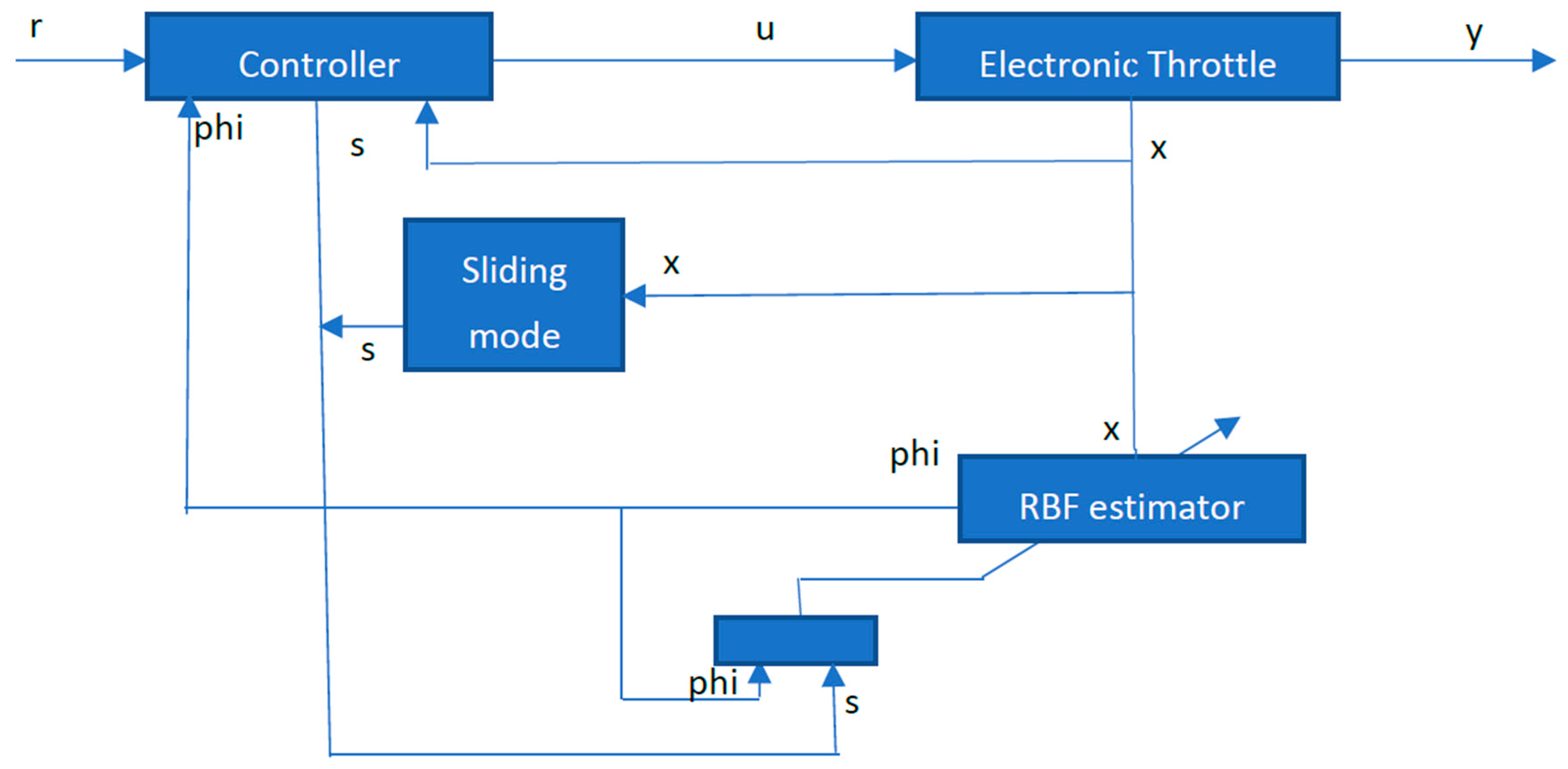Moreover, the designed control does not use the derivative of s, which avoids the singularity. The structure of the whole feedback system, including the adaptive RBF estimator, is displayed in Figure 1.

4. Fault Diagnosis and Fault Tolerant Control

As can be seen above, the output of the RBF network estimator is the derivative of the fault, thus we can easily obtain the estimation of the fault by integrating the estimator output. Here, the fourth order Runge–Kutta integration algorithm is used to reconstruct the fault signal.

$$\begin{array}{l}{k}_1=h\ast f(t_i,y_i)\\ k_2=h\ast f(t_i+\frac{h}{2},y_i+\frac{k_1}{2})\\ k_3=h\ast f(t_i+\frac{h}{2},y_i+\frac{k_2}{2})\\ k_4=h\ast f(t_i+h,y_i+k_3)\\ y_{i+1}=y_i+\frac{1}{6}(k_1+2k_2+2k_3+k_4)\end{array}$$

(32)

In this work, the RBF estimator output is not a known explicit function of time but a discrete time function only. Therefore, the function $f\left(t,y\right)$ shrinks to $f\left(t_i\right)$, and $f\left(t_i+\frac{h}{2}\right)$ takes the value of the average of the two points, $f\left(t_i\right)$ and $f\left(t_{i+1}\right)$.

Note that, in the FDI method, we generally have separate concepts and functions of fault detection to report fault occurrence, fault isolation (to isolate which fault occurs among the possible faults), fault identification (to estimate fault size and possible location), etc. With the mentioned information, the fault diagnosis is implemented. In the proposed method in this paper, the fault tolerant control is implemented straightforwardly by compensating the fault in the system dynamics, as shown in Figure 1.

It can be seen in Equation (23) that the RBF network estimate is used as part of the derivative of u₂. This is then integrated using the fourth-order Runge–Kutta algorithm in (32) to obtain u2. U2 is then involved in Equation (21) to construct the system input to control the electronic throttle tracking system. Thus, the effect caused by the fault is compensated by the estimated fault. As the weights of the adaptive RBF network are guaranteed to converge to the optimal existing weights, the adaptive wrights are bounded so that the estimated fault is also bounded. The electronic throttle system is known as an input/output stable system, thus the fault compensation does not affect the whole system stability.

5. Simulation Studies

The developed FOTSM control and adaptive RBF network estimator was applied to a simulated electronic throttle system. Matlab/Simulink based simulation studies were used to evaluate the effectiveness of the proposed method.

Step 1. A Simulink model is established for the ETS based on the model in (8)–(9) with the values of the physical parameters obtained from real experiments.

Step 2. The ETS model is put in the form of (12) with $g\left(x\right)$ and $b\left(x\right)$, as given in (10). A Matlab file is coded to present these functions with the known physical parameters of the ETS model.

Step 3. Simulate faults by changing the throttle viscous frictional torque coefficient $B_T$ and the throttle coulomb frictional torque coefficient $B_{Tf}$ as below to mimic throttle friction change.

$$B_T\left(k\right)=5B_T,B_{Tf}=0.005Nm,fork>100(t>0.1sec)$$

$$B_T\left(k\right)=2B_T,B_{Tf}=0.002Nm,fork>1100(t>1.1sec)$$

Step 4. Design the FOTSM control system. In this application, $n=2$, thus the sliding manifold in (13) is generated with ${\alpha }_1=0.3913,{\alpha }_2=0.5625,$ to satisfy (15) and ${\beta }_1=72,{\beta }_2=17$, to set the two poles at $p=-8,p=-9$, so that $p^2+{\beta }_{2}p+{\beta }_1$ is Hurwitz.

Step 5. Design the RBF network with the center, $c=\left[c_1,\dots ,c_{10}\right]=\left[\begin{array}{ccc}0.1& 0.2& \begin{array}{cc}\dots & 1.0\end{array}\\ 0.05& 0.15& \begin{array}{cc}\dots & 0.95\end{array}\\ 0.0& 0.1& \begin{array}{cc}\dots & 0.9\end{array}\end{array}\right]$, width, $\sigma =\left[{\sigma }_1,\dots ,{\sigma }_{10}\right]=\left[0.5,0.5,\dots ,0.5\right]$, and initial value of the weight $W={\left[1,1,\dots ,1\right]}^T\ast {10}^{-5}$.

Step 6. Design the control $u\left(t\right)$ according to (20), where $u_1\left(t\right)$ according to (22) and $u_2\left(t\right)$ is integrated from ${\dot{u}}_2\left(t\right)$ according to (23) using the forth-order Runge–Kutta method in (32). The control parameters in (23) are chosen as $k=6,\eta =2$.

Step 7. Design the update law of the adaptive RBF network for the weights according to (24), where the learning rate is chosen as $\gamma =10$.

Two simulations were done. In the first one, a square wave reference with different constant throttle angles were used, as shown in the second figure from the top in Figure 2, where the sliding manifold s, the two system states, the control variable u, and the applied fault are displayed from top to bottom. The fault simulated was a function of angular velocity and had a step change at time t = 0.1 sec. Then, the sliding mode variable dropped from zero. Figure 2 shows that, for the rest of the time, even in the presence of the fault, the sliding mode was forced to be zero and was maintained at zero, and therefore the first state or the output converged to the reference output, while the second state, the rotary speed, converged to zero. The dynamics of the states depended on the assigned location of poles. It was also noted that when the friction torque had significant changes, the sliding mode deviated from zero and converged to zero quickly. The output tracking was not significantly affected by the fault due to fault compensation with the RBF network. The control had no chattering due to the integration action.

The second simulation used a sinusoidal reference output to the system with the same fault applied. The fault could still be tolerated due to the function of the adaptive RBF network. While the network estimated the change rate of the fault, to compensate for the effect of the fault on the system states, the full-order terminal sliding mode control guaranteed the closed-loop system stability. It was evident that a stability guaranteed fault tolerant control was achieved. Different sizes of fault were simulated, and similar results were achieved. These results are therefore not shown here.

In order to see more clearly the effects of the fault tolerant control on rejecting fault, the part of Figure 3 involving a step change of the fault is enlarged and displayed in Figure 4. Specifically, Figure 4 displays sliding mode variable, s(t), system output tracking the reference signal, x₁(t), and fault signal changing with rotary velocity, f(t) from the time period from t = 0 to t = 0.5 s. It can be seen in Figure 4 that when the fault had a sudden change at t = 0.1 sec, the sliding mode variable s(t) was driven to deviate from zero. This caused instability in the system and performance degradation. Due to the action of the fault tolerant control, the sliding mode variable was driven back and converged to zero again, so that the system output was driven to track the reference signal without a significant influence. The adaptive RBF network was used to estimate the change rate of the fault, which was used to compensate for the fault effect in the system state equation. Thus, the post-fault system stability was guaranteed. We could also see when the tracking error changed signs, or when the system output was increased from lower than the reference signal to higher than it (or vice versa), the sliding mode generated a spike. These spikes were quickly reduced, and sliding mode returned to zero due to the control law that was derived with the Lyapunov stability theorem.

6. Conclusions

A fault tolerant tracking control system was designed in this paper with the FOTSMC and adaptive RBF estimator. The Lyapunov method was used and theoretically proved that the designed system stability is guaranteed under the post-fault dynamics. The tracking performance was maintained at a high quality with the fault effect compensated for by the adaptive RBF network estimates. The limitation that the upper bound of change rate of the fault must be known is relaxed in the proposed design. When the developed fault tolerant control method was applied to the electronic throttle tracking control, simulation results confirmed that the throttle position tracked the desired reference of the squares and the sinusoidal signal with quick response, small overshoot, and zero steady-state error. Both stability and performance were maintained after the simulated significant changes in viscous and coulomb frictions. It was evident that the developed method has great potential in industrial applications for control systems reliability improvement.