Research and Implementation of ε-SVR Training Method Based on FPGA

Abstract

Online training of Support Vector Regression (SVR) in the field of machine learning is a computationally complex algorithm. Due to the need for multiple iterative processing in training, SVR training is usually implemented on computer, and the existing training methods cannot be directly implemented on Field-Programmable Gate Array (FPGA), which restricts the application range. This paper reconstructs the training framework and implementation without precision loss to reduce the total latency required for matrix update, reducing time consumption by 90%. A general ε-SVR training system with low latency is implemented on Zynq platform. Taking the regression of samples in two-dimensional as an example, the maximum acceleration ratio is 27.014× compared with microcontroller platform and the energy consumption is 12.449% of microcontroller. From the experiments for the University of California, Riverside (UCR) time series data set. The regression results obtain excellent regression effects. The minimum coefficient of determination is 0.996, and running time is less than 30 ms, which can meet the requirements of different applications for real-time regression.

1. Introduction

Support Vector Regression (SVR) belongs to a classic application in Support Vector Machine (SVM) [1]. It has been widely used in the fields of sample regression [2], data prediction [3], fault diagnosis [4] and so on. The existing libraries for implementation of SVR, such as SVM Light and LibSVM, need to be run based on personal computers. These methods focus on the application of SVR and do not consider the underlying design of the software. With the increasing use of embedded artificial intelligence in various fields, there is an urgent need for a platform with small size, high performance, and low power consumption. Commonly used embedded artificial intelligence platforms include Advanced RISC Machine (ARM) and Field-Programmable Gate Array (FPGA). ARM-based SVR depends on the performance of hardware kernel. The development of SVR based on bare metal is difficult and time-consuming. High performance kernels usually support embedded systems with complex peripheral circuits, high power consumption and costs. All of these restrict the application of SVR in ARM. Compared with ARM, FPGA has obvious advantages, such as high flexibility, simple hardware circuit, and low power consumption. The implementation of SVR using FPGA has attracted a large number of researchers. Noronha et al. proposes a parallel FPGA implementation of the Sequential Minimal Optimization (SMO) of SVM [5]. After the parallel implementation, SVM is validated by bit-accurate simulation. Meanwhile, Lopes et al. realize parallel implementation of SVM using Stochastic Gradient Descent (SGD) algorithm on FPGA [6]. In order to model the implied volatility surface, Yaxiong Zeng et al. implement most computationally intensive parts in a FPGA, where a 132× speedup is achieved during online prediction [7]. Matrix product is the key step in SVM, and a novel matrix-vector product approach is proposed in [8].

The training method of SVR is similar to that of SVM, thus the research on SVM is also applicable to SVR. The implementation of SVM is divided into two parts: forward inference and training. For the research of forward inference on FPGA, a high performance, low resource consuming hardware design for Support Vector Classification (SVC), and SVR is proposed in [9]. This system is implemented on a low cost FPGA and exploits the advantages of parallel processing to compute the feed forward in SVM. The method of cascade SVM in [10] is used to implement face recognition on FPGA. In [11] the authors propose a parallel hardware architecture for target detection, which applies SVM to real-time detection of targets such as faces, pedestrians, and vehicles. A low-complexity pedestrian detection framework is proposed in [12] for intelligent video surveillance systems. Jian Hua Luo et al. [13] combined SVM and Histogram of Oriented Gradient (HOG) to realize real-time pedestrian detection system design on FPGA with a small amount of resources. Early research emphasized the processing of kernel functions and the implementation of parallel computation of multiple input data and achieved significant acceleration effects. The detection object in the above applications is a fixed model. Usually the training of model is achieved through a computer, and then the model should be imported into FPGA. Therefore, if the model changes, the new model needs to be retrained on the computer to get new training parameters. In order to adapt to changes in the model, the accelerated training method based on FPGA has caused widespread concern. Papadonikolakis et al. focus on the acceleration of training phase and a geometric approach to SVM training based on Gilbert’s Algorithm is targeted, due to the high parallelization potential of the heavy computational tasks [14]. Cao Kui Kang et al. proposed a parallel scalable digital architecture of SMO, which realized online training of SVM based on FPGA [15]. The test is performed using sonar data with a maximum classification error of 8.65%. This method provides guidance for online training of SVM. For the key steps of SMO to satisfy Karush–Kuhn–Tucher (KKT) conditions during training, Jhing-Fa Wang et al. studied the implementation of SMO, which includes Intellectual Property (IP) core implementation of SMO [16], an efficient configurable chip design based on SMO acceleration training method [17], and implementation of a low cost trainable SMO mode classifier [18]. The above research adopts a development method close to the underlying layer. It still requires a lot of manpower and time. In order to reduce the FPGA-based development cycle, Afifi et al. implemented the SVM classifier for online detection of skin cancer based on Zynq platform, and the system power consumption is less than 1.5 W [19,20]. Hongda Wang et al. proposed a real-time seizure detection hardware design based on STFT for nonlinear SVM [21]. The experiment achieves a 1.7× improvement, and the total power is less than 380 mW. Tsoutsouras V uses Vivado High-Level Synthesis (HLS) to implement hardware acceleration of SVM for electrocardiogram arrhythmia detection, achieving 78× acceleration compared to software execution [22]. Based on the Zynq platform, Benkuan Wang et al. used the Least Squares Support Vector Machine (LSSVM) for online fault diagnosis of an Unmanned Aerial Vehicle (UAV) [23,24]. The Vivado HLS accelerated kernel matrix and inversion processing of LSSVM to realize data prediction and state judgment. The above research provide new ideas for hardware implementation of SVM/SVR. To our best knowledge, the existing literature does not have a systematic research and implementation of ε-SVR training method based on FPGA. Therefore, this paper studies the implementation of ε-SVR training method based on FPGA. The main contributions of this paper are as follows:

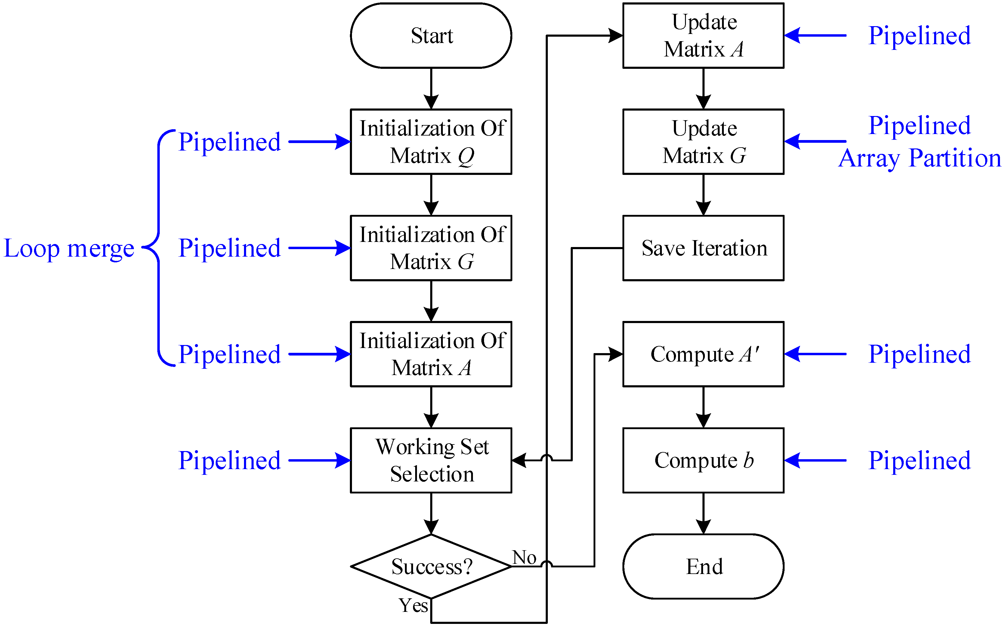
(1) In view of the complexity of the existing training method, this paper reconstructs the training framework and implementation without precision loss to reduce the total latency required for matrix update.

(2) Based on the parallel characteristics of FPGA, this paper uses the techniques of pipeline and array partition to optimize the execution of ε-SVR. A small amount of resource consumption in exchange for a significant increase in performance.

(3) A general ε-SVR training system with low latency is implemented on Zynq platform, software and hardware co-design makes this system suitable for different regression scenarios with low power consumption and high performance.

The rest of the paper is organized as follows: Section 2 describes the principles and hardware design of ε-SVR. Section 3 uses Vivado HLS to accelerate the implementation of ε-SVR based on FPGA. Section 4 describes the experimental results and compares with other platforms. Section 5 summarizes this paper and presents future work.

2. Hardware Reconstruction of ε-SVR

2.1. Principle of ε-SVR

The purpose of ε-SVR training method is to solve the regression function in a given sample space. The maximum error between predicted value and true value is less than ε. It is assumed that the samples used for regression belong to the data set shown in Equation (1), wherein the number of samples is l, each sample x_i belongs to the space of dimension d, and y_i is the true value in one-dimensional space.

This paper takes the regression of samples in two-dimensional space as an example, as shown in Figure 1. Equation (2) is used to represent the regression function f(x) obtained from training, where x is the input samples, w is the coefficient of the regression function, <w,x> is the kernel function, and b is the bias. The ε-SVR training method consists of determining the function f(x) and optimizing the solution to minimize the expected risk.

$$\left\{\left(x_1,y_1\right),\left(x_2,y_2\right),\dots ,\left(x_l,y_l\right)|x_i\in X=R^d,y_i\in Y=R,i=1,\dots ,l\right\}$$

(1)

$$f\left(x\right)=\langle w,x\rangle +b,w\in X,b\in R.$$

(2)

According to [25], the optimization problem is expressed in Equation (3):

$$\begin{array}{l}min\hspace{1em}\hspace{1em}\hspace{1em}\frac{1}{2}{\Vert w\Vert }^2\\ subject to \{\begin{array}{l}{y}_i-\langle w,x\rangle -b\le \epsilon \\ \langle w,x\rangle +b-y_i\le \epsilon \end{array}\end{array}$$

(3)

By constructing the Lagrange equation to solve the inequality constraint problem in Equation (3), Equation (4) represents the optimal solution problem S, where K represents the matrix constructed by kernel function and A represents the Lagrange multiplier.

$$\{\begin{array}{l}S=min\left\{\frac{1}{2}AQ{A}^T+\left[\begin{array}{cc}\epsilon -y& \epsilon +y\end{array}\right]A^T\right\}\\ Q=\left[\begin{array}{cc}K& -K\\ -K& K\end{array}\right]=K\left[\begin{array}{cc}1& -1\\ -1& 1\end{array}\right]\\ A=\left[\begin{array}{cc}\alpha & {\alpha }^{*}\end{array}\right]\end{array}.$$

(4)

The coefficient w and bias b of the regression function are processed by solving the Langrage multiplier in Equation (4), and the regression function f(x) after training is expressed by the Equation (5). The kernel function type used in the following sections is Radial Basis Function (RBF), and the expression is shown in Equation (6).

$$\{\begin{array}{l}f\left(x\right)={\displaystyle \sum _{i=1}^l\left({\alpha }_i-{\alpha }_i^{*}\right)\varphi \left(x_i\right)\varphi \left(x\right)}+b={\displaystyle \sum _{i=1}^l{A}_i\prime K\left(x_i,x\right)}+b\\ A\prime =\alpha -{\alpha }^{*}\end{array},$$

(5)

$$\varphi \left(x_i\right)\varphi \left(x\right)=e^{-\gamma {\Vert x_i-x\Vert }^2}.$$

(6)

For the solution of the optimization problem in Equation (4), the commonly used method include SMO [5], SGD [6], etc. The SMO only needs to update two parameters in each iteration, which has the characteristics of small calculation amount and high precision. Therefore, it is widely used in the training method of ε-SVR. This paper refers to the training method of SMO designed in [25]. The symbol matrix e and the gradient matrix G are initialized with Equation (7).

$$\{\begin{array}{l}e=\left[\begin{array}{cc}\underset{l}{\underbrace{1\cdots 1}}& \underset{l}{\underbrace{-1\cdots -1}}\end{array}\right]\\ G=\left[\begin{array}{cc}\epsilon -y& \epsilon +y\end{array}\right]\end{array}.$$

(7)

The indices of matrix for updating in the SMO are determined according to the working set selection proposed in [25]. Assuming that the indices of selected matrices are i and j, the corresponding matrices A_i and A_j of Lagrange multiplier are updated using Equation (8). The updated results should be limited between the upper (H) and the lower (L), as shown in Equation (9).

$$\{\begin{array}{l}{A}_i^{new,un}=A_i^{old}-\frac{G_i+e_i{e}_j{G}_j}{Qua{d}_{i,j}}\\ A_j^{new,un}=A_j^{old}-\frac{G_j-e_i{e}_j{G}_i}{Qua{d}_{i,j}}\\ Qua{d}_{i,j}=K_{i,i}+K_{j,j}-2K_{i,j}\end{array},$$

(8)

$$A^{new}=\{\begin{array}{l}H\\ A^{new,un}\\ L\end{array},\begin{array}{c}{A}^{new,un}>H\\ L\le A^{new,un}\le H\\ A^{new,un}>L\end{array}.$$

(9)

The gradient matrix is updated using Equation (10) to complete a single iteration based on SMO while preparing for the next working set selection. In the next iteration of working set selection, if the maximum difference between the gradient matrix is less than the maximum error ε, it indicates that the current training result satisfies the KKT condition, while the iterative training ends.

$$\{\begin{array}{l}{G}_k^{new}=G_k^{old}+Q_{i,k}\Delta A_i+Q_{j,k}\Delta A_j\\ \Delta A_i=A_i^{new}-A_i^{old}\end{array}.$$

(10)

Through above analysis of the ε-SVR training method, the training process based on SMO mainly includes working set selection and the update of matrix. The Lagrange multiplier matrix processed after the training is used to derive coefficient w and bias b. Thereby the solution of regression function is realized. The optimized hardware design of training method will be implemented in the next section.

2.2. Hardware Design of ε-SVR

Implementation of ε-SVR consists of two parts: iterative training and inferential regression. The design of inference regression is similar to the implementation of SVM. Our team discussed the implementation of the SVM in [26]. This paper focuses on the hardware design of the training method. According to the previous analysis, the training method is an iterative process focusing on the iterative update of Lagrange multiplier and gradient matrix. As shown in Figure 2, the matrix is updated by direct hardware mapping method. The operations include addition, subtraction, multiplication, division, exponential, and comparison. The types of operations are all floating point. Data operations required for a single iteration of matrix update are shown in

Table 1. Direct hardware mapping operation statistics.

Arithmetic	Operations	Maximum Latency
Addition	7	8
Subtraction	11	8
Multiplication	38	8
Division	2	28
Exponential	5	29
Comparison	4	2

. According to the parameters provided in Vivado, the maximum latency corresponding to different operations is listed in Table 1. The direct hardware mapping method used in Figure 2 requires the construction of multiple floating-point arithmetic units. Assuming that the extra time consumption caused by data transfer is not considered, the total latency required for update is 657. Therefore, if the direct hardware mapping is adopted, the problems such as large amount of processing, high resource consumption, and slow efficiency will occur.

In order to solve the problems caused by direct hardware mapping, the mapping process of training needs to be improved. The optimization strategies adopted in this paper include the optimization of training framework and implementation. According to the contents of Table 1, the multiplication is the most frequent process, and division and exponential cause the largest latency. As shown in Figure 2, the process of kernel function occupies all the exponential operations and most of the multiplication operations, which are the processes of matrix Q in Equation (4) and matrix Quad in Equation (8). By constructing the kernel matrix, the processing of kernel function in the original framework is eliminated. It can be known from Equation (4) that the matrix Q is a symmetric matrix constructed by kernel matrix with different coefficients. Considering that direct construction will consume a large amount of storage resources, this paper replaces the matrix Q with kernel matrix by the strategy of address indirect mapping. In the optimization of the implementation, according to Equation (7), the value of the matrix e is 1 or −1. However, matrix e only participates in multiplication in Equation (8), so this paper replaces the original framework with hardware operation of xor to simplify the implementation. The optimized hardware mapping block diagram is shown in Figure 3. The statistics of operations in Figure 3 are shown in

Table 2. Optimized hardware mapping operation statistics.

Arithmetic	Operations	Maximum Latency
Addition	2	8
Subtraction	5	8
Multiplication	2	8
Division	2	28
Exponential	0	29
Comparison	4	2

. Since the process of kernel function is not required in the matrix update, the operation of exponential is reduced to zero. At the same time, the operations of multiplication are greatly reduced, and the operations of addition and subtraction are reduced by a small amount. The division and comparison belong to the main process of matrix update, which remains unchanged. Through the above optimization strategy, the total latency required for matrix update is reduced to 136, and the amount of operations and resource consumption are reduced. Then the efficiency of proposed framework is improved.

According to the optimized hardware mapping method, the ε-SVR training is divided into three parts: matrix initialization, iterative optimization (SMO Solver), and regression function processing. The software flow chart of ε-SVR training designed in this paper is shown in Figure 4. The initialization module includes the initialization of gradient matrix G, Lagrange multiplier A, the kernel matrix Q. The iterative optimization implements SMO, including working set selection and optimized matrix update. In the design of this paper, a statistics function is added to record the number of iterations. The processing of regression function is mainly dealt by deriving the coefficient w and bias b.

ε-SVR has no limitation on the dimensions of the training samples. The difference of input data with different dimensions in the training lies in the processing of kernel matrix, and the subsequent SMO remains unchanged. In order to verify the effect of the proposed ε-SVR training method, this paper takes the curve regression of discrete samples in two-dimensional plane as an example. The coefficient of determination (R²) is used to measure the regression effect [27]. The expression of R² is shown in Equation (11), where f_i is the predicted value of regression function with input value x_i.

$$\{\begin{array}{l}\overline{y}=\frac{1}{l}{\displaystyle \sum _{i=1}^l{y}_i}\\ R^2=1-\frac{{\displaystyle \sum _{i=1}^l{\left(y_i-f_i\right)}^2}}{{\displaystyle \sum _{i=1}^l{\left(y_i-\overline{y}\right)}^2}}\end{array}.$$

(11)

Since the predicted value of regression function deviates from true value, the larger the deviation, the smaller coefficient of determination. Under the ideal condition, the deviation between predicted value and true value is zero, and R² is equal to 1, which is the optimal regression effect.

Figure 5 is the regression diagram of the ε-SVR training method proposed in this paper, including input samples and regression curve. The coefficient of determination calculated by Equation (11) is 0.970. The result shows that the training method completes the regression of given samples and achieves a good regression effect.

3. Acceleration Unit Design of ε-SVR

In applications where real-time regression is required, a single system needs to perform multiple sets of data for online training at the same time. The traditional pipelined processor cannot meet the requirements of the system while FPGA has the ability to process multiple sets of data in parallel. This paper chose to use Xilinx Zynq platform, which is divided into Process System (PS) and Program Logic (PL) in chip. This platform meets the requirements of high performance and parallelism. The Vivado HLS tools convert the original algorithm into Hardware Description Language (HDL), deploying it in the form of a custom core on PL, and PS transfers data and controls the running state of custom core through the Advanced eXtensible Interface (AXI) bus. Compared with the traditional development method, it not only saves development time, but also accelerates the implementation of training method efficiently.

The FPGA-based ε-SVR acceleration system designed in this paper is shown in Figure 6. The Application Processor Unit (APU) with dual-core Cortex-A9 in PS serves as the central controller in this system. The Central Interconnect acts as a bridge between the APU and other modules to transmit control commands. PL to Memory Interconnect is connected to Memory Interfaces for accessing external memory. The external memory used in this system is Double Data Rate 3 (DDR3) Synchronous Dynamic Random Access Memory (SDRAM). In order to reduce the usage rate of APU during sample data transmission, this system builds the Direct Memory Access (DMA) controller and an acceleration unit of ε-SVR on PL. The design proposed in this paper also supports the construction of multiple acceleration units. DMA controller automatically transfers the samples to the acceleration unit. After the acceleration unit completes the training of samples, results are selected to be stored in the PL or external memory according to the requirements of application.

In the implementation of acceleration unit of ε-SVR based on FPGA, the definition of input and output interfaces needs to be completed firstly. It can be known from Equation (1) that the input data include the values of X and Y. The parameters to be defined in the training process include C and ε. C is the cost factor, which indicates tolerance to the error and affects the regression effect after training. ε determines the width of the insensitive area of samples, which affects the number of support vectors. It is closely related to the noise of samples in the application. An additional parameter γ needs to be defined if the type of kernel function is RBF. It determines the data distribution when the samples are mapped to the high-dimensional feature space, which reflects the degree of relaxation between samples. It directly affects the number of iterations during the training process. From the above analysis, the complexity and generalization ability of training model depend on these parameters. The acceleration unit is started after the completion of transmission. After iterative training of acceleration unit, matrix A′ and b are selected as results, which are the regression function f(x). The number of iterations is outputted as optional information.

The workflow of proposed system is as follows. The APU in PS is connected to the General Purpose (GP) port through the Central Interconnect, which is connected to the DMA controller and the acceleration unit using AXI4-Lite bus. The direction of arrow in Figure 6 indicates the master-slave relationship between buses. The parameters of DMA controller include the address and length of matrix X and Y. DMA controller reads the samples stored in the external memory through the High Performance (HP) port with AXI4-Memory Map bus mode. The data stream is transmitted to the acceleration unit using AXI4-Stream mode to ensure the correctness of transmission. The acceleration unit reads the samples transferred by the DMA and completes the data initialization (Q, Quad, and G) in combination with the parameters (C, ε, and γ), and then it proceeds the module of SMO Solver to solve the matrix A and G until the parameters satisfy the KKT condition. Finally, the matrices A′ and b are computed by the matrix A. For the design of storage mode of matrix A′, this system refers to the methods in [19] and [20]. The results are stored in the external memory under the condition of large sample data, thereby saving on-chip resources. Meanwhile, if small samples are used, the acceleration unit stores the results directly in the on-chip Block Random Access Memory (BRAM), which facilitates the re-reading of acceleration unit during prediction.

During the design of the acceleration unit, in order to make full use of the parallel characteristics of FPGA, it is necessary to optimize and accelerate the training method reconstructed in the previous description at the hardware layer, which reduces running time without precision loss. This paper uses the following strategies to accelerate the training.

3.1. Single Loop Optimization

There is a large amount of loop processing on matrix in training, such as the assignment of matrix in the data initialization and the update of matrix in SMO. Figure 7 is the schematic diagram of Loop Pipelining optimization for a single loop. A single loop contains reading, computing, and writing of data. The traditional processing method only performs one operation in one clock cycle. Therefore, it takes at least eight clock cycles to complete three loops. This paper uses pipelining to optimize the execution of the loop. Thus, the data can be written, computed, and read simultaneously during processing, which improves the bandwidth of the data storage and the effective utilization.

3.2. Nested Loop Optimization

In addition to single loop optimization described above, there are also a large number of nested loops in the proposed method. The type of kernel function matrix is two-dimensional, and the initialization needs to be done by nested loops. As shown in Figure 8, the nested loop optimization diagram is different from single loop optimization. The second execution of the inner loop needs to re-establish a new memory read and write operation. During the re-execution of inner loop, the memory access has an idle period for rewinding the address from end to start. Therefore, this paper adopts the rewinding strategy. As shown in Figure 9, after the inner loop is completed, the idle period is eliminated by pre-reading the data of the next loop in advance. The optimization can effectively improve the efficiency of nested loop, especially as the iteration of inner loop is frequent and it needs to be executed multiple times.

3.3. Array Partition Optimization

The pipelined optimization is used to improve the bandwidth usage of existing memory block, but the bandwidth of on-chip memory becomes a bottleneck limiting the execution efficiency of training. From the analysis of the SMO in [5], the length of the matrix G is twice the number of samples. Usually the matrix is stored in a single BRAM, and only one element of matrix can be updated in a single cycle. In view of the fact that the matrix G needs to be updated twice, this paper adopts the strategy of array partitioning to improve the parallelism of training. As shown in Figure 10, a partition optimization diagram is performed. Compared with no optimization, the optimized design performs two matrix processing at the same time, and the number of cycles required is half of the original, which improves the execution efficiency of the design.

3.4. Other Optimizations

In addition to the optimization strategies proposed above, others are also used to accelerate training. Multiple matrices are initialized simultaneously using the loop merge method during the data initialization stage. In the [26], adding FIFO to the AXI4-Memory Map improves the ability of DMA to read data. Inline instructions are used in Vivado HLS to reduce the time of function calls.

The original training method is accelerated according to the optimization strategy proposed above. Figure 11 shows a flow chart with optimized annotations. Since each stage of training execution includes loop processing of matrix data, the loop pipelining optimization is applied to each stage of the flowchart, and the loop pipelining with rewind optimization is used for the nested loop. Since optimization of array partition is closely related to the type of matrix, it is suitable for the update of gradient matrix G. The loop merge optimization combines multiple unrelated loops and it is suitable for the data initialization of acceleration unit.

Vivado HLS report with latency is used to evaluate the optimization results. This paper divides optimization into four levels, namely the Original (-O0), Pipelined (-O1), Array Partition (-O2), and Loop Merge (-O3). The test results are shown in

Table 3. Latency at different optimization levels.

	Data_Init	SMO Solver	A’	b	Total
-O0	85,492	1400~35,890,003	325	730~742	97,969~35,976,562
-O1	65,107	352~3,590,003	52	333~345	65,844~3,655,507
-O2	65,064	312~3,190,003	52	333~345	65,761~3,255,464
-O3	65,022	312~3,190,003	52	333~345	65,719~3,255,422

. Compared with original, pipelining optimization reduces the latency of each module. Array partition reduces the time in data initialization and SMO Solver, while loop merge reduces the latency of data initialization. Since optimization level ‘-O3’ has minimal latency, it is used in subsequent experiments. In the next section, the acceleration system is implemented on the experimental platform.

4. Experimental Results and Evaluation

The experimental platform used in this paper is XC7Z020CLG484-1 and the acceleration system in Figure 6 is implemented in Vivado. According to the previous description of the optimization of ε-SVR, the acceleration unit with different optimization levels (-O0, -O1, -O2, and -O3) is constructed. Resource, power, and running time are evaluated with other platforms. Finally, the partial dataset from the University of California, Riverside (UCR) time series is used to test the regression effect and verify the real-time performance.

4.1. Comparison of Resource Utilization

Figure 12 shows the resource utilization at different optimization levels.

Table 4. Resource utilization at level ‘-O3’.

Resource	Utilization	Available	Percentage (%)
LUT	16,684	53,200	31.36
LUTRAM	582	17,400	3.34
FF	18,632	106,400	17.51
BRAM	10.5	140	7.50
DSP	71	220	32.27

lists the detailed resource utilization at the optimal level. According to Figure 12, resource utilization of no optimization is minimal among different levels. After the optimization of the -O1 level, the consumption ratios of Look-Up-Table (LUT), Flip Flop (FF), and Digital Signal Processing (DSP) increase slightly, while the consumption ratios of LUTRAM and BRAM vary little. In the following optimization, in addition to the large proportion of DSP, the others remain almost unchanged. Compared with the original design, the increase in the proportion of DSP intensifies the computational power. In the resource consumption corresponding to the -O3 optimization level, DSP remains unchanged, but the consumption ratios of LUT and LUTRAM are decreased. It shows that the architecture of acceleration unit is improved, and the occupied resources have been released while maintaining the efficiency of original. As can be seen from the detailed resource utilization in Table 4, the largest consumption ratio in this system is 32.27%. According to the parallel characteristics of FPGA, additional acceleration units can be constructed to further improve the computing ability of the single chip.

The power consumption of the embedded system is also an important indicator. The embedded system typically has lower power consumption, allowing it to keep working for a long time in special applications.

Table 5. System power consumption.

Total	2.037 W	ε-SVR	0.343 W	Clocks	0.068 W
				Signals	0.124 W
				Logic	0.097 W
				BRAM	0.012 W
				DSP	0.041 W
		PS7			1.531 W
		PL Static			0.164 W

shows the statistics table with system power consumption. The total power consumption is 2.037 W, of which PS7 consumes the most power. The ε-SVR acceleration unit consumes 0.343 W, and it is much smaller than PS7. If only the acceleration unit is running in this system, the power consumption of PS7 can be omitted. In addition, during the test, the default frequency of the Cortex-A9 core is 667 MHz, and lower power consumption (1.313 W) is achieved by reducing the core frequency (50 MHz).

In order to evaluate the rationality of the system’s resource distribution, this paper uses Xilinx Implemented Design in Vivado to obtain on-chip place and route. Different colors are used to mark the distribution of different modules, as shown in Figure 13. This design has a better uniformity within the constraint region. However, since the kernel function of the RBF type is used in this paper, there are exponential type floating-point operations in matrix initialization, thus the matrix initialization module shown in Figure 13 occupies a large amount of resources.

4.2. Comparison of Running Time

In this paper, the sample data in Figure 5 is used to test the running time of the ε-SVR acceleration. The running time at different optimization levels is shown in

Table 6. Running time at different optimization levels.

Optimization	Time (ms)
-O0	108.527
-O1	16.219
-O2	14.449
-O3	14.445

. Compared with the original, the optimization of the -O1 level significantly improves the performance, and other levels of optimization further reduce the running time. Experimental results are in agreement with the report in Table 3. Meanwhile, the running time is reduced to 13.31% compared with the original, which has an obvious acceleration effect.

Combined with the existing test equipment in our lab, this paper uses the STM32 series of microcontrollers from STMicroelectronics to compare the running time of training. The parameters of selected microcontrollers are shown in

Table 7. Performance with different platforms.

	STM32F469	STM32F767	XC7Z020		XCZU9EG
			PS	PL	PS	PL
FPU	Single	Double	Double	Single 1	Double	Single 1
Kernel Type	Cortex-M4	Cortex-M7	Cotrtex-A9	FPGA	Cortex-A53	FPGA
Frequency (MHz)	180	216	667	100	1300	200
Optimization	Speed	Speed	Speed	-O3	Speed	-O3
Time (ms)	205.007	136.810 2	30.581	14.445	14.623	7.589
Power (W)	0.339	0.411	1.531	0.507	2.667	1.140
Energy (mJ)	69.492	56.229	46.820	7.324	39.000	8.651

¹ The precision type of floating point IP core is single. ² The cache of kernel is valid.

. The PS of Zynq is capable of running a bare metal program with Xilinx SDK (Software Development Kit, 2016.4, Xilinx, San Jose, CA, USA, 2016). This paper also tests the performance of the proposed algorithm in PS. In the embedded field, energy efficiency ratio is an important factor in estimating power consumption, which is the energy consumed to perform the training method with different platforms. Therefore, the energy consumed with different platforms is listed in the last row of Table 7. It is worth noting that the low-frequency of kernel has a lower power, but the corresponding processing time is longer than high-frequency and it cannot compensate for the increase in power consumption. Therefore, the experimental results in this paper only compare the best energy consumption achieved by the kernel at the highest frequency. The optimization flag of compiler is also an important factor affecting the efficiency of the algorithm. The speed-first compilation flag is used to get the optimal running result.

When we use the frequency of acceleration unit at 200 MHz in our experiments, due to problems such as the speed level of hardware, the report from Vivado HLS points out that an additional latency is needed to maintain the stability of acceleration unit. That is to say, the increase in frequency does not satisfy the extra consumption of latency. Therefore, this paper uses a new platform (ZCU102) with higher speed level. The parameters are shown in the last column of Table 7. Using the same optimization level, a new acceleration system is built on this platform. The frequency of acceleration unit is updated to 200 MHz. Experimental result shows that the running time is reduced from 14.445 to 7.589 ms. Thus, the platform with a higher speed level can further improve the performance of the acceleration unit. It can be seen from Table 7 that the running time of Cortex-M4 with the Float Point Unit (FPU) is the longest among results. The running time is greatly improved with the increase of the frequency of kernel. The test platform of Cortex-A53 kernel (1300 MHz) achieves optimal running time with the result of 14.623 ms. As can be seen from the results, the method of increasing the frequency of kernel to reduce the energy is limited, because high-frequency has more static power consumption, thus this method is not suitable for the application requiring low power. The implementation of algorithm based on FPGA reduces the energy under the premise of achieving the same performance, and the energy consumed by PL in XC7Z020 is 18.779% of PS in XCZU9EG. Compared with the platform of microcontroller, the maximum acceleration ratio is 27.014x, and the corresponding energy is 12.449% of the former. Thus, the implementation of the algorithm in this paper has higher performance and better energy consumption.

4.3. Regression Results of UCR Time Series Dataset

In this paper, two-dimensional random samples in Figure 5 were used in the previous test. In order to verify the test results of real data, this paper selects six samples from the UCR time series dataset to verify the regression effect and time consumption [28]. Figure 14 shows the samples in different types of time series datasets and the regression curves obtained by the proposed training method, where the x coordinate of samples is normalized. The training parameters, number of iterations, time consumption, and coefficient of determination are noted in Figure 14. It can be seen from the experiments for the selected time series samples that the regression results of the acceleration unit obtain an excellent regression effects, and the minimum coefficient of determination is 0.996. The time consumption is less than 30 ms, which can meet the requirements of different applications for real-time regression.

5. Conclusions

In this paper, the training method of ε-SVR based on FPGA was studied. The strategy was adopted to optimize the training framework and implementation. The acceleration unit design of ε-SVR was also optimized in combination with the parallel characteristics of FPGA. Experimental results show that the acceleration unit designed in this paper has an obvious acceleration effect, and time consumption reduced to 13.31% without precision loss. Compared with the microcontroller platform, the maximum acceleration ratio reaches 27.014× and the energy consumption is 12.449% of the microcontroller. Additional experimental results of UCR time series dataset show that the acceleration system has an excellent data regression effect for different types of time series, and the running time is less than 30 ms, which can meet the real-time requirements in different applications. However, there are also deficiencies in this design. The processing of the kernel function in the acceleration unit consumes a large amount of on-chip resources, resulting in a low resource utilization rate for the SMO module. In the future, large-scale samples require a large amount of memory resources to hold the kernel matrix. It is a significant factor affecting resource utilization. Synchronous processing of the kernel matrix is the key step in achieving SVR training method for large-scale samples, which needs to be further studied.

References

1. Chang, C.; Lin, C. LIBSVM: A library for support vector machines. ACM Trans. Intell. Syst. Technol. (TIST) 2011, 2, 1–27. [Google Scholar] [CrossRef]
2. Karimipour, A.; Bagherzadeh, S.A.; Taghipour, A.; Abdollahi, A.; Safaei, M.R. A novel nonlinear regression model of SVR as a substitute for ANN to predict conductivity of MWCNT-CuO/water hybrid nanofluid based on empirical data. Phys. A Stat. Mech. Appl. 2019, 521, 89–97. [Google Scholar] [CrossRef]
3. Vrablecová, P.; Bou Ezzeddine, A.; Rozinajová, V.; Šárik, S.; Sangaiah, A.K. Smart grid load forecasting using online support vector regression. Comput. Electr. Eng. 2018, 65, 102–117. [Google Scholar] [CrossRef]
4. Zahid, M.; Ahmed, F.; Javaid, N.; Abbasi, R.; Zainab Kazmi, H.; Javaid, A.; Bilal, M.; Akbar, M.; Ilahi, M. Electricity Price and Load Forecasting using Enhanced Convolutional Neural Network and Enhanced Support Vector Regression in Smart Grids. Electronics 2019, 8, 122. [Google Scholar] [CrossRef]
5. Noronha, D.H.; Torquato, M.F.; Fernandes, M.A.C. A parallel implementation of sequential minimal optimization on FPGA. Microprocess. Microsyst. 2019, 69, 138–151. [Google Scholar] [CrossRef]
6. Lopes, F.F.; Ferreira, J.C.; Fernandes, M.A.C. Parallel Implementation on FPGA of Support Vector Machines Using Stochastic Gradient Descent. Electronics 2019, 8, 631. [Google Scholar] [CrossRef]
7. Zeng, Y.; Klabjan, D. Online adaptive machine learning based algorithm for implied volatility surface modeling. Knowl.-Based Syst. 2019, 163, 376–391. [Google Scholar] [CrossRef]
8. Pan, J.; Lee, C.; Sghaier, A.; Zeghid, M.; Xie, J. Novel Systolization of Subquadratic Space Complexity Multipliers Based on Toeplitz Matrix–Vector Product Approach. IEEE Trans. Very Larg. Scale Integr. (VLSI) Syst. 2019, 27, 1614–1622. [Google Scholar] [CrossRef]
9. Ruiz-Llata, M.; Guarnizo, G.; Yébenes-Calvino, M. FPGA implementation of a support vector machine for classification and regression. In Proceedings of the International Joint Conference on Neural Networks (IJCNN), Barcelona, Spain, 18–23 July 2010; IEEE: Piscataway, NJ, USA, 2010; pp. 1–5. [Google Scholar]
10. Kyrkou, C.; Bouganis, C.; Theocharides, T.; Polycarpou, M.M. Embedded Hardware-Efficient Real-Time Classification With Cascade Support Vector Machines. IEEE Trans. Neural Netw. Learn. Syst. 2016, 27, 99–112. [Google Scholar] [CrossRef]
11. Kyrkou, C.; Theocharides, T. A parallel hardware architecture for real-time object detection with support vector machines. IEEE Trans. Comput. 2012, 61, 831–842. [Google Scholar] [CrossRef]
12. Bilal, M.; Khan, A.; Khan, M.U.K.; Kyung, C. A Low-Complexity Pedestrian Detection Framework for Smart Video Surveillance Systems. IEEE Trans. Circuits Syst. Video Technol. 2017, 27, 2260–2273. [Google Scholar] [CrossRef]
13. Luo, J.; Lin, C. Pure FPGA Implementation of an HOG Based Real-Time Pedestrian Detection System. Sensors 2018, 18, 1174. [Google Scholar] [CrossRef] [PubMed]
14. Papadonikolakis, M.; Bouganis, C.S.; Constantinides, G. Performance comparison of GPU and FPGA architectures for the SVM training problem. In Proceedings of the International Conference on Field-Programmable Technology, Sydney, NSW, Australia, 9–11 December 2009; IEEE: Piscataway, NJ, USA, 2009; pp. 388–391. [Google Scholar] [Green Version]
15. Cao, K.K.; Shen, H.B.; Chen, H.F. A parallel and scalable digital architecture for training support vector machines. J. Zhejiang Univ. Sci. C 2010, 11, 620–628. [Google Scholar] [CrossRef]
16. Kuan, T.; Wang, J.; Wang, J.; Lin, P.; Gu, G. VLSI Design of an SVM Learning Core on Sequential Minimal Optimization Algorithm. IEEE Trans. Very Large Scale Integr. (VLSI) Syst. 2012, 20, 673–683. [Google Scholar] [CrossRef]
17. Peng, C.; Chen, B.; Kuan, T.; Lin, P.; Wang, J.; Shih, N. REC-STA: Reconfigurable and Efficient Chip Design With SMO-Based Training Accelerator. IEEE Trans. Very Large Scale Integr. (VLSI) Syst. 2014, 22, 1791–1802. [Google Scholar] [CrossRef]
18. Peng, C.; Kuan, T.; Lin, P.; Wang, J.; Wu, G. Trainable and Low-Cost SMO Pattern Classifier Implemented via MCMC and SFBS Technologies. IEEE Trans. Very Large Scale Integr. (VLSI) Syst. 2015, 23, 2295–2306. [Google Scholar] [CrossRef]
19. Afifi, S.; GholamHsosseini, H.; Sinha, R. Dynamic hardware system for cascade SVM classification of melanoma. Neural Comput. Appl. 2018, 30, 1–12. [Google Scholar] [CrossRef]
20. Afifi, S.; GholamHosseini, H.; Sinha, R. A system on chip for melanoma detection using FPGA-based SVM classifier. Microsystems 2019, 65, 57–68. [Google Scholar] [CrossRef]
21. Wang, H.; Shi, W.; Choy, C. Hardware Design of Real Time Epileptic Seizure Detection Based on STFT and SVM. IEEE Access 2018, 6, 67277–67290. [Google Scholar] [CrossRef]
22. Tsoutsouras, V.; Koliogeorgi, K.; Xydis, S.; Soudris, D. An Exploration Framework for Efficient High-Level Synthesis of Support Vector Machines: Case Study on ECG Arrhythmia Detection for Xilinx Zynq SoC. J. Signal Process. Syst. 2017, 88, 127–147. [Google Scholar] [CrossRef]
23. Wang, B.; Chen, Y.; Liu, D.; Peng, X. An embedded intelligent system for on-line anomaly detection of unmanned aerial vehicle. J. Intell. Fuzzy Syst. 2018, 34, 3535–3545. [Google Scholar] [CrossRef]
24. Wang, B.; Liu, D.; Wang, W.; Peng, X. A hybrid approach for UAV flight data estimation and prediction based on flight mode recognition. Microelectron. Reliab. 2018, 84, 253–262. [Google Scholar] [CrossRef]
25. Fan, R.E.; Chen, P.H.; Lin, C.J.; Joachims, T. Working Set Selection Using Second Order Information for Training Support Vector Machines. J. Mach. Learn. Res. 2005, 6, 1889–1918. [Google Scholar]
26. Wu, R.; Liu, B.; Fu, P.; Li, J.; Feng, S. An Accelerator Architecture of Changeable-Dimension Matrix Computing Method for SVM. Electronics 2019, 8, 143. [Google Scholar] [CrossRef]
27. García Nieto, P.J.; García Gonzalo, E.; Sánchez Lasheras, F.; Paredes Sánchez, J.P.; Riesgo Fernández, P. Forecast of the higher heating value in biomass torrefaction by means of machine learning techniques. J. Comput. Appl. Math. 2019, 357, 284–301. [Google Scholar] [CrossRef]
28. Chen, Y.A.K.E. The UCR Time Series Classification Archive. Available online: http://www.cs.ucr.edu/~eamonn/time_series_data/ (accessed on 4 June 2019).
Figure 1. Schematic diagram of ε-Support Vector Regression (SVR).
Electronics 08 00919 g001
Figure 2. Direct hardware mapping block diagram.
Electronics 08 00919 g002
Figure 3. Optimized hardware mapping block diagram.
Electronics 08 00919 g003
Figure 4. Flow chart of the ε-SVR training method.
Electronics 08 00919 g004
Figure 5. Sample regression diagram.
Electronics 08 00919 g005
Figure 6. Schematic diagram of the acceleration unit.
Electronics 08 00919 g006
Figure 7. Loop pipelining optimization.
Electronics 08 00919 g007
Figure 8. Loop pipelining without rewind.
Electronics 08 00919 g008
Figure 9. Loop pipelining with rewind.
Electronics 08 00919 g009
Figure 10. Array partition.
Electronics 08 00919 g010
Figure 11. Diagram of flow chart with optimization.
Electronics 08 00919 g011
Figure 12. Resource utilization at different optimization levels.
Electronics 08 00919 g012
Figure 13. Place and route of proposed system.
Electronics 08 00919 g013
Figure 14. Regression results of the University of California, Riverside (UCR) time series dataset.
Electronics 08 00919 g014