CED-Net: Crops and Weeds Segmentation for Smart Farming Using a Small Cascaded Encoder-Decoder Architecture

Abstract

Convolutional neural networks (CNNs) have achieved state-of-the-art performance in numerous aspects of human life and the agricultural sector is no exception. One of the main objectives of deep learning for smart farming is to identify the precise location of weeds and crops on farmland. In this paper, we propose a semantic segmentation method based on a cascaded encoder-decoder network, namely CED-Net, to differentiate weeds from crops. The existing architectures for weeds and crops segmentation are quite deep, with millions of parameters that require longer training time. To overcome such limitations, we propose an idea of training small networks in cascade to obtain coarse-to-fine predictions, which are then combined to produce the final results. Evaluation of the proposed network and comparison with other state-of-the-art networks are conducted using four publicly available datasets: rice seeding and weed dataset, BoniRob dataset, carrot crop vs. weed dataset, and a paddy–millet dataset. The experimental results and their comparisons proclaim that the proposed network outperforms state-of-the-art architectures, such as U-Net, SegNet, FCN-8s, and DeepLabv3, over intersection over union (IoU), F1-score, sensitivity, true detection rate, and average precision comparison metrics by utilizing only (1/5.74 × U-Net), (1/5.77 × SegNet), (1/3.04 × FCN-8s), and (1/3.24 × DeepLabv3) fractions of total parameters.

1. Introduction

Weeds and pests are the major causes of damage to any agricultural crop. Many traditional methods are used to control the growth of weeds and pests for obtaining high yields [1]. The major disadvantages of these methods are environmental pollution and contamination of the crops, which have hazardous effects on human health. With the advent of advanced technologies, recently robots are used for selective spraying that targets only weeds, without harming crops [2]. The main challenge for these autonomous platforms is to identify the precise location of weeds and crops [3]. One of the major applications of deep learning in smart farming is to enable these robots to detect weeds and to differentiate them from crops. To automate the agricultural equipment, however, researchers first need to solve a variety of problems, including classification, tracking, detection, and segmentation.

In these aspects, the agriculture industry is enthusiastically embracing artificial intelligence (AI) into its practice and overcome challenges such as reductions in the labor force and increasing demand. In peak seasons, farmers need to hire expert farmworkers with expertise in agricultural production, for different tasks including sowing crops, picking fruit, stamping out weeds, and harvesting. Recently, many of these tasks are performed by robots and weed identification is a major application in computer vision that assists robots in these tasks. Highly developed discriminative technologies are needed to differentiate between crops and weeds for practical applications. To this end, we propose here a model for crops and weeds identification based on semantic segmentation. The datasets used for the relevant experiments are BoniRob [4], rice weed [5], carrot weed [6], and paddy-millet dataset [7] as shown in Figure 1.

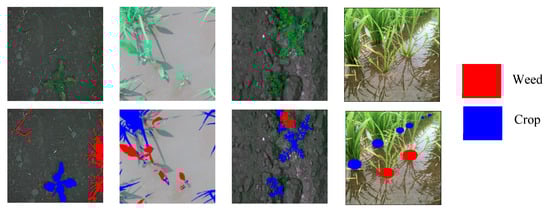
Figure 1. Crops and weeds segmentation datasets: BoniRob on left, followed by rice seeding weed, carrot weed, and paddy-millet: red color indicates weed and blue crop.

The proposed cascaded encoder-decoder (CED-Net), shown in Figure 2, consists of four small encoder-decoder networks divided into two levels. Encoder-decoder networks of each level, are trained independently either for crops segmentation or for weeds. More specifically, Model-1 and Model-2 are trained for weeds prediction while Model-3 and Model-4 are trained for the crops. The network was extended to two levels to extract features at different scales and to provide coarse-to-fine predictions. The contributions of this work can be summarized as: instead of building a big encoder-decoder network with millions of parameters, we can implement the same system with small networks in a cascaded form. The proposed architecture outperforms or is on par with U-Net [8], SegNet [9], FCN-8s [10], and DeepLabv3 [11] over intersection over union (IoU), F1-score, sensitivity, true detection rate (TDR), and average precision (AP) comparison metrics on rice seeding and weed, BoniRob, carrot crop vs. weed and a paddy-millet dataset. The proposed network has significantly fewer parameters, (1/5.74 × U-Net), (1/5.77 × SegNet), (1/3.04 × FCN-8s), and (1/3.24 × DeepLabv3) making it more efficient and applicable to embedded applications in agricultural robots. The pre-trained models, datasets information, and implementation details are available at https://github.com/kabbas570/CED-Net-Crops-and-Weeds-Segmentation.

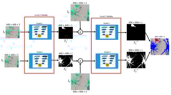
Figure 2. Architecture of the proposed cascaded encoder-decoder (CED-Net). All four models are trained independently. The target for Model-1 and Model-2 is weed while the target for Model-3 and Model-4 is the crop.

2. Related Work

In recent years, convolutional neural networks (CNNs) have been at the forefront of training algorithms, and are capable of both visualizing and identifying patterns in images with the minimum human intervention [12]. This capability has enabled the expansion of CNN’s applications to all fields of computer vision, including self-driving cars [13], facial recognition [14], stereo vision [15], medical image processing [16], agriculture [7], and bioinformatics [17].

In agriculture, CNNs have been used to solve a variety of problems. To differentiate between healthy and diseased plants, [18] proposed a deep learning-based model that is capable of identifying 26 different diseases in 14 crop species. The authors used pre-trained AlexNet [19] and GoogleNet [20] on a dataset of 54,306 images, to achieve a classification accuracy of greater than 99%. To estimate weed species and growth stages, [21] presented a method using pre-trained Inception-v3 architecture [22]. Their proposed model is capable of estimating the number of leaves with an accuracy of 70%.

To identify weed locations in leaf-occluded crops, [23] used DetectNet [24]. Their network was trained on 17,000 annotations of weeds images to identify weeds in cereal fields. The algorithm is 46% accurate in detecting weeds, however, it is unable to detect overlapping and small weeds. To specify herbicides for soybean crops, [25] proposed a CNN-based model to identify weeds and classify them either as grass or broadleaf. A sliding window-based approach was used in [3] for stem detection; each local window provides information about stem location or a non-stem region. Fuentes et al. developed an automated diagnosis system for tomato disease detection based on deep neural network, it also used long-short term memory (LSTM) to provide detailed descriptions of disease symptoms [23]. To obtain location information about weeds for site-specific weed management (SSWM), [5] introduced a dataset and performed experiments on a SegNet based encoder-decoder network (via transfer learning) for semantic segmentation that achieved a mean average accuracy as high as 92.7%.

Precise estimation of the stem location of crops or weeds, as well as the total area of coverage, is crucial to remove weeds either mechanically or by selective spraying. Lottes et al. introduced a network based on a single encoder and two separate decoders for plant and stem detection [3]. The authors also provided results that achieved by semantic segmentation in terms of the highest mean average precision of 87.3%. To increase the application of computer vision for agricultural benefits, [6] presented a dataset of 60 images for carrot crops and weeds detection. They also provided the semantic segmentation results in terms of different evaluation metrics like average accuracy, precision, recall, and F1-score.

Semantic segmentation based weeds and crops identification is the most challenging problem and needs to be solved for efficient smart farming, where the goal is to assign a separate class label to each pixel of the image [26]. The most popular deep supervised learning-based models for segmentation include FCN, SegNet, U-Net, DeepLabv3, ParseNet [27], PSPNet [28], MaskLab [29], TensorMask [30] and attention-based models include DANet [31], Chen et al. [32], OCNet [33] and, CCNet [34]. However, CNNs that used encoder (down-sampling)–decoder (up-sampling) structure (such as SegNet, U-Net, and) or a spatial pyramid pooling module (such as DeepLabv3) are considered as the most promising candidate for semantic segmentation tasks as they obtain sharp object boundaries or capture the contextual information at different resolution [35].

FCN is considered as a breaking point for segmentation literature, which is designed to make dense predictions without any fully connected layer [10]. FCN uses VGG-16 to extract the input image features. Different variants of FCN (FCN-8s, FCN-16s, and FCN-32s) are available and their attributes are different in terms of using the intermediate outputs. In contrast, SegNet is a symmetric encoder-decoder based segmentation network [9] where the encoder uses convolution and pooling operations to reduce the spatial dimensions of feature maps while storing the index of each extracted value from each window. The decoder of SegNet performs the up-sampling using stored max-pooling indices. Another symmetric encoder-decoder architecture is U-Net [8] where the features extraction of encoder is performed in four stages with two consecutive 3 × 3 convolutions followed by max-pooling and batch normalization. The bottleneck performs a sequence of two 3 × 3 convolutions and feedforward the feature maps to decoder where it up-samples the feature maps by 2 × 2 convolution and halves the number of feature maps before concatenating with the encoder. Afterwards, a sequence of two 3 × 3 convolutions are performed and the final segmentation map is generated with 1 × 1 convolutions. However, DeepLabv3 uses the concept of atrous convolution to adjust the filter’s field-of-view and atrous spatial pyramid pooling (ASPP) to consider objects at different scales [11].

The proposed CED-Net is designed to perform the semantic segmentation task on crops and weeds dataset and consists of cascaded encoder-decoder structure. Thus, for experiments and comparisons of evaluation matrices, we compared the proposed network with FCN-8s, SegNet, U-Net, and DeepLabv3.

3. Proposed Architecture

The proposed network architecture is shown in Figure 2. The overall model training is performed in two stages. At each level, two models are trained independently. At Level-1, Model-1 is trained for coarse weed prediction and Model-3 for crop prediction. The predictions of Model-1 and Model-3 are up-sampled, concatenated with corresponding input image size, and used as inputs by Model-2 and Model-4, respectively. Two cascaded networks (Model-1, Model-2) are thus trained for weed predictions, and the other two (Model-3, Model-4) for crop predictions. In total, then, we have four such small networks. The section that follows explains the network architecture and training details.

3.1. Spatial Sampling

A custom data generator function $f\left(I_1,I_2, T_1{}^{\prime },T_2{}^{\prime },T_1{}^{″},T_2{}^{″}\right)$ is defined for each encoder–decoder network to match input and output dimensions, and to prepare separate ground truths for crops and weeds. For Level-1, we used ($I_1, T_1{}^{\prime })$ and ($I_1, T_2{}^{\prime }),$ all images and their corresponding ground truths were resized to a spatial dimension of 448 × 448. Level-2 models were trained on ($I_2,T_1)$ and ($I_2,T_2)$ with spatial dimensions of 896 × 896. Bilinear interpolation was used in each case to adjust the spatial dimension of input images and targets as well as for up-sampling the Level-1 outputs for each encoder-decoder network to match dimensions with the next level. We started to train the networks with inputs of dimensions 448 × 448 for both weeds and crops as separate targets. At Level-1 two models were trained independently where for Model-1 the corresponding target was a binary mask of weeds and for Model-3 target was a binary mask of crops. If $M_i$ represents the model, then the output $u_i$ for input dimensions $I_{\frac{n}{2}\times \frac{n}{2}}$ can be defined as:

$$u_i=M_i\left(I_{\frac{n}{2}\times \frac{n}{2}}\right)$$

(1)

At Level-1, {i = 1, 3} and $u_i$ is the output of Level-1 and has the same dimension as input ($I_{\frac{n}{2}\times \frac{n}{2}}$), where n = 896. After training Level-1 models, their predictions were up-sampled, denoted by $U_i$, and concatenated with the input image ($I_{n\times n}$), which was further used as an input for Level-2 models. The output of Level-2 $v_{n\times n},$ has the dimensions of n × n and expressed as:

$$v_{n\times n} =M_i\left(U_{i-1},I_{n\times n}\right)$$

(2)

At Level-2, {i = 2, 4} and $U_{i-1}$ is the corresponding output of Level-1.

3.2. Encoder-Decoder Network

The detailed architecture of a single encoder-decoder network is shown in Figure 3. The input for this small network is an RGB image while the target is a binary mask with the same dimensions as the input. This network is similar to U-Net, but instead of going very deep, we limited the maximum number of feature maps to 256. For the encoder, the number of feature maps was increased as {16, 32, 64, and 128} while decreasing the spatial dimensions using 2 × 2 max-pooling [24] with stride = 2 that results in feature maps subsampling by a factor of 2. In the bottleneck, the maximum number of feature maps was set to 256. For the decoder, the bottleneck feature maps were decreased as {128, 64, 32, and 16} while increasing their spatial dimensions by a factor of 2 through bilinear interpolation. At each stage of the decoder, the up-sampled feature maps were concatenated with corresponding feature maps of the encoder, indicated by a horizontal arrow shown in Figure 3.

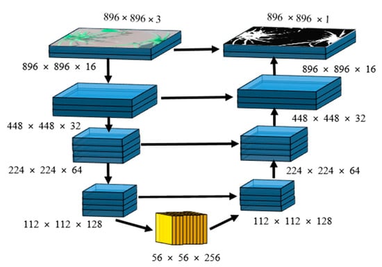
Figure 3. A single encoder-decoder network, which is used in the cascaded form in Figure 2.

A rectified linear unit (ReLU) was used as an activation function for each convolutional layer of encoder, bottleneck, and decoder, whereas for the output layer used sigmoid. Model-1 and Model-3 encoder–decoder networks have 1,352,881 parameters whereas Model-2 and Model-4 have 1,353,025 parameters. This increment in the number of parameters happens because the input dimensions for Level-2 (Model-2, Model-4) are 896 × 896 × 4 rather than 896 × 896 × 3 of Level-1 (Model-1, Model-3). The concatenation of up-sampled predictions of Level-1 with input images increases the input channel of Level-2 by 1. In total, the proposed architecture comprises 5,411,812 parameters.

3.3. Post-Processing

As a post-processing step, the outputs of Level-2 are combined by concatenating their predictions, as shown in Figure 2 and the final output is then mapped onto the input images. To differentiate between crops and weeds, we assigned red color to weeds and blue color to crops for all four datasets. Background pixels were kept the same as in the original input image.

3.4. Network Training

For each target (i.e., either weed or crop), network training was performed in two stages. In the first phase, Level-1 models (Model-1 and Model-3) were trained independently to produce coarse outputs. Level-2 models (Model-2 and Model-4) were trained in the second phase by utilizing the predictions from Level-1 models as initialization in a concatenated form with the input image.

All four models were trained using Adam optimization [25], with β₁ = 0.9 and β₂ = 0.99, learning rate = 0.0001 with a batch size = 2. A custom loss function was defined in terms of dice coefficient [26],

$$\mathrm{Loss}=1-\left[\frac{2\times \left(Target\cap Prediction\right)}{\left(Target+Prediction\right)}\right]$$

(3)

4. Evaluation Metrics

To measure and compare the quantitative performance of the proposed network, different evaluation measures such as dice coefficient/F1-score, Jaccard similarity (JS)/intersection over Union (IoU), sensitivity/recall, true detection rate (TDR), and average precision (AP) were measured. These metrics were computed by identifying the variables true positive (TP), true negative (TN), false positive (FP), and false-negative (FN) by calculating the confusion matrix between the prediction and the ground truth. The expressions for IoU, recall, TDR, and precision are defined as:

$$IoU=\frac{TP}{\left(TP+FN+FP\right)}$$

(4)

$$Recall=\frac{TP}{\left(TP+FN\right)}$$

(5)

$$TDR=1-\frac{FN}{\left(TP+FN\right)}$$

(6)

$$Precision=\frac{TP}{\left(TP+FP\right)}$$

(7)

F1-score is computed from the harmonic mean of precision and recall and expressed as:

$$F1\_Score=\frac{\left(2\times Precision\times Recall\right)}{\left(Precision+Recall\right)}$$

(8)

The average precision is calculated for the paddy-millet dataset using 11-points interpolation [27], the maximum precision values ($P_{interp}\left(R\right)$) are found at a set of 11 equally spaced recall values [0, 0.1, 0.2, ... 1] and by averaging them we calculated the $A{P}_{11}$, as given by:

$$A{P}_{11}=\frac{1}{11}{\displaystyle \sum }_{R\in \left\{0,0.1,0.2\dots 0.9,1\right\}}{P}_{interp}\left(R\right)$$

(9)

where

$$P_{interp}\left(R\right)={}_{\tilde{R}:\tilde{R}>R}^{\hspace{1em} max}P\left(\tilde{R}\right)$$

(10)

Therefore, the average precision is obtained by considering only the maximum precision values $P_{interp}\left(R\right)$ whose recall values are greater than R. The mean average precision (mAP) is simply the average of AP over all classes (rice and millet) and expressed as:

$$mAP=\frac{1}{N}{\displaystyle \sum }_{i=1}^{N}A{P}_i$$

(11)

5. Datasets

To evaluate and compare the proposed model, we used four different publicly-available datasets that are related to the identification of crops and weeds for smart farming. For each dataset, the goal is to perform a pixel-wise prediction of crops and weeds. Table 1 summarizes the details of each dataset and distribution of data for training, validation, and testing.

Table 1. Dataset distribution for training, validation, and testing.

Dataset	Total Images	Training	Validation	Testing
Rice seeding and weed	224	160	20	44
BoniRob	492	400	30	62
Carrot crop vs. weed	60	45	5	10
Paddy-millet	380	310	30	40

5.1. Rice Seeding and Weed Segmentation Dataset

This dataset is provided by [5] and contains a total of 224 images of size 912 × 1024 which were captured using a Canon IXUS 1000 HS (EF-S 36–360 mm f/3.4–5.6 IS STM) camera. Each image came with a corresponding ground truth-annotated label with two classes: rice and Sagittaria trifolia weed, which is quite harmful to rice crops [28]. Among 224 total images, 160 images were used for training, 20 for validation, and 44 for testing. The dataset is publicly available at: https://figshare.com/articles/rice_seedlings_and_weeds/7488830.

5.2. BoniRob Dataset

An autonomous robot, named BoniRob [4] was used to collect this dataset in 2016 from fields near Bonn, Germany. The BoniRob dataset contains sugar beet plants, dicot weeds, and grass weeds. For the experiments, we used a subset of the BoniRob dataset containing sugar beets and grass weeds; 492 images of size 1296 × 966 were used, divided into training (400), validation (30), and holdout test (62). This dataset is publicly available at: http://www.ipb.uni-bonn.de/data/sugarbeets2016/.

5.3. Carrot Crop and Weed

The carrot crop and weed dataset contains a total of 60 images of the size 1296 × 966 and was introduced by [6]. Images were captured using the JAI AD-130GE camera model from organic carrot fields in a region of northern Germany. Annotation of ground-truth labels of weeds and crops were conducted manually. Among 60 images 45, 5, and 10 were used as training, validation, and testing respectively. The dataset can be found at: https://github.com/cwfid.

5.4. Paddy-Millet Dataset

The paddy-millet dataset is acquired from [7] and contains a total of 380 images of size 804 × 604 which are captured using a handheld Canon camera EOS-200D. The paddy and millet weeds have a similar appearance so it’s a very challenging dataset and the goal is to identify and localize the paddy and weed location using semantic graphics. The semantic graphics is the idea of labeling an area of interest with minimum human labor. In our experiments, we have manually assigned a solid circle to the base of paddy and millet weed and the rest of the pixels are counted as background. We have used 380 images of this dataset and are distributed as 310 for training, 30 for validation, and 40 for testing.

6. Experimental Results and Discussion

All experiments mentioned in this paper were performed using a PC equipped with an NVIDIA Titan XP GPU. We used the Keras framework with a Tensorflow backend. Both quantitative and qualitative results of CED-Net and other state-of-the-art networks were compared for all datasets. Table 2 shows the number of parameters for the different architecture used in this paper. Observe that the proposed architecture has a smaller number of parameters compared to others: almost 6 times less than U-Net and SegNet, and 3 times fewer parameters than FCN-8s and DeepLabv3.

Table 2. Total number of parameters for different architectures (bold number represents the best results in the table).

Architecture	Total Params (in million)
U-Net	31.04
SegNet	31.24
FCN-8s	16.49
DeepLabv3	17.56
Proposed (CED-Net)	5.41

6.1. Rice Seeding and Weed Segmentation

For quantitative analysis, between the proposed CED-Net and other networks on rice seeding and weed dataset, we computed different metrics such as intersection over union (IoU) individually for each class (i.e., weed IoU and crop IoU) and mean intersection over union (mIoU) for both classes together, F1-score and sensitivity. For every evaluation index, our proposed CED-Net outperforms other networks with distinctive margins. Table 3 summarizes the segmentation performance of our proposed architecture against each evaluation metric and all other networks.

Table 3. Comparison of evaluation metrics for rice seeding and weed dataset (bold number represents the best results in the table).

Architecture	Crop IoU	Weed IoU	mIoU	F1-Score	Sensitivity
U-Net	0.5879	0.6267	0.5967	0.7474	0.6370
SegNet	0.6736	0.6760	0.6741	0.8053	0.7613
FCN-8s	0.5430	0.5652	0.5478	0.7078	0.5640
DeepLabv3	0.6796	0.6638	0.6760	0.8067	0.7513
CED-Net (proposed)	0.7088	0.7170	0.7105	0.8308	0.7995

The experimental results of all the networks for the rice seeding and weed dataset are shown in Figure 4. The column on the far left shows input images for each network; the result is shown on the input image, with red indicating the Sagittaria trifolia weed and blue the rice crop. The proposed network performed well in differentiating between weeds and crops, whereas the other architectures were at times unsuccessful in assigning the label to pixels, which explains their higher FN rates (SegNet, 3.13%; U-Net, 4.76%; FCN-8s, 5.72%, and DeepLabv3, 3.2%) compared to the proposed network (2.63%), as mentioned in Table 4.

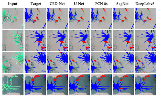
Figure 4. Qualitative comparison of results of semantic segmentation for rice seeding and weed dataset.

Table 4. Confusion matrices of SegNet, U-Net, FCN-8s, DeepLabv3, and proposed CED-Net for rice seeding and weed dataset.

SegNet				U-Net
n = 70,647,808	Predicted: YES	Predicted: NO		n = 70,647,808	Predicted: YES	Predicted: NO
Actual: YES	TP = 7,060,518	FN = 2,213,496		Actual: YES	TP = 5,908,166	FN = 3,365,848
Actual: NO	FP = 1,199,162	TN = 60,174,632		Actual: NO	FP = 626,197	TN = 60,747,597
		Proposed CED-Net
		n = 70,647,808	Predicted: YES	Predicted: NO
		Actual: YES	TP = 7,414,952	FN = 1,859,062
		Actual: NO	FP = 1,160,842	TN = 60,212,952
FCN-8s				DeepLabv3
n = 70,647,808	Predicted: YES	Predicted: NO		n = 70,647,808	Predicted: YES	Predicted: NO
Actual: YES	TP = 5,231,318	FN = 4,042,696		Actual: YES	TP = 6,967,874	FN = 2,306,14
Actual: NO	FP = 274,874	TN = 61,098,920		Actual: NO	FP = 1,032,689	TN = 60,341,105

6.2. BoniRob Dataset Segmentation

For this dataset, 62 images were used as testing samples, and comparative quantitative analysis was performed as shown in Table 5. Proposed CED-Net outperforms U-Net, SegNet, FCN-8s, and DeepLabv3 for crop IoU, mIoU, and F1-score metric. However, U-Net performs marginally better over weed IoU and sensitivity metrics with 6 times higher parameters than the CED-Net.

Table 5. Experimental results of the proposed approach for BoniRob dataset as opposed to other architectures (bold number represents the best results in the table).

Architecture	Crop IoU	Weed IoU	mIoU	F1-Score	Sensitivity
U-Net	0.9023	0.7266	0.8274	0.9055	0.9129
SegNet	0.8417	0.6175	0.7411	0.8513	0.8248
FCN-8s	0.8743	0.5022	0.7245	0.8402	0. 7337
DeepLabv3	0.9230	0.6834	0.8257	0.9045	0.8665
CED-Net (proposed)	0.9179	0.7149	0.8344	0.9097	0.8968

It can be seen from the SegNet column that it often misclassifies the crop label with weed whereas the better performance is obtained from CED-Net. The confusion matrices from Table 6, show that the proposed CED-Net has ~1.7 times, ~2.5 times, and ~1.3 times less false negatives (FN) than SegNet, FCN-8s, and DeepLabv3 respectively, and marginally higher than U-Net. The qualitative results of the BoniRob dataset for all the networks are shown in Figure 5.

Table 6. Confusion matrices of SegNet, U-Net, FCN-8s, DeepLabv3, and proposed CED-Net for BoniRob dataset.

SegNet				U-Net
n = 99,549,184	Predicted: YES	Predicted: NO		n = 99,549,184	Predicted: YES	Predicted: NO
Actual: YES	TP = 3,796,991	FN = 806,115		Actual: YES	TP = 4,202,492	FN = 400,614
Actual: NO	FP = 520,048	TN = 94,426,030		Actual: NO	FP = 475,841	TN = 94,470,237
		Proposed CED-Net
		n = 99,549,184	Predicted: YES	Predicted: NO
		Actual: YES	TP = 4,128,345	FN = 474,761
		Actual: NO	FP = 344,371	TN = 94,601,707
FCN-8s				DeepLabv3
n = 99,549,184	Predicted: YES	Predicted: NO		n = 99,549,184	Predicted: YES	Predicted: NO
Actual: YES	TP = 3,377,705	FN = 1,225,401		Actual: YES	TP = 39,88,677	FN = 614,429
Actual: NO	FP = 58,716	TN = 94,887,362		Actual: NO	FP = 227,169	TN = 94,718,909

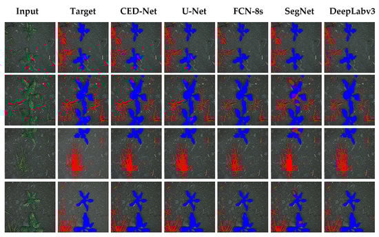
Figure 5. Semantic segmentation results for BoniRob dataset.

6.3. Carrot Crop and Weed Segmentation

The carrot crop and weed dataset is a small dataset, containing only 60 out of which 10 were used as a test set. The evaluation metrics of proposed CED-Net and other comparing architectures are listed in Table 7. Except for the sensitivity metric, the CED-Net outperforms all other comparing networks with huge margins. However, CED-Net marginally underperforms than SegNet over sensitivity metric as SegNet generates the highest number of TP’s (2.6% compared to CED-Net 2.5%), a lower number of FN’s (0.33% as compared to CED-Net 0.48%) but SegNet produces 8 times more FP’s than CED-Net which reduces its overall performance as shown in Table 8. In the U-Net case, it generates the lowest number of FP’s (19,138) but its performance is penalized by a higher number of FNs (111,531).

Table 7. Evolution of proposed architecture compared with other networks (bold number represents the best results in the table).

Architecture	Crop IoU	Weed IoU	mIoU	F1-Score	Sensitivity
U-Net	0.7775	0.6661	0.7406	0.8510	0.7699
SegNet	0.5276	0.5717	0.5394	0.7008	0.8877
FCN-8s	0.6208	0.5411	0.5931	0.7446	0.6695
DeepLabv3	0.7550	0.6144	0.7074	0.8286	0.7581
CED-Net (proposed)	0.8120	0.7016	0.7761	0.8739	0.8385

Table 8. Confusion matrices of SegNet, U-Net, FCN-8s, DeepLabv3, and proposed CED-Net for carrot crop and weed dataset.

SegNet				U-Net
n = 16,056,320	Predicted: YES	Predicted: NO		n = 16,056,320	Predicted: YES	Predicted: NO
Actual: YES	TP = 430,309	FN = 54,434		Actual: YES	TP = 373,212	FN = 111,531
Actual: NO	FP = 312,887	TN = 15,258,690		Actual: NO	FP = 19,138	TN = 15,552,439
		Proposed CED-Net
		n = 16,056,320	Predicted: YES	Predicted: NO
		Actual: YES	TP = 406,497	FN = 78,246
		Actual: NO	FP = 39,020	TN = 15,532,557
FCN-8s				DeepLabv3
n = 16,056,320	Predicted: YES	Predicted: NO		n = 16,056,320	Predicted: YES	Predicted: NO
Actual: YES	TP = 324,555	FN = 160,188		Actual: YES	TP = 367,505	FN = 117,238
Actual: NO	FP = 62,454	TN = 15,509,123		Actual: NO	FP = 34,715	TN = 15,536,862

The proposed CED-Net performed better than any other network for most evaluation indices and can compete with other networks by predicting the minimum number of FPs and FNs while increasing the number of TPs and TNs. Figure 6 illustrates a qualitative comparison for all the networks. The proposed network performed well in classifying weed pixels, although in some cases it was unable to assign a label to crop pixels; thus, its IoU is lower for crops than for weeds. The SegNet column shows that it was unable to differentiate boundaries well, indicated by its high FP rate.

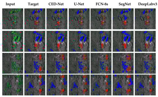
Figure 6. Qualitative analysis for carrot crop and weed dataset.

6.4. Paddy-Millet Dataset

The quantitative performance for this dataset is measured using AP for weed and rice, mAP, and TDR. In the paddy-millet dataset, stamping-out is one of the most effective and environment-friendly techniques to remove the millet weed from rice crops. For the stamping-out technique, finding the class (i.e., millet or weed) and location of the weeds is more important than finding the area covered by them. Since the coordinates of the location of millet weeds and paddy have higher significance, hence it is more useful to find the center point of the detections. Thus, for this dataset, we used TDR, AP, and mAP as evaluation metrics to analyze the performance of the network.

A prediction provided by the network is to be classified as TP, FN, or FP where the category is classified using the Euclidian distance between the centers of prediction and ground truth. If the Euclidian distance between the centers of prediction and ground truth is less than a pre-defined threshold it is counted as TP. However, if the distance is greater than the threshold, two penalties are imposed on the network: (1) detection at the wrong location (FP) and (2) missing of the ground truth (FN). True detection rate (TDR) values are computed using Equation (6) which determines the performance of the network to identify crops (paddy) and the weeds (millet) locations within the defined threshold. Table 9 shows the TDR values of the proposed CED-Net along with comparing networks and illustrates that the proposed network outperforms all other networks with significantly fewer parameters.

Table 9. Results using true detection rate (TDR) variants, the number next to the TDR represents different threshold levels (bold number represents the best results in the table).

Approach	TDR: 10	TDR: 15	TDR: 20
U-Net	0.3716	0.5468	0.6193
SegNet	0.3957	0.5649	0.6767
FCN-8s	0.4018	0.5981	0.6888
DeepLabv3	0.3806	0.6223	0.7401
CED-Net	0.4531	0.6314	0.6918

For further evaluation, we also provided the results in terms of AP for weeds, AP for paddy, and mAP. Precision is defined as the capability of a model to locate relevant objects only and recall is true positive detections relative to all ground truths. The 11-points interpolation is used to find AP (see Equation (9)) for each class (i.e., rice crops and millet weeds) separately and mAP is computed (from Equation (10)) with N = 2 (number of classes). Table 10 illustrates the AP for weed, rice, and mAP results. The proposed CED-Net has the highest mAP for all threshold and can detect most of the millet weeds and rice crops as compared to the other networks as listed in Table 10. The qualitative results for the paddy-millet dataset are presented in Figure 7.

Table 10. Results using average precision (AP) and mean average precision (mAP) variants, the number next to the AP/mAP represents different threshold levels (bold number represents the best results in the table).

Approach	mAP:10		mAP:15		mAP:20
	Rice AP:10	Weed AP:10	Rice AP:15	Weed AP:15	RiceAP:20	Weed AP:20
U-Net	0.13916		0.37254		0.4490
	0.14150	0.1368	0.3449	0.4001	0.4492	0.4487
SegNet	0.2302		0.4278		0.5576
	0.2109	0.2494	0.3864	0.4692	0.5255	0.5897
FCN-8s	0.2187		0.4280		0.5418
	0.1505	0.2870	0.4225	0.4336	0.5591	0.5245
Deeplabv3	0.1405		0.3796		0.5276
	0.1552	0.1257	0.4389	0.3204	0.6041	0.4512
CED-Net	0.3023		0.4913		0.5570
	0.3698	0.2367	0.5175	0.4651	0.6228	0.4913

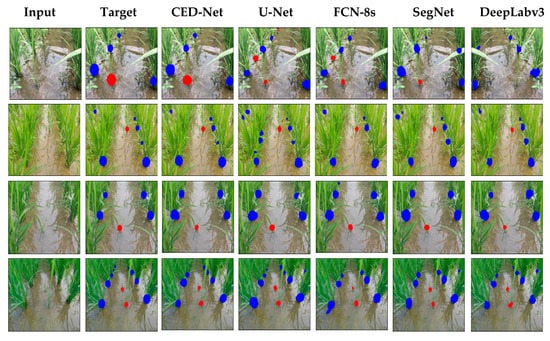
Figure 7. Experimental results of the paddy-millet dataset.

7. Conclusions

This paper presents a small-cascaded encoder-decoder (CED-Net) architecture to detect and extract the precise location of weeds and crops on farmland using semantic segmentation. The proposed network has comparatively less number of parameters compared to the other state-of-the-art architectures, thus results in lesser training and inference time. The improved performance of CED-Net is attributed to its coarse-to-fine approach and cascaded architecture. The network architecture is extended to two levels, at each of which two small encoder-decoder networks are trained independently in parallel, (i.e., one for crop predictions and the other for weed). At each level, the network aims either to predict a binary mask for crops or weeds. The predictions of Level-1, are further refined by Level-2 encoder-decoder networks to generate the final output. Thus, four small networks were trained, with two arranged in cascaded for each target (i.e., crops and weeds). To evaluate and compare the performance of the proposed CED-Net with other networks, we used four different publicly-available crops and weeds datasets. The proposed network has 1/5.74, 1/5.77, 1/3.04, and 1/3.24 times fewer parameters than U-Net, SegNet, FCN-8s, and DeepLabv3 respectively, which makes it more robust and hardware friendly compare to the other networks. Moreover, CED-Net either outperforms or is on par with other state-of-the-art networks in terms of different evaluation metrics such as mIoU, F1-score, sensitivity, TDR, and mAP.

References

- Fennimore, S.A.; Slaughter, D.C.; Siemens, M.C.; Leon, R.G.; Saber, M.N. Technology for Automation of Weed Control in Specialty Crops. Weed Technol. 2016, 30, 823–837. [Google Scholar] [CrossRef]
- Shaner, D.L.; Beckie, H.J. The future for weed control and technology. Pest Manag. Sci. 2014, 70, 1329–1339. [Google Scholar] [CrossRef] [PubMed]
- Lottes, P.; Behley, J.; Chebrolu, N.; Milioto, A.; Stachniss, C. Joint Stem Detection and Crop-Weed Classification for Plant-Specific Treatment in Precision Farming. In Proceedings of the 2018 IEEE/RSJ International Conference on Intelligent Robots and Systems (IROS), Madrid, Spain, 1–5 October 2018. [Google Scholar]
- Chebrolu, N.; Lottes, P.; Schaefer, A.; Winterhalter, W.; Burgard, W.; Stachniss, C. Agricultural robot dataset for plant classification, localization and mapping on sugar beet fields. Int. J. Robot. Res. 2017, 36, 1045–1052. [Google Scholar] [CrossRef]
- Ma, X.; Deng, X.; Qi, L.; Jiang, Y.; Li, H.; Wang, Y.; Xing, X. Fully convolutional network for rice seedling and weed image segmentation at the seedling stage in paddy fields. PLoS ONE 2019, 14, e0215676. [Google Scholar] [CrossRef] [PubMed]
- Haug, S.; Ostermann, J. A Crop/Weed Field Image Dataset for the Evaluation of Computer Vision Based Precision Agriculture Tasks. In European Conference on Computer Vision; Springer: Berlin/Heidelberg, Germany, 2014. [Google Scholar]
- Adhikari, S.P.; Yang, H.; Kim, H. Learning Semantic Graphics Using Convolutional Encoder–Decoder Network for Autonomous Weeding in Paddy Field. Front. Plant Sci. 2019, 10, 1404. [Google Scholar] [CrossRef] [PubMed]
- Ronneberger, O.; Fischer, P.; Brox, T. U-net: Convolutional networks for biomedical image segmentation. In International Conference on Medical Image Computing and Computer-Assisted Intervention; Springer: Berlin/Heidelberg, Germany, 2015. [Google Scholar]
- Badrinarayanan, V.; Badrinarayanan, V.; Cipolla, R. SegNet: A Deep Convolutional Encoder-Decoder Architecture for Image Segmentation. IEEE Trans. Pattern Anal. Mach. Intell. 2017, 39, 2481–2495. [Google Scholar] [CrossRef] [PubMed]
- Long, J.; Shelhamer, E.; Darrell, T. Fully convolutional networks for semantic segmentation. In Proceedings of the IEEE Conference on Computer Vision and Pattern Recognition, Boston, MA, USA, 7–12 June 2015. [Google Scholar]
- Chen, L.-C.; Papandreou, G.; Schroff, F.; Adam, H. Rethinking Atrous Convolution for Semantic Image Segmentation. arXiv 2017, arXiv:1706.05587. [Google Scholar]
- Pouyanfar, S.; Sadiq, S.; Yan, Y.; Tian, H.; Tao, Y.; Reyes, M.P.; Shyu, M.; Chen, S.; Iyengar, S.S. A survey on deep learning: Algorithms, techniques, and applications. ACM Comput. Surv. 2018, 51, 1–36. [Google Scholar] [CrossRef]
- Bojarski, M.; Del Testa, D.; Dworakowski, D.; Firner, B.; Flepp, B.; Goyal, P.; Jackel, L.D.; Monfort, M.; Müller, U.; Zhang, J.; et al. End to End Learning for Self-Driving Cars. arXiv 2016, arXiv:1604.07316. [Google Scholar]
- Schroff, F.; Kalenichenko, D.; Philbin, J. FaceNet: A unified embedding for face recognition and clustering. In Proceedings of the 2015 IEEE Conference on Computer Vision and Pattern Recognition (CVPR), Boston, MA, USA, 7–12 June 2015. [Google Scholar]
- Smolyanskiy, N.; Kamenev, A.; Birchfield, S. On the Importance of Stereo for Accurate Depth Estimation: An Efficient Semi-Supervised Deep Neural Network Approach. In Proceedings of the 2018 IEEE/CVF Conference on Computer Vision and Pattern Recognition Workshops (CVPRW), Salt Lake City, UT, USA, 18–22 June 2018. [Google Scholar]
- Abbas, Z.; Rehman, M.-U.; Najam, S.; Rizvi, S.D. An Efficient Gray-Level Co-Occurrence Matrix (GLCM) based Approach towards Classification of Skin Lesion. In Proceedings of the 2019 Amity International Conference on Artificial Intelligence (AICAI), Amity University, Dubai, UAE, 4–6 February 2019. [Google Scholar]
- Mahmoudi, O.; Wahab, A.; Chong, K.T. iMethyl-Deep: N6 Methyladenosine Identification of Yeast Genome with Automatic Feature Extraction Technique by Using Deep Learning Algorithm. Genes 2020, 11, 529. [Google Scholar] [CrossRef] [PubMed]
- Mohanty, S.P.; Hughes, D.P.; Salathé, M. Using Deep Learning for Image-Based Plant Disease Detection. Front. Plant Sci. 2016, 7, 1419. [Google Scholar] [CrossRef] [PubMed]
- Krizhevsky, A.; Sutskever, I.; Hinton, G.E. ImageNet classification with deep convolutional neural networks. In Proceedings of the Advances in Neural Information Processing Systems (NIPS), Lake Tahoe, NV, USA, 3–6 December 2012. [Google Scholar]
- Szegedy, C.; Liu, W.; Jia, Y.; Sermanet, P.; Reed, S.; Anguelov, D.; Erhan, D.; Vanhoucke, V.; Rabinovich, A. Going deeper with convolutions. In Proceedings of the 2015 IEEE Conference on Computer Vision and Pattern Recognition (CVPR), Boston, MA, USA, 7–12 June 2015; Volume 18, pp. 1–9. [Google Scholar]
- Teimouri, N.; Dyrmann, M.; Nielsen, P.R.; Mathiassen, S.; Somerville, G.; Jørgensen, R.N. Weed Growth Stage Estimator Using Deep Convolutional Neural Networks. Sensors 2018, 18, 1580. [Google Scholar] [CrossRef] [PubMed]
- Szegedy, C.; Vanhoucke, V.; Ioffe, S.; Shlens, J.; Wojna, Z. Rethinking the Inception Architecture for Computer Vision. In Proceedings of the 2016 IEEE Conference on Computer Vision and Pattern Recognition (CVPR), Las Vegas, NV, USA, 26 June–1 July 2016. [Google Scholar]
- Dyrmann, M.; Jørgensen, R.N.; Midtiby, H.S. RoboWeedSupport—Detection of weed locations in leaf occluded cereal crops using a fully convolutional neural network. Adv. Anim. Biosci. 2017, 8, 842–847. [Google Scholar] [CrossRef]
- Barker, J.; Sarathy, S.; Tao, A. DetectNet: Deep Neural Network for Object Detection in DIGITS. Nvidia, 2016. Available online: https://devblogs.nvidia.com/parallelforall/detectnet-deep-neural-network-object-detection-digits/ (accessed on 30 November 2016).
- Ferreira, A.D.S.; Freitas, D.M.; Da Silva, G.G.; Pistori, H.; Folhes, M.T. Weed detection in soybean crops using ConvNets. Comput. Electron. Agric. 2017, 143, 314–324. [Google Scholar] [CrossRef]
- Minaee, S.; Boykov, Y.; Porikli, F.; Plaza, A.; Kehtarnavaz, N.; Terzopoulos, D. Image Segmentation Using Deep Learning: A Survey. arXiv 2015, arXiv:1506.04579. [Google Scholar]
- Liu, W.; Rabinovich, A.; Berg, A.C. Parsenet: Looking Wider to See Better. arXiv 2015, arXiv:1506.04579. [Google Scholar]
- Zhao, H.; Shi, J.; Qi, X.; Wang, X.; Jia, J. Pyramid Scene Parsing Network. In Proceedings of the 2017 IEEE Conference on Computer Vision and Pattern Recognition (CVPR), Honolulu, HI, USA, 21–26 July 2017. [Google Scholar]
- Chen, L.-C.; Hermans, A.; Papandreou, G.; Schroff, F.; Wang, P.; Adam, H. MaskLab: Instance Segmentation by Refining Object Detection with Semantic and Direction Features. In Proceedings of the 2018 IEEE/CVF Conference on Computer Vision and Pattern Recognition, Salt Lake City, UT, USA, 18–23 June 2018. [Google Scholar]
- Chen, X.; Girshick, R.; He, K.; Dollar, P. TensorMask: A Foundation for Dense Object Segmentation. In Proceedings of the 2019 IEEE/CVF International Conference on Computer Vision (ICCV), Seoul, Korea, 27–28 October 2019. [Google Scholar]
- Fu, J.; Liu, J.; Tian, H.; Li, Y.; Bao, Y.; Fang, Z.; Lu, H. Dual Attention Network for Scene Segmentation. In Proceedings of the 2019 IEEE/CVF Conference on Computer Vision and Pattern Recognition (CVPR), Long Beach, CA, USA, 15–20 June 2019. [Google Scholar]
- Chen, L.-C.; Yang, Y.; Wang, J.; Xu, W.; Yuille, A.L. Attention to Scale: Scale-Aware Semantic Image Segmentation. In Proceedings of the 2016 IEEE Conference on Computer Vision and Pattern Recognition (CVPR), Las Vegas, NV, USA, 26 June–1 July 2016. [Google Scholar]
- Yuan, Y.; Wang, J. Ocnet: Object Context Network for Scene Parsing. arXiv 2018, arXiv:1809.00916. [Google Scholar]
- Huang, Z.; Huang, L.; Gong, Y.; Huang, C.; Wang, X. Mask Scoring R-CNN. In Proceedings of the 2019 IEEE/CVF Conference on Computer Vision and Pattern Recognition (CVPR), Long Beach, CA, USA, 15–20 June 2019. [Google Scholar]
- Chen, L.-C.; Zhu, Y.; Papandreou, G.; Schroff, F.; Adam, H. Encoder-Decoder with Atrous Separable Convolution for Semantic Image Segmentation. In Proceedings of the European Conference on Computer Vision (ECCV), Munich, Germany, 8–14 September 2018. [Google Scholar]
© 2020 by the authors. Licensee MDPI, Basel, Switzerland. This article is an open access article distributed under the terms and conditions of the Creative Commons Attribution (CC BY) license (http://creativecommons.org/licenses/by/4.0/).