Article

Non-Uniform Discretization-based Ordinal Regression for Monocular Depth Estimation of an Indoor Drone

1
Key Laboratory of Autonomous Systems and Networked Control, Ministry of Education, Unmanned Aerial Vehicle Systems Engineering Technology Research Center of Guangdong, South China University of Technology, Guangzhou 510640, China
2
School of Computer Science and Technology, Guangdong University of Technology, Guangzhou 510006, China
3
UTA Research Institute, University of Texas at Arlington, Fort Worth, TX 76019, USA
*
Author to whom correspondence should be addressed.
Electronics 2020, 9(11), 1767; https://doi.org/10.3390/electronics9111767
Submission received: 25 September 2020 / Revised: 18 October 2020 / Accepted: 21 October 2020 / Published: 23 October 2020
(This article belongs to the Section Systems & Control Engineering)

Abstract

:
At present, the main methods of solving the monocular depth estimation for indoor drones are the simultaneous localization and mapping (SLAM) algorithm and the deep learning algorithm. SLAM requires the construction of a depth map of the unknown environment, which is slow to calculate and generally requires expensive sensors, whereas current deep learning algorithms are mostly based on binary classification or regression. The output of the binary classification model gives the decision algorithm relatively rough control over the unmanned aerial vehicle. The regression model solves the problem of the binary classification, but it carries out the same processing for long and short distances, resulting in a decline in short-range prediction performance. In order to solve the above problems, according to the characteristics of the strong order correlation of the distance value, we propose a non-uniform spacing-increasing discretization-based ordinal regression algorithm (NSIDORA) to solve the monocular depth estimation for indoor drone tasks. According to the security requirements of this task, the distance label of the data set is discretized into three major areas—the dangerous area, decision area, and safety area—and the decision area is discretized based on spacing-increasing discretization. Considering the inconsistency of ordinal regression, a new distance decoder is produced. Experimental evaluation shows that the root-mean-square error (RMSE) of NSIDORA in the decision area is 33.5% lower than that of non-uniform discretization (NUD)-based ordinal regression methods. Although it is higher overall than that of the state-of-the-art two-stream regression algorithm, the RMSE of the NSIDORA in the top 10 categories of the decision area is 21.8% lower than that of the two-stream regression algorithm. The inference speed of NSIDORA is 3.4 times faster than that of two-stream ordinal regression. Furthermore, the effectiveness of the decoder has been proved through ablation experiments.

1. Introduction

In the past decade, drones have greatly promoted the rapid development of aviation [1], and have been widely used in different fields such as search and rescue [2], infrastructure inspection [3], speed measurement of a moving vehicle [4], and so on. At the same time, recent research has mainly focused on enhancing the autonomy of drones through deep learning algorithms [5,6] because deep learning has achieved advanced performance in visual tasks.
In order to solve the problem of autonomous navigation by indoor drones, the traditional approach is to use the simultaneous localization and mapping (SLAM) algorithm [7,8,9] based on expensive sensors such as device obtaining ordinary RGB three-channel color + depth map (RGB-D) [7], LIDAR [10], etc. The dense structure from motion (SFM) algorithm [11,12] relies on a single moving camera [13] to construct a three-dimensional map of the environment, then the custom path planning algorithm takes the depth map as its input and outputs control signals to control the aircraft’s navigation. However, cheap commercial drones are usually equipped with a single camera, and the SLAM method usually requires heavyweight expensive sensors, which limits the application of this method to commercial drones; in addition, this method requires expensive calculation costs when rebuilding the map, which greatly reduces the ability of real-time processing of images. The SFM-based obstacle avoidance method obtains a control signal to control a drone by means of the hover-map-plan-path-moving-hover method. This method cannot avoid dynamic obstacles when moving during or between mapping periods. When these algorithms are running in a real indoor dynamic environment, unrecoverable errors will occur for surfaces with less texture, such as white walls [14].
As a result that commercial drones are usually equipped with a forward-looking camera and do not require extra sensors [15], depth estimation based on monocular vision has aroused great interest. At the same time, recent studies have mainly used the deep learning (DL) algorithm to extract features to enhance the autonomy of drones [5], because the features extracted by this algorithm show better performance than manual feature extraction [13], and this method makes the end-to-end learning method possible [13].
In this direction, some researchers have used demonstration learning [16,17] or reinforcement learning [18,19] to process the original monocular image output control commands, and have achieved impressive results in autonomous navigation of the drone [16,17,18,19]. In the former method, the imitation learning strategy is used to label human actions as autonomous navigation. However, the data collected in this way are biased because humans will control the drone to avoid hitting obstacles. This means that demonstrative learning cannot be extended to a trajectory beyond a training demonstration of the human controller, which limits our ability to generalize the model. The latter method generates rewards or penalties for unseen environments through constant interaction between the drone and the environment—that is, the algorithm has a trial-and-error nature. As a result, the algorithm may make irreparable wrong decisions, which poses a serious threat to the safety of drones and the environment. Although Sadeghi et al. [19] achieved good unmanned aerial vehicle (UAV) navigation results through data simulation and reinforcement learning methods, the gap between the simulation environment and the real environment limits the application and promotion of reinforcement learning in reality [20].
In previous studies, the task of depth estimation for indoor drones have been considered either as classification problems [21,22] or as regression problems [14]. This article is the first to propose a deep learning method based on ordinal regression to solve this task. The main contributions of this work are summarized as follows:
  • We propose a non-uniform spacing-increasing discretization (NSID) strategy to discretize the distance labels of the data set, obtained by self-supervising. Three areas—a dangerous area, a decision area, and a safe area—are discretized by the NSID strategy. The evaluation of the strategy is shown in Section 4.2.
  • The monocular depth estimation of indoor drone problems is converted into an ordinal regression problem. Images obtained by the camera are the input of the model, and distance labels are the output. To the best of our knowledge, this is the first work that uses ordinal regression to solve monocular depth estimation for an indoor drone.
  • In order to solve the problem of the inconsistency of ordinal regression, a new distance decoder with penalty coefficients is proposed.
In this paper, NSID is proposed, and is shown to yield better results than those of non-uniform discretization (NUD). In important decision areas, the performance of the ordinal regression algorithm proposed in this paper reaches the performance of the state-of-the-art two-stream regression algorithm [14], and the inference time of NSIDORA is 3.4 times faster than that of the two-stream regression algorithm, which is of great significance for autonomous drone navigation and obstacle avoidance with high security requirements.
Section 2 discusses related works. Section 3 introduces our discretization method, the network structure, and the ordinal regression loss related to NSIDORA training. Section 4 discusses experimental verification. Section 5 is a summary of this article.

2. Related Work

Our work is related to monocular depth estimation for an indoor drone based on the convolutional neural network (CNN) algorithm and ordinal regression based on vision. We briefly describe these works and the connections between these works and our method in this section.

2.1. Monocular Depth Estimation for Drones

CNN-based autonomous navigation and obstacle avoidance algorithms for UAVs with a forward-looking camera can be divided into imitation learning algorithms and perception task algorithms. Imitation learning directly maps the original input into control commands, and the perception task extracts the relative state information concerning the drone and the environment from the input images.
In this direction, since imitation learning has the end-to-end characteristic of directly mapping the original input to the control output, it has been adopted by most scholars. Kim et al. [17] divided the control actions of pilots controlling drone flight into six categories, and used the trained CNN model to control a drone flying autonomously indoors to find specific targets. In order to avoid the dangers that may occur when collecting data with drones, some scholars use transfer learning to collect data sets instead of manipulating drones to collect data. Giusti et al. [23] collected data sets of a drone relative to some forest trails using hikers’ head-mounted special equipment, and used three probability values of orientation output by means of the trained deep neural network (DNN) model to control the UAV to autonomously navigate along the forest trails. Based on the work of Giusti et al. [23], Smolyanskiy et al. [24] used a three-camera wide-baseline rig to collect a data set labeled with three classes of lateral offsets relative to the center of the trail. The data set was combined with the data set from [23] as an enhancement, which was used to train the TrailNet model to navigate the drone flight. Loquercio et al. [22] trained the DroNet model through a continuous steering data set collected by car and an obstacle avoidance binary data set collected by bicycle, and successfully navigated the drone to autonomously fly in a city. However, these methods are affected by human understanding.
In order to reduce the impact of human understanding on autonomous navigation performance, the sense-plan-act model has been proposed. Yang et al. [25] proposed predicting depth maps and surface normals, closely related to three-dimensional obstacles, from RGB images, and then predicting the path based on the depth maps and normals. Both steps use the CNN model. Chakravarty et al. [26] used the CNN model to estimate the depth map based on a single image. Then, the control algorithm, based on behavioral arbitration, used the depth map as an input to control the angle of the four rotors in two directions to avoid obstacles. Both of these perception methods have achieved good navigation performance. However, they have similar disadvantages to the SLAM algorithm, which produces depth maps and is not friendly to environments with less texture. Gandhi et al. [21] used accelerometers to collect large-scale binary classification data sets in a self-supervising manner, with negative samples near obstacles and positive samples away from obstacles. The arbitration scheme determines the speed and yaw angle of the quadrotor according to the three-part probability of a single picture predicted by the trained model. Based on the work of [21], Kouris et al. [14] adopted the use of a distance sensor to collect a data set containing distance labels for three parts of the image, and used this data to train a two-stream regression network. The UAV path planning scheme uses the two-stream network prediction distance as an input to continuously control the UAV to autonomously navigate indoors. This algorithm is currently the most advanced indoor navigation algorithm. The latter two perception methods obtain better navigation performance in actual indoor environments. However, the prediction results of typical classification algorithms are rough, which is not conducive to fine control, whereas the state-of-art regression model treats the distance equally, resulting in a decrease in the performance of close-range prediction. In order to avoid these problems, based on the strong orderly correlation of the distance value, we turned the autonomous navigation and obstacle avoidance of the UAV into an ordinal regression problem.

2.2. Ordinal Regression for Vision Based on Deep Learning

With the continuous development of deep learning, ordinal regression has been widely used in the field of vision. Niu et al. [27] solved the problem of age estimation with a CNN-based K 1 binary classifier. This was the first ordinal regression work combined with a deep neural network. In order to solve similar problems, Cao et al. [28] proposed a new CNN framework to guarantee the monotonicity and consistency of ordinal regression. Another application related to age estimation is reported in [29]. A new deep learning architecture [29] was developed to constrain ordinal relationships using multiple instances of VGG-16 networks with shared weights. In addition to age estimation, this method has also achieved good results in areas such as photographic quality, historical dating of images, and image correlation, and can even be applied to small data sets. Fu et al. [30] proposed the use of increasing interval discretization and deep ordinal regression networks for depth estimation of a single image, and the use of an ordinary ordinal regression loss function model for training.

2.3. Ordinal Regression for a Monocular Indoor Drone

The purpose of ordinal regression is to learn a rule to predict label of an input vector [31]. The input vector m is expanded from the feature map extracted by CNN, where m is in a Q -dimensional input space. The label y of input vector m is in a label space of K different labels, where y Y = D 0 , D 1 , D K 1 . The label includes a natural ordinal relation D 0 D 1 D K 1 . These labels form categories or group of patterns. Given a training set of N points D = m i , y i , i = 1 , 2 , , N . The target of ordinal regression is to find a function f : m y to predict the categories. This problem can be transformed into a K binary classification problem l = l 0 , l 1 , , l K 1 , where l j k = 1 y j D k and l j k 0 , 1 .
The literature [32] transforms height estimation from a single aerial image to ordinal regression problem. SID is used for height threshold segmentation, and ordinal regression is used to process the estimated height information of drone aerial images. This gets the best result so far. Inspired by the work on ordinal regression estimation [30,32], we adopted ordinal regression and a new deep learning framework for autonomous indoor drone navigation and obstacle avoidance. Different from [30,32], we propose NSID to discretize the distance between the drone and the obstacle. The area where the drone is close to an obstacle is called the danger zone. When the drone enters the danger zone, it should hover immediately. The feasibility of this method has been confirmed in other literature [21]. The drone can fly safely when it is far away from obstacles. This region is called the safe region, which contains only one category. These two areas are collectively called the non-decision area. The area between the dangerous area and the safe area is called the decision area, and we perform SID on this area. We explain the NSID in detail below. The ordinal regression algorithm based on the NSID strategy is referred to as NSIDORA.

3. Methodology

This section begins with an introduction to discretization strategies, which involve dividing the continuous distance value into discrete values. Then the network structure of NSIDORA (NSIDOR-Net) is introduced. Finally, the training process of the network parameters is introduced in detail.

3.1. Discretization Strategy

The common method to discretize the interval D 0 , D 7 is uniform discretization (UD), as shown in Figure 1a. It discretizes the interval into several parts of equal length. This means that the UD strategy treats both large depths and close depths equally. However, as the depth value increases, the uncertainty of the depth prediction also increases [30]. For this reason, previous researchers [30] have proposed use of the SID strategy, which uniformly discretizes the depth value in the log space. It allows for large errors in areas with large depth values; thus, the deep network can predict relatively small and medium depth values more accurately and can reasonably estimate large depth values. The mathematical descriptions of UD and SID are Equations (1) and (2), respectively.
U D :   D i = D 0 + D 7 D 0 i K
S I D :   D i = e l o g D 0 + i K l o g D 7 / D 0
where K represents the number of discrete intervals, i represents a discrete serial number, and i 0 , 1 , , K ; D i D 0 , D 1 , , D K is the discretization threshold.
However, neither of the above discretization strategies take into account the practical application of monocular depth estimation for an indoor drone. There is the closest safe flying distance, d L , between the drone and an obstacle, and below this value, the drone should hover immediately. When the distance between the drone and an obstacle exceeds a certain value, d H , the drone will fly at the maximum speed.
To solve this problem, we propose the NSID strategy to discretize the depth interval, as shown in Figure 1c. The specific description of NSID is as follows. When the distance value is less than a certain value, d L , we call it a dangerous area. When the distance value is greater than a certain value, d H , we call it a safe area. These two areas are collectively called the non-decision area, and the area between the two areas is called the decision area, and the uniform classification of the log space is used. When the drone is in the non-decision area, it will fly according to the preset command; otherwise, the closer the drone is to an obstacle, the more that fine-tuned control is required. The Equation for NSID is as follows:
N S I D :   D i = D 0 1 i = 0 + e log d L + i 1 K 2 log d H / d L 1 1 i K 1 + D 7 1 i = K
where 1 · is an indicator function, 1 T r u e = 1 , and 1 F a l s e = 0 . In this study, we introduce an offset into each regression value, and show that the variable D 0 * , D 7 * , d L * = d L + = 1.0 , which is used in the NSID. The discrete performance of this strategy will be illustrated in the experimental Section 4.2.

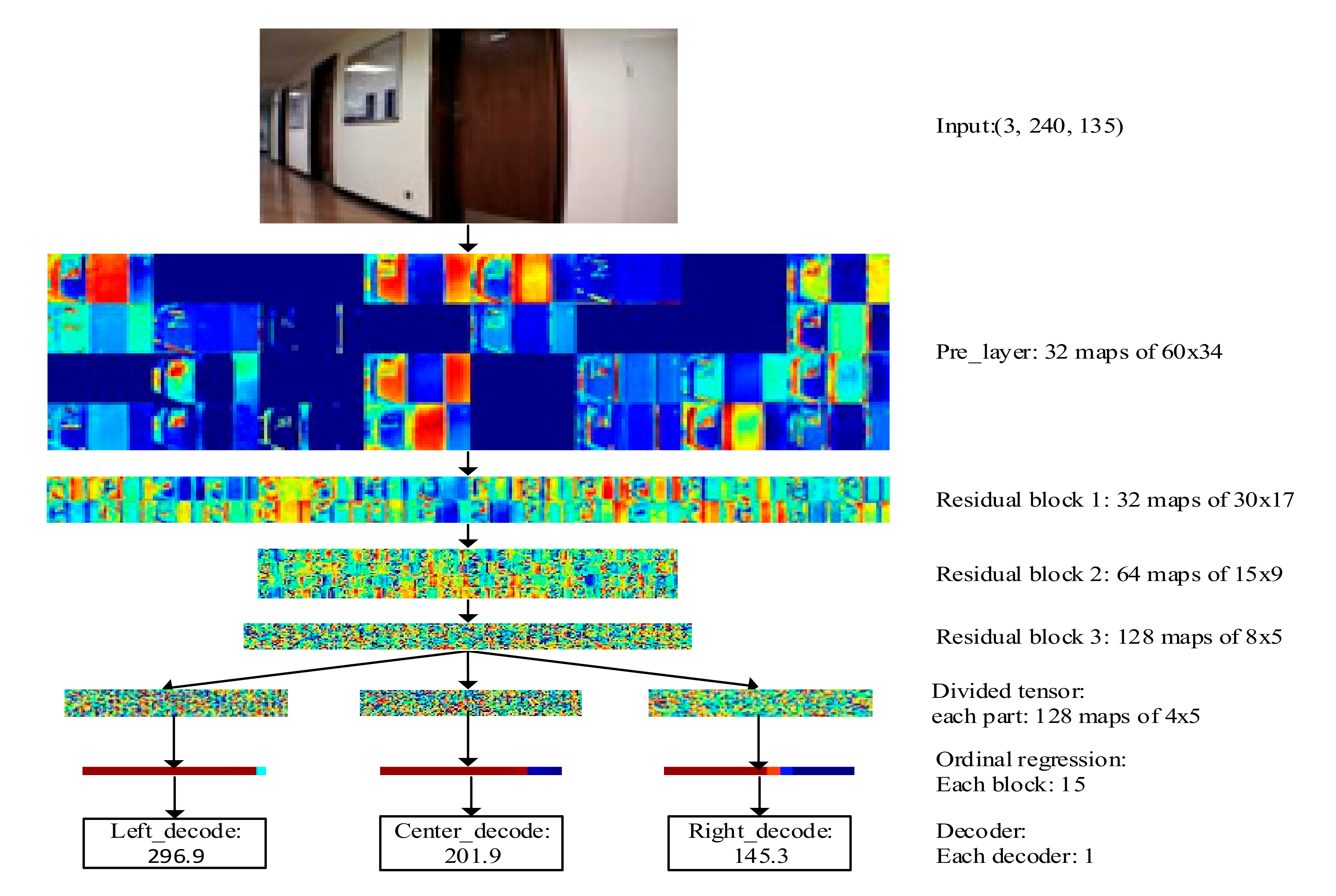
3.2. Network Structure

As it is distinct from methods which divide the original map before extracting feature maps [14,21], the NSIDOR network (NSIDOR-net), as shown in Figure 2, divides the final feature map a 3 extracted by the convolutional network based on ResNet-8 [33]. θ is the parameter of the feature extractor that needs to be trained. Then, each feature map is divided into three overlapping windows along the width direction. After that, ordinal regression block is used to process the divided feature maps to obtain K binary classification results. Based on the classification results, the distance decoder infers the corresponding distance. Each block is described in detail below.
The data set is D S = x , y j j = 0 2 , where x represents the input image and y j j = 0 2 represents the ground true (GT) distance labels, corresponding to the left, center, and right parts of the input image. The label y j is discretized as l j = l j 0 , l j 1 , , l j K 1 , where D k is the starting position of the k -th interval.
The convolutional network consists of a pre-layer and three residual blocks, as shown in Figure 3. The second column in Figure 3c sequentially represents the kernel size of the relevant operation, the number of output channels, and the step size. Equations (4)–(8) detail the feature extraction process.
The pre-layer block shown in Figure 3a can be expressed by Equation (4).
a 0 = P σ N W 0 x
where W 0 is the weight matrix of convolution (CONV), N · represents batch normalization (BN) function [34], Maximum pool function is represented by P · . σ · is ReLU function as Equation (5).
𝜎 i = i , i 0 0 , i < 0
As shown in the Figure 3b, the residual block consists of a residual part and a direct mapping part (CONV3). Since the number of feature diagrams of the l -th residual block input a l and output a l + 1 is different, 1 × 1 CONV is used here to carry out dimensional upgrading. Detailed equations are shown below:
a l + 1 = h l a l + F l a l
h l a l = W 3 a l
F l ( a 1 ) = N l 3 ( W 2 𝜎 l 2 ( N l 2 ( W 1 𝜎 l 1 ( N l 1 ( a l ) ) ) ) )
where, h l · and F l ·   respectively represent the direct mapping and the residual part of the l -th block, l 1 , 2 , 3 , N l i · , and σ l i · represent the i -th BN function of the l -th residual block.
Before entering the ordinal regression block, the feature map is divided first, as shown in Figure 4a. The size of the feature maps a 3 is 128 , 8 , 5 , which represents the total number of channels of the feature maps, the width and height of each feature map in turn. We divide each feature map into three overlapping windows along the width dimension, as shown in Figure 4a. After the division is completed, the feature maps M can be obtained, and M = M 0 , M 1 , M 2 . M 0 , M 1 , M 2 represent the feature maps on the left, center, and right part, respectively.
where m j is a reshape vector of M j , and m = m 0 , m 1 , m 2 is the input vector of ordinal regression block. Z = f m , ψ is the ordinal output, where the size is 3 × K . The weight is ψ = φ 0 , φ 1 , φ 2 containing weight vector φ j = ϕ j 0 , ϕ j 1 , , ϕ j K 1 ,   j = 0 , 1 , 2 . The size of ϕ j k is equal to 128 4 5 . Z = Z 0 , Z 1 , Z 2 respectively stands for the output of the left, middle, and right parts of the image, where Z j = z j 0 , z j 1 , , z j K 1 , z j k   is the k ordinal output z j k = ϕ j k T m j . Then, we use the sigmoid function to calculate the predicted probability, P ^ j k , of each binary classification:
P ^ j k y j D k   = 1 1 + e z j k
The predicted label l ^ j k = 1 P ^ j k > α   can be obtained according to the predicted probability, in which α is a hyperparameter.
In the inference stage, we need to parse the estimated classification of the decision area into continuous depth values. Due to the inconsistency problem of ordinal regression prediction, the prediction performance is usually improved by adding constraints during training [29], but this problem cannot be eliminated. In order to reduce the impact of the inconsistency of ordinal regression prediction, we propose a distance decoder with penalty coefficients:
d ^ j = i = 0 K d D i + 1 · l ^ j i · ω i
where d D i + 1 = D i + 1 D i is the difference between two adjacent discrete thresholds, the penalty coefficient is ω i = 1 , i = 0 δ ω i 1 · u l ^ j i , i 1 , and the two functions are δ x = 1 , x 1 x , 0 < x < 1 and u l ^ j i = 1 2 , l ^ j i = 0 2 , l ^ j i = 1 .
See the experimental Section 4.4 for the comparison between this distance resolver and the distance resolver in the literature [30].
In order to clearly show exemplary sizes at of vectors, matrices as data flow through the networks, we added an intermediate visualization, as shown in Figure 5. The left side of the figure is the last feature map of each block in the NSIDOR-Net, and the right side provides exemplary sizes of vectors. The data flow in the NSIDOR-Net is displayed clearly.
Compared with the algorithm presented in [14,21], the NSIDOR-net can not only share the weights of the convolution layers, which reduces the number of parameters, but can also classify different tasks into different regions, and thus the learning is more targeted. Compared with the algorithm presented in [35], an ordinal regression instead of binary classification is used to solve the monocular depth estimation for the indoor drone. The prediction distance is more refined [30]. To the best of our knowledge, this is the first work that uses ordinal regression to solve monocular depth estimation for an indoor drone.

3.3. Training

Due to the strong ordinal correlation of monocular depth information for indoor drones, the problem of estimating monocular depth for indoor drones is transformed into an ordinal regression problem, and ordinal loss is adopted to train the depth network parameters.
The loss function L θ , ψ of ordinal regression is the average value of the cross-entropy loss function L j θ , φ j for each part of each frame of the image:
L θ , ψ = 1 3 j = 0 2 L j θ , φ j
L j θ , φ j = k = 0 K 1 P j k log P ^ j k + 1 P j k log 1 P ^ j k
The derivation of the loss function L θ , ψ with respect to ϕ j k is as follows:
L θ , ψ ϕ j k = 1 3 j = 0 2 L j θ , φ j ϕ j k
L j θ , φ j ϕ j k = k = 0 K 1 P j k P ^ j k 1 P j k 1 P ^ j k P ^ j k 1 P ^ j k m j
The derivative formula of the loss function L θ , ψ with respect to the variable ϕ j k is derived from Equations (7) and (8) as follows:
L θ , ψ ϕ j k = 1 3 j = 0 2 k = 0 K 1 P j k P ^ j k m j
The desktop servers with Intel Xeon e5-2640 processors, 64 GB of memory and four RTX2080ti GPUs, and the Pytorch framework is used for the design and training of the NSIDOR-Net.

4. Analysis of Experiments

In this section, the public data set of a monocular indoor drone [36] is introduced. In order to illustrate the effectiveness of NSIDORA, the performance of the algorithm is not only compared with the performance of the state-of-the-art two-stream ordinal regression [14], but is also compared with the performance of another similar algorithm, ordinal regression based on NUD. The NUD-based ordinal regression is composed of an NUD strategy and the NSIDOR-net structure. It is different from NSIDORA only in terms of the discrete method relating to the decision area. The performance of the algorithms is compared in different aspects, including the overall performance (the root-mean-square error (RMSE) in the decision area, the classification performance in the non-decision area, and the inference frame per second (fps) of the algorithms), the selection of the number of discrete intervals, the performance comparison of the distance decoder, and the qualitative prediction result performance.

4.1. Data Set

We adopted the public data set presented in [36], which is a part of the data set from a prior study [14] that has been cleaned and verified to focus on indoor corridors. The data set contains 288 trajectories of nearly 54,600 frames, of which 52,989 images are labeled. We randomly selected 90% of the labeled images as the training set, 5% as the validation set during training, and the other 5% as the test set for the trained model. In order to ensure the comparability of algorithms, all algorithms adopted the same training set and test set. Figure 6 shows some of the training data. The numbers marked below the image represent the left, middle, and right overlapping areas of the closest distance between the UAV and the obstacle.

4.2. The Overall Performance Comparison

The comparison of the overall performance of the four algorithms is shown in Table 1. It can be seen from Table 1 that the classification performance of NSIDORA in the non-decision area is similar to the NUD-based algorithm. The RMSE (the lower the better) of NSIDORA in the decision area is 33.5% lower than that of the NUD-based ordinal regression, and is 6% higher than that of the state-of-the-art two-stream regression algorithm; however, it is better than that of two-stream regression in the first ten categories, shown in Figure 7 and Table 2. Furthermore, on a hardware device with an Intel Xeon E5-2640v4 32GB RAM, the inference fps of NSIDORA, another important indicator of drone indoor depth estimation [35], can reach 75, which is 3.4 times faster than that of the two-stream regression algorithm.
The RMSE comparison in each discrete segment of the distance prediction in the decision area of the four algorithms is shown in Figure 7. It can be seen in the Figure 7 that in the first 10 categories, the RMSE of NSIDORA was able to achieve better performance than that of the state-of-the-art two-stream regression model; although the RMSE of NSIDORA in the last three discrete segments increased, this result is within the acceptable range, because the errors of NSIDORA and the state-of-the-art two-stream regression algorithm are in the same order of magnitude. Furthermore, it is in line with our design that the larger the degree of discretization, the higher the RMSE value.
In order to better view the performance of the four algorithms in the top 10 categories of the decision area, we presented the results in Table 2. The RMSE of NSIDORA in the top 10 categories of the decision area is 21.8% lower than that of the two-stream regression algorithm.

4.3. Choice of the Number of Discrete Intervals in the Estimation Model

In order to select a better discrete interval number, the RMSE performance of NSIDORA in the decision area with five different discrete interval numbers is compared, as shown in Figure 8. It can be seen in the Figure that as the number of discrete intervals increases, the model’s accuracy does not change much after reaching a certain discrete number. To this end, we have chosen to classify thirteen decision areas. Therefore, the final total classification number is fifteen.

4.4. Performance Comparison of Decoders

Compared with the distance decoder presented in [30], the distance decoder in Equation (10) considers the inconsistency which is inevitable in ordinal regression. To illustrate this problem, these two decoders are used to decode the output of the NSIDOR-net. The RMSE values of the decoders in the decision area are shown in Table 3. It can be seen from the Table 3 that the RMSE of our distance decoder in the decision area was 20.7% lower than that of the distance decoder presented in [30].

4.5. Depth Predicetion

In order to better represent the performance of each algorithm in actual scenarios, the prediction results of each algorithm for multiple test data are shown in Figure 9. The ground truth label is represented by the abbreviation GT, and the gray shading represents the optimal prediction result corresponding to the scene. Dangerous areas are represented by “danger”, and safe areas are represented by “safe”. Comparing the prediction results of (a) and (b), it can be seen that when the distance is closer, the prediction effect of NSIDORA is better than that of two-stream ordinal regression. As the distance increases, the prediction result of the two-stream algorithm is better. This is consistent with the conclusion of Figure 7. Based on observations of prediction results (c) and (d) of each algorithm for the dangerous area and the safe area, it can be seen that there is little difference, which is consistent with Table 1.

5. Conclusions

As can be seen from the above description, the proposed system has fewer requirements for drone; it requires that the drone is equipped with a front camera, can transmit images to the desktop, and can receive control signals from the desktop. In response to the particularities of indoor environments, this paper proposes an ordinal regression algorithm based on NSID for monocular depth estimation for indoor drones. The experimental results show that the RMSE of NSIDORA in the decision area is 33.5% lower than that of the NUD-based ordinal regression method. Although the RMSE is higher than that of the state-of-the-art two-stream regression algorithm, the inference speed of NSIDORA is 3.4 times faster than that of two-stream ordinal regression method. Furthermore, the RMSE of our distance decoder in the decision area is 20.7% lower than that of the distance decoder presented in [30]. A common method is used in this article to show the performance of NSIDORA. However, the actual flight time and flight distance of the UAV are related not only to the prediction performance of the model, but also to the control algorithm. To this end, our next job is to design a deep learning controller to ensure that the drone can fly farther.

Author Contributions

Conceptualization, X.Z. and L.Z.; investigation, methodology, writing—original draft, X.Z.; review and editing, L.Z.; supervision, F.L.L.; funding acquisition, H.P. All authors have read and agreed to the published version of the manuscript.

Funding

This work was supported by the Scientific Instruments Development Program of NSFC (Grant/Award Number: 615278010); and by the Science and Technology Planning Project of Guangdong, China (Grant/Award Number: 2017B010116005).

Acknowledgments

The authors would like to thank MDPI (https://www.mdpi.com/authors/english) for English language editing. The authors would like to thank the Intelligent Digital Systems Laboratory (iDSL) at Imperial College London for providing the experimental data.

Conflicts of Interest

The authors declare no conflict of interest.

References

  1. Shakhatreh, H.; Sawalmeh, A.H.; Al-Fuqaha, A.; Dou, Z.; Almaita, E.; Khalil, I.; Othman, N.S.; Khreishah, A.; Guizani, M. Unmanned Aerial Vehicles (UAVs): A Survey on Civil Applications and Key Research Challenges. IEEE Access 2019, 7, 48572–48634. [Google Scholar] [CrossRef]
  2. Silvagni, M.; Tonoli, A.; Zenerino, E.; Chiaberge, M. Multipurpose UAV for search and rescue operations in mountain avalanche events. Geomat. Nat. Hazards Risk 2017, 8, 18–33. [Google Scholar] [CrossRef] [Green Version]
  3. Deng, C.; Wang, S.; Huang, Z.; Tan, Z.; Liu, J. Unmanned aerial vehicles for power line inspection: A cooperative way in platforms and communications. J. Commun. 2014, 9, 687–692. [Google Scholar] [CrossRef] [Green Version]
  4. Lee, K.H. Improvement in Target Range Estimation and the Range Resolution Using Drone. Electronics 2020, 9, 1136. [Google Scholar] [CrossRef]
  5. Choi, S.Y.; Cha, D. Unmanned aerial vehicles using machine learning for autonomous flight. Adv. Robot. 2019, 33, 265–277. [Google Scholar] [CrossRef]
  6. Carrio, A.; Sampedro, C.; Rodriguez-Ramos, A.; Campoy, P. A review of deep learning methods and applications for unmanned aerial vehicles. J. Sens. 2017, 2017, 3296874. [Google Scholar] [CrossRef]
  7. Scherer, S.A.; Zell, A. Efficient onbard RGBD-SLAM for autonomous MAVs. In Proceedings of the 2013 IEEE/RSJ International Conference on Intelligent Robots and Systems (IROS), Tokyo, Japan, 3–8 November 2013; pp. 1062–1068. [Google Scholar]
  8. Mei, C.; Sibley, G.; Cummins, M.; Newman, P.; Reid, I. RSLAM: A System for Large-Scale Mapping in Constant-Time using Stereo. Int. J. Comput. Vis. 2011, 94, 198–214. [Google Scholar] [CrossRef] [Green Version]
  9. Checchin, P.; Gerossier, F.; Blanc, C.; Chapuis, R.; Trassoudaine, L. Field and Service Robotics; Springer: Berlin/Heidelberg, Germany, 2009; pp. 151–161. [Google Scholar]
  10. Shen, S.; Mulgaonkar, Y.; Michael, N.; Kumar, V. Multi-sensor fusion for robust autonomous flight in indoor and outdoor environments with a rotorcraft mav. In Proceedings of the 2014 IEEE International Conference on Robotics and Automation (ICRA), Hong Kong, China, 31 May–7 June 2014; pp. 4974–4981. [Google Scholar]
  11. Alvarez, H.; Paz, L.; Sturm, J.; Cremers, D. Collision avoidance for quadrotors with a monocular camera. In Experimental Robotics; Springer: Berlin/Heidelberg, Germany, 2016; Volume 109, pp. 195–209. [Google Scholar]
  12. Daftry, S.; Zeng, S.; Khan, A.; Dey, D.; Melik-Barkhudarov, N.; Bagnell, J.A.; Hebert, M. Robust monocular flight in cluttered outdoor environments. arXiv 2016, arXiv:1604.04779. [Google Scholar]
  13. De Croon, G.; de Wagter, C. Challenges of Autonomous Flight in Indoor Environments. In Proceedings of the 2018 IEEE/RSJ International Conference on Intelligent Robots and Systems (IROS), Madrid, Spain, 1–5 October 2018; pp. 1003–1009. [Google Scholar]
  14. Kouris, A.; Bouganis, C.-S. Learning to Fly by MySelf: A Self-Supervised CNN-based Approach for Autonomous Navigation. In Proceedings of the 2018 IEEE/RSJ International Conference on Intelligent Robots and Systems (IROS), Madrid, Spain, 1–5 October 2018; pp. 1–9. [Google Scholar]
  15. Meng, K.; Li, D.; He, X.; Liu, M.; Song, W. Real-Time Compact Environment Representation for UAV Navigation. Sensors 2020, 20, 4976. [Google Scholar] [CrossRef] [PubMed]
  16. Ross, S.; Melik-Barkhudarov, N.; Shankar, K.S.; Wendel, A.; Dey, D.; Bagnell, J.A.; Hebert, M. Learning monocular reactive uav control in cluttered natural environments. In Proceedings of the 2013 IEEE International Conference on Robotics and Automation (ICRA), Karlsruhe, Germany, 6–10 May 2013; pp. 1765–1772. [Google Scholar]
  17. Kim, D.K.; Chen, T. Deep neural network for real-time autonomous indoor navigation. arXiv 2015, arXiv:1511.04668. [Google Scholar]
  18. Imanberdiyev, N.; Fu, C.; Kayacan, E.; Chen, I. Autonomous navigation of uav by using real-time model-based reinforcement learning. In Proceedings of the 2016 14th International Conference on Control, Automation, Robotics and Vision (ICARCV), Phuket, Thailand, 13–15 November 2016. [Google Scholar]
  19. Sadeghi, F.; Levine, S. Cad2rl: Real single-image flight without a single real image. arXiv 2016, arXiv:abs/1611.04201. [Google Scholar]
  20. Zhu, Y.; Mottaghi, R.; Kolve, E.; Lim, J.J.; Gupta, A.; Fei-Fei, L.; Farhadi, A. Target-driven visual navigation in indoor scenes using deep reinforcement learning. In Proceedings of the 2017 IEEE International Conference on Robotics and Automation (ICRA), Singapore, 29 May–3 June 2017; pp. 3357–3364. [Google Scholar]
  21. Gandhi, D.; Pinto, L.; Gupta, A. Learning to fly by crashing. In Proceedings of the 2017 IEEE/RSJ International Conference on Intelligent Robots and Systems (IROS), Vancouver, BC, Canada, 24–28 September 2017; pp. 3948–3955. [Google Scholar]
  22. Loquercio, A.; Maqueda, A.I.; del-Blanco, C.R.; Scaramuzza, D. DroNet: Learning to Fly by Driving. IEEE Robot. Autom. Lett. 2018, 3, 1088–1095. [Google Scholar] [CrossRef]
  23. Giusti, A.; Guzzi, J.; Ciresan, D.C.; He, F.-L.; Rodriguez, J.P.; Fontana, F.; Faessler, M.; Forster, C.; Schmidhuber, J.; di Caro, G.; et al. A machine learning approach to visual perception of forest trails for mobile robots. IEEE Robot. Autom. Lett. 2016, 1, 661–667. [Google Scholar] [CrossRef] [Green Version]
  24. Smolyanskiy, N.; Kamenev, A.; Smith, J.; Birchfield, S. Toward low-flying autonomous mav trail navigation using deep neural networks for environmental awareness. In Proceedings of the 2017 IEEE/RSJ International Conference on Intelligent Robots and Systems (IROS), Vancouver, BC, Canada, 24–28 September 2017. [Google Scholar]
  25. Yang, S.; Konam, S.; Ma, C.; Rosenthal, S.; Veloso, M.; Scherer, S. Obstacle avoidance through deep networks based intermediate perception. arXiv 2017, arXiv:1704.08759. [Google Scholar]
  26. Chakravarty, P.; Kelchtermans, K.; Roussel, T.; Wellens, S.; Tuytelaars, T.; van Eycken, L. CNN-based single image obstacle avoidance on a quadrotor. In Proceedings of the 2017 IEEE International Conference on Robotics and Automation (ICRA), Singapore, 29 May–3 June 2017; pp. 6369–6374. [Google Scholar]
  27. Niu, Z.; Zhou, M.; Wang, L.; Gao, X.; Hua, G. Ordinal regression with multiple output CNN for age estimation. In Proceedings of the IEEE Conference on Computer Vision and Pattern Recognition (CVPR), Las Vegas, NV, USA, 27–30 June 2016; pp. 4920–4928. [Google Scholar]
  28. Cao, W.; Mirjalili, V.A.; Raschka, S. Consistent rank logits for ordinal regression with convolutional neural networks. arXiv 2019, arXiv:abs/1901.07884. [Google Scholar]
  29. Liu, Y.; Kong, A.W.K.; Goh, C.K. A constrained deep neural network for ordinal regression. In Proceedings of the IEEE Conference on Computer Vision and Pattern Recognition (CVPR), Salt Lake City, UT, USA, 18–23 June 2018; pp. 831–839. [Google Scholar]
  30. Fu, H.; Gong, M.; Wang, C.; Batmanghelich, K.; Tao, D. Deep ordinal regression network for monocular depth estimation. In Proceedings of the IEEE Conference on Computer Vision and Pattern Recognition (CVPR), Salt Lake City, UT, USA, 18–23 June 2018; pp. 2002–2011. [Google Scholar]
  31. Gutiérrez, P.A.; Pérez-Ortiz, M.; Sánchez-Monedero, J.; Fernández-Navarro, F.; Hervás-Martínez, C. Ordinal regression methods: Survey and experimental study. IEEE Trans. Knowl. Data Eng. 2016, 28, 127–146. [Google Scholar]
  32. Li, X.; Wang, M.; Fang, Y. Height estimation from single aerial images using a deep ordinal regression network. IEEE Geosci. Remote Sens. Lett. 2020. [Google Scholar] [CrossRef]
  33. He, K.; Zhang, X.; Ren, S.; Sun, J. Identity Mappings in Deep Residual Networks. In Computer Vision—(ECCV) 2016—14th European Conference; Leibe, B., Matas, J., Sebe, N., Welling, M., Eds.; Springer: Amsterdam, The Netherlands, 2016; pp. 630–645. [Google Scholar]
  34. Ioffe, S.; Szegedy, C. Batch normalization: Accelerating deep network training by reducing internal covariate shift. In Proceedings of the 32nd International Conference on Machine Learning (ICML), Lille, France, 6–11 July 2015; pp. 448–456. [Google Scholar]
  35. Zhang, X.; Zhang, L.; Pei, H.; Lewis, F.L. Part-based multi-task deep network for autonomous indoor drone navigation. Trans. Inst. Meas. Control 2020. [Google Scholar] [CrossRef]
  36. Indoor Navigation UAV Dataset. Available online: https://www.imperial.ac.uk/intelligent-digital-systems/indoor-uav-data/ (accessed on 22 September 2020).
Figure 1. Discretization strategy diagram. (a) Uniform discretization (UD) [30]. (b) Non-uniform discretization (NUD). (c) Non-uniform spacing-increasing discretization (NSID) discretizing the depth interval D 0 , D 7 into seven intervals.
Electronics 09 01767 g001
Figure 2. The non-uniform spacing-increasing discretization-based ordinal regression (NSIDOR)-net framework.
Electronics 09 01767 g002
Figure 3. The convolutional network. (a) Pre-layer. (b) Residual block. (c) Sub-nets table.
Electronics 09 01767 g003
Figure 4. Detail blocks. (a) Division. (b) Ordinal regression block.
Electronics 09 01767 g004
Figure 5. Intermediate visualization of NSIDOR-net.
Electronics 09 01767 g005
Figure 6. Training data set.
Electronics 09 01767 g006
Figure 7. Root-mean-square error (RMSE) comparison of the algorithms in the decision region.
Electronics 09 01767 g007
Figure 8. RMSE in the decision area corresponding to different discrete intervals.
Electronics 09 01767 g008
Figure 9. The prediction results of each algorithm on the actual scene.
Electronics 09 01767 g009
Table 1. Performance comparison of algorithms.
AreaPerformanceAlgorithms
NUD-Based Ordinal RegressionNSIDORA (ours)Two-Stream [14]
Dangerousaccuracy0.9774757770.977979112-
Precision0.9616144570.9470329-
Recall0.9453031850.94556296-
F1-Score0.9533671470.946273898-
DecisionRMSE0.03220.02140.0201
Safeaccuracy0.9950924880.990184976-
Precision0.9370248960.94399412-
Recall0.955133240.93809859-
F1-Score0.9454893770.940682157-
-fps757522
Table 2. The RMSE of the four algorithms in the top 10 categories of the decision area.
AreaPerformanceAlgorithms
NUD-Based Ordinal RegressionNSIDORA (ours)Two-Stream [14]
DecisionRMSE0.03400.01540.0197
Table 3. The RMSE of the two decoders in the decision area.
AreaPerformanceDecoders
Decoder [30]Ours
DecisionRMSE0.02700.0214
Publisher’s Note: MDPI stays neutral with regard to jurisdictional claims in published maps and institutional affiliations.

