Abstract
The Band Collocation Problem appears in the context of problems for optimizing telecommunication networks with the aim of solving some concerns related to the original Bandpass Problem and to present a more realistic approximation to be solved. This problem is interesting to optimize the cost of networks with several devices connected, such as networks with several embedded systems transmitting information among them. Despite the real-world applications of this problem, it has been mostly ignored from a heuristic point of view, with the Simulated Annealing algorithm being the best method found in the literature. In this work, three Variable Neighborhood Search (VNS) variants are presented, as well as three neighborhood structures and a novel optimization based on Least Recently Used cache, which allows the algorithm to perform an efficient evaluation of the objective function. The extensive experimental results section shows the superiority of the proposal with respect to the best previous method found in the state-of-the-art, emerging VNS as the most competitive method to deal with the Band Collocation Problem.
1. Introduction
The evolution of optical communications in the last years has attracted the attention of the scientific community. Additionally, the quick expansion of the Internet of Things where the embedded systems in every kind of device must be connected has made traditional algorithms for solving problems derived from the transportation of digital data obsolete. These problems are now a real challenge for the most modern algorithms mainly due to the vast increase of network sizes. Most of these problems can be classified into two different types: finding the optimal route for the signal and reducing the costs of the equipment required to deploy and maintain the network [1]. This paper is focused on solving one of the most extended problems of the second type, the Band Collocation Problem [2].
The Band Collocation Problem cannot be defined without introducing the Bandpass Problem (BP). The BP was originally presented in Bell and Babayev [3]. One of the main objectives to take into account in the design of efficient networks is to minimize the cost of the equipment required to maintain it without deteriorating its quality. In order to do so, it is necessary to optimize the traffic flow to reduce the hardware involved in the process.
A network is conformed by a set of T target stations, with , that are connected with fiber-optic cables. Then, a source station transmits data to these target stations, which can be transported by different wavelengths , using a technology named dense wavelength division multiplexing (DWDM) in a single fiber optic cable [4]. It is worth mentioning that not all the target stations need to receive the data from all the wavelengths. A device named Add/Drop Multiplexer (ADM) is responsible for requesting the appropriate data from the fiber-optic cables at each station. The ADM uses a special card that controls the wavelengths required in each station. Some cards are able to receive all the data in consecutive wavelengths, so it is interesting to join in adjacent wavelengths all the data required by a single station. This structure conformed with consecutive wavelengths is named a Bandpass, and the number of consecutive wavelengths in a Bandpass is named as Bandpass number. Then, the objective of the BP is to select the optimal wavelength permutation that requires the minimum number of cards to be used in ADM for a given Bandpass number.
The BP was deeply analyzed in [5], while the dataset of instances for this problem was originally presented in [6]. The problem was proven to be -hard in [7] using a reduction for the Hamilton Problem for any Bandpass number. A game for understanding the permutations performed in the BP was also presented [8], which implements a mathematical model for solving it. Some specific configuration for networks can be solvable in linear time, such as those with just three columns [9]. Although the BP has attracted the focus of several works, see [10,11,12], the best results in the literature are obtained by [13,14].
The original BP formulation has become obsolete due to the continuous evolution of communication networks. Therefore, it is necessary to revise the original model to adapt it to the new advances. Notice that it is not a correction but an adaptation of the new technologies. In particular, the cards in the ADM can now filter all data, not only the one requested for the station, from consecutive wavelengths [15]. However, in the original problem, only the data requested for the station can be filtered. In new ADMs, more than one card can be used now, and the Bandpass number may be a power of two. Furthermore, the original BP does not evaluate the cost of the cards since it considers just a single type of card, while in the real application several different cards can be used. Thus, the cost must be taken into account for evaluating the quality of a solution.
The inclusion of all these new features result in a new problem called the Band Collocation Problem (BCP). In this problem, an ADM located at a target station can filter data even if it is transmitted to a different target station. The Bandpass number can vary in the same model, always being a power of two. Finally, the cost of each Bandpass number is different.
The network is represented with a binary matrix , with and , where n and m are the number of target stations (columns) and the number of wavelengths (rows), respectively. If data fragment i must be transmitted to target station j, the element is set to 1; otherwise, . Each band card is usually denoted with , with length and cost , where .
A solution of the BCP is usually represented as a permutation of the rows, , where each indicates which wavelength is located at row i. Then, the aim of this optimization problem is to find the permutation of rows that minimizes the sum of costs of all -Band cards used in the complete network. In mathematical terms:
where , , and is a binary variable that is set to 1 if row i is the first row of a -Band in column j; otherwise, . Notice that each data fragment in every target station must be covered by exactly one band. We refer the reader to [2] for a formal definition of the problem and a mathematical formulation.
Figure 1 shows the representation of two different solutions for the BCP for a network with a single source station , three target stations(named , and ), and five wavelengths (named , , , , and ). In each target station, the data fragment that is requested is colored in black. In particular, requires data from wavelengths and ; requires data from and ; and from and . The costs for the cards are for , for , and for .
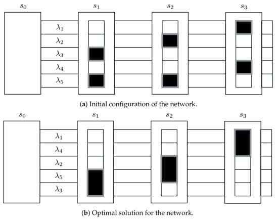
Figure 1.
Initial and optimal configuration for a given set of 5 wavelengths and 3 target stations.
Figure 1a depicts the initial configuration of the network, where the wavelengths have been included in lexicographical order (i.e., from to ). The wavelengths that have been grouped in the same card are highlighted with a thick grey border (with length ). Then, the initial cost of the network is evaluated as .
If we now analyze Figure 1b, the wavelengths have been set in a different ordering . Due to this permutation, it is now possible to group more than one wavelength in the same card, resulting in a total cost of (i.e., with three band cards of size ). Therefore, the ordering results in a better solution than the initial configuration .
Since the BCP has been recently proposed, it has not been widely studied yet. The first approach for solving the BCP is a fast heuristic algorithm [16], while the first exact algorithm is a binary integer programming model, which is solved with GAMS and CPLEX [17]. On the contrary, the first heuristic approach for the BCP is a classical Genetic Algorithm [18]. Then, the same authors developed several bioinspired algorithms for further improving the results obtained [2], but the results obtained were not satisfactory. In particular, a new Genetic Algorithm (GA), a Simulated Annealing (SA), an Artificial Bee Colony (ABC) algorithm are proposed. Additionally, a 0–1 integer model for the BCP is presented for solving small instances to verify the quality of the heuristic proposal. The detailed comparison provided by the author shows that the best method in the literature for the BCP is Simulated Annealing.
In this paper, we propose a novel approach based on the Variable Neighborhood Search (VNS) methodology [19,20] to deal with BCP. First of all, we introduce an extremely efficient strategy (in both, computing time and memory requirements) to evaluate the objective function. Then, we propose three different greedy constructive procedures to start the search from promising regions in the search space. Additionally, we define three different neighborhood structures and three local search methods (each one based on a different neighborhood). Finally, all these strategies are embedded within three VNS variants (e.g., Basic VNS, Variable Neighborhood Descent, and General VNS).
The main contributions of this work are:
- A new dynamic programming algorithm for evaluating the objective function value is proposed. This new method leverages the Least Recently Used cache structure to drastically reduce the complexity of the objective function evaluation, thus reducing the computational effort.
- Three Variable Neighborhood Search variants are proposed for analyzing the impact of intensification and diversification in the context of the Band Collocation Problem.
- Three constructive procedures are presented, each one of them using different properties of the solution structure to generate initial solutions.
- Three neighborhoods are defined, which allow us to explore the solution space through different approaches.
The remaining of the paper is structured as follows: Section 2 describes the optimization proposed to increase the performance in the evaluation of the objective function. Section 3 presents the algorithmic proposal of this work. Section 4 is devoted to select the best configuration for the proposed algorithm and analyzes the results obtained when comparing it with the best previous method found in the state-of-the-art. Finally, Section 5 draws some conclusions derived from the research.
2. Evaluation of the Objective Function
Given a solution of the BCP, representing a permutation of wavelengths, the selection of the optimal combination of cards to minimize the cost associated to that permutation is a highly computationally demanding task. Specifically, it is necessary to test every possible combination of cards and select the one with the minimum cost. Indeed, it is mandatory to evaluate all card combinations since, otherwise, we can miss high quality solutions or even the optimum.
In order to reduce the computational effort, the author of [21] proposes a Dynamic Programming (DP) algorithm that memorizes the already explored solutions to reduce the computing time for finding the minimum cost. In particular, they consider each column as a subproblem, solving it with the DP method, memorizing during the search the solutions found. The complexity of the method is .
In this work, we propose an improvement to this evaluation by increasing the number of elements memorized during the DP for reducing the total computing time. This behavior leads the procedure to require a large amount of memory (more than 32 GB RAM). In general, these hardware requirements are not available. Therefore, we propose a new memory structure, by using the Least Recently Used (LRU) algorithm, which allow overhead high performance buffer management replacement [22]. This optimization strategy is able to keep in memory just the strictly necessary data, drastically reducing the required memory. It is totally scalable, adapting the memory requirements to the available memory in the computer.
The algorithm stores the memorized information (in the Dynamic Programming procedure) in a table (implemented with a hash map). Each table entry additionally stores information about the immediately less and more used element in the table with respect to itself. Therefore, when the table is complete and a new element must be stored, the algorithm replaces the least used element, updating it. If the table is rather small, the cache will be frequently updated, affecting the performance of the evaluation of the objective function (i.e., the larger the table, the faster the algorithm). Figure 2 shows a graphical example of the LRU cache structure.
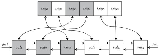
Figure 2.
Graphical illustration of the Least Recently Used (LRU) cache optimization structure.
The structure depicted in the upper side of the figure represents the table where keys are stored. Similarly, in the lower side a double linked list is depicted, which stores the values in ascending order with respect to the last time it was accessed. In particular, in this example the keys , and are linked with the corresponding entries, i.e., , , and . For the sake of clarity, we have highlighted in grey these pairs of keys and values. Notice that, using the appropriate data structures, the complexity of inserting and deleting a new element in the table is .
3. Variable Neighborhood Search
Variable Neighborhood Search (VNS) is a metaheuristic [23], which was originally proposed as a general framework for solving hard optimization problems. The main contribution of this methodology is to consider several neighborhoods during the search and to perform systematic changes in the neighborhood structures. Although it was originally presented as a simple metaheuristic, VNS has drastically evolved, resulting in several extensions and variants: Basic VNS, Reduced VNS, Variable Neighborhood Descent, General VNS, Skewed VNS, Variable Neighborhood Decomposition Search, or Variable Formulation Search, among others. See [19,20,24] for a deep analysis of each variant. In this work, we propose a comparison among the most extended variants of VNS: Basic Variable Neighborhood Search (BVNS), Variable Neighborhood Descent (VND), and General Variable Neighborhood Search (GVNS).
3.1. Basic VNS
This variant combines deterministic and random changes of neighborhood structures in order to find a balance between diversification and intensification as presented in Algorithm 1.
| Algorithm 1 |
|
The algorithm receives as input parameters the matrix A and the largest neighborhood to be explored, . In step 1, an initial solution is generated by considering one of the constructive procedures presented in Section 3.4. Then, the solution is locally improved with one of the local search methods described in Section 3.5 (step 2). Starting from the first predefined neighborhood (step 3), BVNS iterates until reaching the maximum considered neighborhood (steps 4–8). For each iteration, the incumbent solution is perturbed with the shake method (step 5). This method is designed to escape from local optima by randomly exchanging the position of k wavelengths, generating a solution in the neighborhood under exploration. The local search method is then responsible for finding a local optimum in the current neighborhood with respect to the perturbed solution . Finally, the neighborhood change method selects the next neighborhood to be explored (step 7). In particular, if outperforms in terms of the objective function value, then it is updated (i.e., ), and the search starts again from the first neighborhood (i.e., ). Otherwise, the search continues in the next neighborhood (i.e., ). The algorithm stops when reaching the largest considered neighborhood , returning the best solution found during the search (step 9).
3.2. Variable Neighborhood Descent
This variant performs the changes in the neighborhood structure in a totally deterministic manner. Specifically, the diversification part of VNS is completely removed, focusing in the intensification phase. Algorithm 2 shows the pseudocode of the VND algorithm.
| Algorithm 2 |
|
The algorithm receives an input solution and a set of neighborhoods to be explored. The proposed VND follows the sequential Basic VND scheme described in [25]. Starting from the first neighborhood (step 1), the algorithm explores following a sequential ordering. In particular, for each neighborhood , VND finds a local optimum with respect to the neighborhood under exploration (step 3). Then, the neighborhood change method (step 4) resorts to the first predefined neighborhood if and improvement is found (), otherwise continuing with the next neighborhood (). The method ends when no improvement is found in any of the considered neighborhoods, returning the best solution found.
Notice that the final solution is a local minimum with respect to all the considered neighborhoods . Then, reaching a global optimum is more probable than when considering a single neighborhood structure.
3.3. General VNS
This variant combines BVNS and VND with the aim of balancing intensification and diversification for providing even better solutions. Specifically, the General VNS replaces the local search phase of BVNS with a complete VND algorithm. This modification allows GVNS to find better solutions in the improvement phase, thus increasing the probability of reaching a global optimum.
The main drawback of GVNS lies in the computing time required by the VND phase, which can eventually lead to a very computationally demanding algorithm. However, the efficient implementation of the objective function evaluation described in Section 2 counteracts that disadvantage of GVNS (see Section 4 for a thorough analysis of the performance).
For the sake of brevity, we do not provide the pseudocode for this variant since it consists of replacing step 6 from Algorithm 1 with the following sentence:
with VND the variant described in Algorithm 2. Furthermore, the input parameter of GVNS is the set of neighborhoods instead of the maximum neighborhood to be explored .
3.4. Constructive Procedure
In the context of VNS, the initial solution can be generated at random, but several recent works have concluded that using an initial high quality solution leads the algorithm to converge faster than when starting from a random initial solution (see [26,27,28,29,30,31], for some successful results).
This work presents three different greedy constructive procedures that are able to find a high quality solution in negligible computing times. Section 4 will discuss the results obtained with each constructive procedure to select the most adequate one for the complete VNS framework. The three constructive procedures follows the same greedy scheme but varying the greedy function used to select the next wavelength to be included in the solution.
The first constructive procedure, named , is based on the idea that wavelengths that are required in similar target stations should be located consecutively. In particular, the method starts from an empty solution and generates a solution starting from a given wavelength. Once the first wavelength has been selected, the next wavelength to be considered would be the one with the maximum number of target stations in common with the previous one. Let be a partial solution of the BCP, be the wavelength located in row i, and j be the target station. We then define the score as:
More formally, the greedy function value for a given wavelength is calculated as:
where if and only if the wavelength i must be transmitted to target station j. Then, the next wavelength to be included in the solution under construction is evaluated as:
The method iterates until all the wavelengths have been included in the solution. Since the first wavelength selected is a key part in the constructive procedure, it generates a solution starting in each available (i.e., m solutions are constructed), returning the best solution in terms of objective function value.
The second constructive method, , modifies the definition of the score. In this case, the score evaluates the number of target stations for which the wavelength under consideration is not necessary. More formally:
Analogously, the definition of and are computed in a similar way than and but replacing with .
Finally, the last constructive method, considers both, the number of target stations that two wavelengths have in common and those for which the wavelength is not required, resulting in the score . In mathematical terms:
Similarly, and are computed. Notice that the proposed constructive procedures are extremely fast since they do not need to evaluate the objective function during the construction, but a single evaluation after constructing the solution.
3.5. Neighborhood Structures
A neighborhood N for a given solution is defined as the set of solutions that can be reached from by performing a single movement. Therefore, before defining a neighborhood structure it is necessary to introduce the movements that are considered in this work.
The first movement consists in exchanging the position of two given wavelengths i and , with . Given a solution , the move results in a new solution where the wavelengths i and have exchanged original positions.
The second movement is based on insertions. In this case, inserting a wavelength i in a position , with extracts i from its original position in solution , and inserts it in the position of wavelength , displacing the wavelengths located in the range given by the position of wavelength i and position of wavelength . More formally, given a solution , the move results in solution .
The third and last movement is based on the move, which is a widely used operator in vehicle routing problems [32]. In that context, given a route, the move reverses a certain part of the route. The adaptation to the BCP is performed as follows. Given a solution , the movement reverses all the wavelengths located in positions between and , resulting in solution .
Once the movements have been defined, we can now define the neighborhoods considered in this work. Specifically, we define , , and for neighborhoods based on swaps, insertions, and , respectively, as:
For each neighborhood structure, we propose a local search method, which locally improves the input solution. A local search is conformed with the neighborhood to be explored and the order in which those neighbor solutions are traversed. In particular, we propose three local search methods, namely , , and . All of them follows the same ordering when exploring the associated neighborhood. The search starts performing the movement over the wavelengths located at the first and second positions of the solution, continuing in ascending order until the complete neighborhood is explored. It is worth mentioning that the three proposed local search methods follow a first improvement approach, which usually leads to better results [33]. In this scheme, the first movement that leads to a better solution is performed, restarting the search. The search stops when no improvement is found after exploring the complete neighborhood.
4. Computational Results
This section has two main objectives: to select the best combination of parameter values for the proposed algorithms, and to perform an in-depth comparison of the proposed algorithm and the best method found in the state-of-the-art. All the algorithms have been implemented in Java 11 and the experiments have been performed in an AMD Ryzen 53,600 (2.2 GHz) with 16 GB RAM.
Since the BCP have been recently proposed, there are not many research works on this problem. In particular, the best method found in the literature is the Simulated Annealing (SA) algorithm proposed in [2], which is able to outperform the results obtained with the Genetic Algorithm, and the Artificial Bee Colony algorithm also presented in that work. Therefore, we will compare our best proposal with the SA procedure.
In order to have a fair comparison, we have considered the same set of instances than the ones used in the previous work. It is called the BPLIB and it is publicly available at http://grafo.etsii.urjc.es/bcp. We select the same set of instances used in [2], which consists in 72 matrices with m ranging from 12 to 96 and n ranging from 6 to 28. In these instances the optimal value is not known and the best known value is the one obtained in [2].
This section is divided into two types of experiments. On the one hand, the preliminary experimentation is designed to find the best values for the input parameters of the proposed algorithms. In particular, it is required to perform the following analysis:
- Selection of the best constructive procedure among , , and .
- Selection of the best local search method among , , and .
- Selection of the neighborhood exploration order within VND, testing all possibilities.
- Selection of the best value for the Basic VNS algorithm among .
- Selection of the best value for the General VNS algorithm among .
- Selection of the best VNS algorithm for the BCP among Basic VNS, VND, and General VNS.
On the other hand, the competitive testing has the aim of analyzing the performance of the final version of the algorithm when comparing the results with the ones presented in the best method found in the literature. A subset of 15 out 72 representative instances (20%) are used in the preliminary experimentation to avoid overfitting. Then, in the competitive testing, the complete set of 72 instances is considered.
The metrics reported in all the experiments are: Avg., the average objective function value; Time(s), the computing time required by the algorithm to finish in seconds; Dev(%), the average deviation with respect to the best solution found in the experiment; and #Best, the number of times that the algorithm reaches the best solution of the experiment. For the sake of clarity, the best value of each metric is highlighted with bold font.
4.1. Preliminary Experimentation
The first preliminary experiment is intended to select the best constructive procedure among the ones presented in Section 3.4: , , . Table 1 shows the results obtained when executing each constructive procedure over the preliminary set of instances.

Table 1.
Comparison among the three constructive procedures , , .
As it can be seen, the computing time is negligible in all cases, being considerably smaller than 1 s. Hence, in terms of quality, emerges as the best constructive method with the largest number of best solutions found, missing the best solution in only 5 out of 15 instances. Notice that, in those cases in which the best solution is not found, remains close to it, as it can be seen in the obtained average deviation of 0.12%. From this experiment we can derive that it is interesting to locate the wavelengths that must be delivered to the same target stations in close rows. Therefore, we select as the best constructive method and it will be used in the final competitive testing.
The next experiment is designed to evaluate the influence of each local search method (, , and ) when coupling it with the best constructive procedure . Table 2 shows the results obtained in this experiment.
Table 2.
Comparison among the three local search methods , , when improving the solutions generated by the best constructive procedure, .
It is worth mentioning that the efficient evaluation of the objective function allows the local search to be executed also in small computing times. In this case, the superiority of is clear, reaching the best solution in every instance, with a deviation of 0.00%. Then, is the local search selected for BVNS.
The aim of the third experiment is to find the optimal ordering of the neighborhood structures in the context of VND. Although it is usually recommended to firstly explore the neighborhoods from the smallest to the largest [34], we perform an empirical evaluation of all possibilities in order to select the best one. In this experiment, each variant of VND has been applied to the solution derived from . Figure 3 shows a graph comparing computing time (X-axis) with average deviation (Y-axis) of the six possibilities for the local search order within VND.
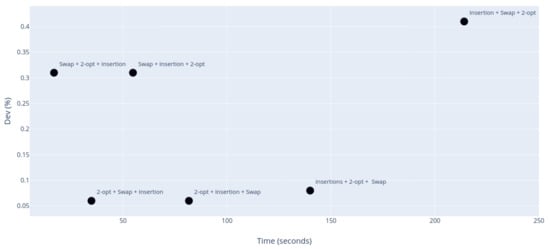
Figure 3.
Time versus deviation graph for the different orderings of the local search inside the Variable Neighborhood Descent (VND) framework.
As it can be derived from the graph, the two best options are and , with the same average deviation of 0.06%. Since the computing time of is twice the time of , we select the last one for the VND and GVNS algorithm.
The next experiment analyzes the influence of the parameter in the context of BVNS. The VNS literature [19] recommends using small values for this parameter. This is mainly because large values of will explore solutions that are very different to the incumbent one, being similar to constructing an entire new solution. Therefore, the values considered for this experiment are . Notice that, to favor scalability, the value of the parameter is dependent on the number of wavelengths m of the input instance. Table 3 shows the results obtained in this experiment.
Table 3.
Comparison of the different values considered in the Basic Variable Neighborhood Search (BVNS) algorithm.
As it can be observed in this experiment, the quality of the solutions increase with the value of . However, when reaching , the search seems to be stagnated, but increasing the computing time required. Therefore, we select for the final BVNS algorithm.
The next experiment is designed to identify the best value for the GVNS algorithm. Following the same reasoning as in the previous experiment, we have tested the same values, . Table 4 shows the results of this experiment.
Table 4.
Comparison of the different values considered in the General Variable Neighborhood Search (GVNS) algorithm.
Again, the larger the value of , the better the quality. However, the differences in quality (deviation and number of best solutions) between and are negligible, while the latter requires a larger computing time. Therefore, we select as the best value for GVNS.
The last preliminary experiment is intended to analyze which VNS variant is the most promising one. Table 5 shows the results obtained by the best configuration of each VNS variant: BVNS, VND, and GVNS.
Table 5.
Comparison among the different VNS variants for the preliminary set of instances.
As it can be derived from the data, the worst variant is BVNS, with a deviation of 2.04%. However, it is the fastest algorithm, so it would be an interesting selection when requiring small computing times. Analyzing the results of VND and GVNS, the former is considerably faster, as expected, since GVNS executes a complete VND in each iteration. However, it is worth mentioning that VND is able to reach a small deviation of 0.50%, which makes it a relevant candidate if the computing time is one of the main requisites, although it only reaches 2 out of 15 best solutions. Finally, GVNS emerges as the best variant reaching all the best solutions found, requiring a larger, but reasonable, computing time.
4.2. Competitive Testing
Once the parameters of the proposed algorithm have been tested, this competitive testing is devoted to analyzing the efficiency of the best variant, which is GVNS, with the best previous method found in the state-of-the-art, which is based on a Simulated Annealing (SA) framework. In this case, the experiment is performed over the complete set of 72 instances. The results of the previous method are directly imported from the original work [2]. Table 6 shows the summary table with the results obtained by both algorithms. To facilitate future comparisons, we report in Appendix A (see Table A1) individual results per instance.
Table 6.
Comparison with the state-of-the-art.
In order to have a fair comparison, we have considered the same experimental methodology than the one used in the previous paper. In particular, the algorithm has executed 50 independent iterations, reporting the average objective function value and time in the first main row, and the best values in the second main row.
If we firstly analyze the average results, we can clearly see that GVNS is able to obtain the largest number of best solutions (65 vs. 7) and a smaller deviation (0.04% vs. 1.10%). This small deviation indicates that, in the seven instances in which GVNS does not reach the best solution, it remains very close to it. Regarding the best results obtained with both algorithms, GVNS is still the best option, with the smallest deviation (0.19% vs. 0.57%) and the largest number of best solutions found (44 vs. 38). Notice that the computing times are equivalent in both cases. It is worth mentioning that it is always a difficult task to compare execution times of different algorithms implemented in different programming languages but, in this case, the execution environment could be considered equivalent.
In order to confirm that there are statistically significant differences between both algorithms, we have conducted a non-parametric pairwise Wilcoxon test. The resulting p-value smaller than 0.05 confirms the superiority of our proposal.
5. Conclusions
This paper presents three Variable Neighborhood Search variants for dealing with the Band Collocation Problem. This problem arose in the context of telecommunication networks to solve some concerns with the original Bandpass Problem with respect to its practical application.
The evaluation of the objective function is very computationally demanding, so the proposed LRU cache optimization method is able to efficiently evaluate solutions without requiring large computational times. This optimization allows the VNS to perform a deeper analysis of the search space.
Three neighborhood structures are explored, as well as their combination in a Variable Neighborhood Descent scheme. Additionally, a Basic VNS, which considers the best neighborhood structure in its local search phase is presented, as well as a General VNS algorithm, which increases the diversification of VND. The experimental results show how the combination of several neighborhood structures in the GVNS scheme allows the algorithm to explore a wider portion of the search space, resulting in better results.
Finally, the General VNS algorithm is able to outperform the state-of-the-art method, based on Simulated Annealing in similar computing times, emerging GVNS as a competitive method for the Band Collocation Problem.
Author Contributions
I.L.-O. implemented the proposed algorithm, and performed the experiments; A.D. and J.S.-O. designed the algorithm and the experiments; A.D. and M.Á.R.-G. analyzed the data and contributed reagents/materials/analysis tools; A.D., I.L.-O. and J.S.-O. wrote the paper. All authors have read and agreed to the published version of the manuscript.
Funding
This research was funded by “Ministerio de Ciencia, Innovación y Universidades” under grant ref. PGC2018-095322-B-C22, “Comunidad de Madrid” and “Fondos Estructurales” of the European Union with grant references S2018/TCS-4566, Y2018/EMT-5062, and PEJD-2019-PRE/TIC-16151, and by Research Talent Attraction Program by the Comunidad de Madrid with grant reference 2017-T2/TIC-5664.
Acknowledgments
Authors would like to thank researcher R. Martin-Santamaria for his promising ideas about the optimization of the objective function evaluation.
Conflicts of Interest
The authors declare no conflict of interest.
Appendix A
Table A1 shows the results of our competitive testing, where we report for each instance the objective function value (O.F.), the average deviation with respect to the best known value (Dev (%)), an indicator that determines whether the methods match the best known solution or not (#Best), and the computing time in seconds (Time (s)). These results are obtained as the average execution of 50 independent iterations (Average (grey)) or best one among those 50 iterations (Best).
Table A1.
Individual result for each instance.
Table A1.
Individual result for each instance.
| SA | GVNS | |||||||||||||||
|---|---|---|---|---|---|---|---|---|---|---|---|---|---|---|---|---|
| Average | Best | Average | Best | |||||||||||||
| Name | O.F. | Dev (%) | #Best | Time (s) | O.F. | Dev (%) | #Best | Time (s) | O.F. | Dev (%) | #Best | Time (s) | O.F. | Dev (%) | #Best | Time (s) |
| T1-M1-R10 | 23,144 | 0.02 | 0 | 0.85 | 23,140 | 0.00 | 1 | 42.50 | 23,140 | 0.00 | 1 | 0.04 | 23,140 | 0.00 | 1 | 0.37 |
| T1-M1-R30 | 19,670 | 0.05 | 0 | 0.85 | 19,660 | 0.00 | 1 | 42.50 | 19,660 | 0.00 | 1 | 0.02 | 19,660 | 0.00 | 1 | 0.23 |
| T3-M1-R10 | 47,936 | 0.41 | 0 | 0.86 | 47,680 | 0.00 | 1 | 43.00 | 47,738 | 0.00 | 1 | 0.04 | 47,680 | 0.00 | 1 | 0.41 |
| T3-M1-R30 | 37,136 | 0.94 | 0 | 0.85 | 36,640 | 0.00 | 1 | 42.50 | 36,791 | 0.00 | 1 | 0.04 | 36,640 | 0.00 | 1 | 0.39 |
| T4-M1-R10 | 42,041 | 0.36 | 0 | 1.68 | 41,860 | 0.00 | 1 | 84.00 | 41,890 | 0.00 | 1 | 0.23 | 41,860 | 0.00 | 1 | 2.27 |
| T4-M1-R30 | 36,109 | 1.93 | 0 | 1.69 | 35,570 | 0.85 | 0 | 84.50 | 35,425 | 0.00 | 1 | 0.16 | 35,270 | 0.00 | 1 | 1.57 |
| T6-M1-R10 | 84,939 | 0.46 | 0 | 1.72 | 84,530 | 0.00 | 1 | 86.00 | 84,549 | 0.00 | 1 | 0.12 | 84,530 | 0.00 | 1 | 1.19 |
| T6-M1-R30 | 63,827 | 0.24 | 0 | 1.69 | 63,270 | 0.00 | 1 | 84.50 | 63,672 | 0.00 | 1 | 0.10 | 63,270 | 0.00 | 1 | 0.91 |
| T7-M1-R10 | 76,710 | 0.51 | 0 | 3.83 | 76,070 | 0.00 | 1 | 191.50 | 76,323 | 0.00 | 1 | 1.44 | 76,240 | 0.22 | 0 | 14.35 |
| T7-M1-R30 | 63,983 | 1.49 | 0 | 3.84 | 62,790 | 0.45 | 0 | 192.00 | 63,045 | 0.00 | 1 | 2.06 | 62,510 | 0.00 | 1 | 20.58 |
| T9-M1-R10 | 155,409 | 0.37 | 0 | 3.97 | 154,410 | 0.00 | 1 | 198.50 | 154,837 | 0.00 | 1 | 1.61 | 154,410 | 0.00 | 1 | 16.10 |
| T9-M1-R30 | 112,506 | 1.00 | 0 | 3.93 | 110,750 | 0.00 | 1 | 196.50 | 111,394 | 0.00 | 1 | 0.83 | 110,750 | 0.00 | 1 | 8.27 |
| T10-M1-R10 | 122,594 | 1.15 | 0 | 6.76 | 121,620 | 0.63 | 0 | 338.00 | 121,195 | 0.00 | 1 | 10.05 | 120,860 | 0.00 | 1 | 100.54 |
| T10-M1-R30 | 99,527 | 1.74 | 0 | 6.69 | 96,330 | 0.00 | 1 | 334.50 | 97,823 | 0.00 | 1 | 7.62 | 97,330 | 1.04 | 0 | 76.16 |
| T12-M1-R10 | 247,800 | 0.22 | 0 | 6.97 | 246,040 | 0.00 | 1 | 348.50 | 247,259 | 0.00 | 1 | 13.19 | 246,430 | 0.16 | 0 | 131.94 |
| T12-M1-R30 | 164,364 | 0.04 | 0 | 6.68 | 163,170 | 0.00 | 1 | 334.00 | 164,296 | 0.00 | 1 | 4.61 | 163,670 | 0.31 | 0 | 46.05 |
| T13-M1-R10 | 182,052 | 0.83 | 0 | 10.61 | 180,790 | 0.46 | 0 | 530.50 | 180,554 | 0.00 | 1 | 46.87 | 179,970 | 0.00 | 1 | 468.70 |
| T13-M1-R30 | 150,137 | 2.04 | 0 | 10.62 | 147,690 | 0.48 | 0 | 531.00 | 147,141 | 0.00 | 1 | 31.37 | 146,980 | 0.00 | 1 | 313.67 |
| T15-M1-R10 | 360,460 | 0.39 | 0 | 10.68 | 358,140 | 0.15 | 0 | 534.00 | 359,058 | 0.00 | 1 | 70.35 | 357,600 | 0.00 | 1 | 703.53 |
| T15-M1-R30 | 237,175 | 0.02 | 0 | 10.73 | 235,260 | 0.00 | 1 | 536.50 | 237,122 | 0.00 | 1 | 35.49 | 236,400 | 0.48 | 0 | 354.88 |
| T16-M1-R10 | 250,212 | 0.89 | 0 | 15.46 | 248,540 | 0.49 | 0 | 773.00 | 248,010 | 0.00 | 1 | 126.01 | 247,330 | 0.00 | 1 | 1260.15 |
| T16-M1-R30 | 202,997 | 0.96 | 0 | 15.48 | 198,160 | 0.00 | 1 | 774.00 | 201,071 | 0.00 | 1 | 124.19 | 199,040 | 0.44 | 0 | 1241.93 |
| T18-M1-R10 | 489,605 | 0.06 | 0 | 15.94 | 486,900 | 0.00 | 1 | 797.00 | 489,309 | 0.00 | 1 | 120.19 | 487,310 | 0.08 | 0 | 1201.86 |
| T18-M1-R30 | 323,881 | 0.95 | 0 | 15.97 | 319,100 | 0.01 | 0 | 798.50 | 320,831 | 0.00 | 1 | 110.41 | 319,070 | 0.00 | 1 | 1104.12 |
| T19-M1-R10 | 327,338 | 0.72 | 0 | 21.53 | 325,660 | 0.35 | 0 | 1076.50 | 324,996 | 0.00 | 1 | 192.21 | 324,520 | 0.00 | 1 | 1922.05 |
| T19-M1-R30 | 271,147 | 1.75 | 0 | 21.51 | 267,780 | 0.62 | 0 | 1075.50 | 266,486 | 0.00 | 1 | 133.07 | 266,120 | 0.00 | 1 | 1330.70 |
| T21-M1-R10 | 644,890 | 0.57 | 0 | 21.64 | 641,830 | 0.36 | 0 | 1082.00 | 641,263 | 0.00 | 1 | 190.15 | 639,530 | 0.00 | 1 | 1901.47 |
| T21-M1-R30 | 420,458 | 0.40 | 0 | 21.76 | 416,190 | 0.00 | 1 | 1088.00 | 418,772 | 0.00 | 1 | 96.63 | 418,110 | 0.46 | 0 | 966.27 |
| T22-M1-R10 | 409,402 | 1.03 | 0 | 28.17 | 406,160 | 0.46 | 0 | 1408.50 | 405,237 | 0.00 | 1 | 230.34 | 404,300 | 0.00 | 1 | 2303.35 |
| T22-M1-R30 | 320,969 | 2.38 | 0 | 28.24 | 312,560 | 0.50 | 0 | 1412.00 | 313,518 | 0.00 | 1 | 236.44 | 311,020 | 0.00 | 1 | 2364.36 |
| T24-M1-R10 | 819,750 | 0.48 | 0 | 28.96 | 814,710 | 0.07 | 0 | 1448.00 | 815,805 | 0.00 | 1 | 268.24 | 814,180 | 0.00 | 1 | 2682.44 |
| T24-M1-R30 | 486,612 | 1.16 | 0 | 28.55 | 480,280 | 0.00 | 1 | 1427.50 | 481,019 | 0.00 | 1 | 72.51 | 480,370 | 0.02 | 0 | 725.11 |
| T25-M1-R10 | 513,040 | 0.87 | 0 | 35.38 | 510,110 | 0.36 | 0 | 1769.00 | 508,596 | 0.00 | 1 | 209.06 | 508,280 | 0.00 | 1 | 2090.58 |
| T25-M1-R30 | 414,461 | 0.74 | 0 | 35.74 | 408,930 | 0.03 | 0 | 1787.00 | 411,412 | 0.00 | 1 | 395.48 | 408,810 | 0.00 | 1 | 3954.84 |
| T27-M1-R10 | 1,009,427 | 0.02 | 0 | 39.02 | 1,005,880 | 0.00 | 1 | 1951.00 | 1,009,231 | 0.00 | 1 | 314.02 | 1,007,230 | 0.13 | 0 | 3140.22 |
| T27-M1-R30 | 595,666 | 1.01 | 0 | 44.02 | 590,470 | 0.61 | 0 | 2201.00 | 589,689 | 0.00 | 1 | 174.13 | 586,890 | 0.00 | 1 | 1741.32 |
| T28-M1-R10 | 613,781 | 1.19 | 0 | 54.54 | 610,900 | 1.00 | 0 | 2727.00 | 606,572 | 0.00 | 1 | 459.08 | 604,870 | 0.00 | 1 | 4590.83 |
| T28-M1-R30 | 479,258 | 1.65 | 0 | 50.56 | 470,530 | 0.02 | 0 | 2528.00 | 471,461 | 0.00 | 1 | 404.22 | 470,420 | 0.00 | 1 | 4042.22 |
| T30-M1-R10 | 1,194,789 | 0.33 | 0 | 44.56 | 1,189,580 | 0.07 | 0 | 2228.00 | 1,190,881 | 0.00 | 1 | 478.33 | 1,188,760 | 0.00 | 1 | 4783.30 |
| T30-M1-R30 | 691,123 | 0.63 | 0 | 44.84 | 684,100 | 0.00 | 1 | 2242.00 | 686,826 | 0.00 | 1 | 113.06 | 685,920 | 0.27 | 0 | 1130.56 |
| T31-M1-R10 | 726,716 | 12.70 | 0 | 54.23 | 719,550 | 11.63 | 0 | 2711.50 | 644,844 | 0.00 | 1 | 285.34 | 644,610 | 0.00 | 1 | 2853.42 |
| T31-M1-R30 | 537,201 | 11.81 | 0 | 54.57 | 529,220 | 11.37 | 0 | 2728.50 | 480,472 | 0.00 | 1 | 449.69 | 475,200 | 0.00 | 1 | 4496.92 |
| T33-M1-R10 | 1,428,080 | 0.00 | 1 | 55.37 | 1,422,480 | 0.00 | 1 | 2768.50 | 1,433,556 | 0.38 | 0 | 280.89 | 1,431,500 | 0.63 | 0 | 2808.85 |
| T33-M1-R30 | 848,478 | 0.06 | 0 | 56.28 | 840,680 | 0.00 | 1 | 2814.00 | 847,991 | 0.00 | 1 | 332.81 | 843,090 | 0.29 | 0 | 3328.10 |
| T34-M1-R10 | 872,717 | 1.09 | 0 | 66.67 | 868,940 | 0.75 | 0 | 3333.50 | 863,307 | 0.00 | 1 | 406.37 | 862,450 | 0.00 | 1 | 4063.71 |
| T34-M1-R30 | 696,284 | 0.55 | 0 | 66.68 | 688,390 | 0.00 | 1 | 3334.00 | 692,486 | 0.00 | 1 | 575.50 | 690,180 | 0.26 | 0 | 5755.01 |
| T36-M1-R10 | 1,712,658 | 0.00 | 1 | 67.04 | 1,703,600 | 0.00 | 1 | 3352.00 | 1,717,668 | 0.29 | 0 | 501.65 | 1,713,460 | 0.58 | 0 | 5016.48 |
| T36-M1-R30 | 1,020,757 | 0.04 | 0 | 67.45 | 1,014,750 | 0.00 | 1 | 3372.50 | 1,020,381 | 0.00 | 1 | 150.32 | 1,017,920 | 0.31 | 0 | 1503.23 |
| T37-M1-R10 | 214,827 | 1.01 | 0 | 14.14 | 213,450 | 0.73 | 0 | 707.00 | 212,675 | 0.00 | 1 | 173.96 | 211,910 | 0.00 | 1 | 1739.65 |
| T37-M1-R30 | 171,903 | 1.14 | 0 | 14.15 | 168,770 | 0.26 | 0 | 707.50 | 169,970 | 0.00 | 1 | 118.61 | 168,340 | 0.00 | 1 | 1186.07 |
| T39-M1-R10 | 422,009 | 0.10 | 0 | 14.23 | 418,630 | 0.00 | 1 | 711.50 | 421,603 | 0.00 | 1 | 80.70 | 420,920 | 0.55 | 0 | 807.04 |
| T39-M1-R30 | 272,117 | 0.00 | 1 | 14.31 | 268,530 | 0.00 | 1 | 715.50 | 273,611 | 0.55 | 0 | 106.64 | 269,740 | 0.45 | 0 | 1066.38 |
| T40-M1-R10 | 240,730 | 1.34 | 0 | 16.68 | 238,630 | 0.85 | 0 | 834.00 | 237,547 | 0.00 | 1 | 119.30 | 236,610 | 0.00 | 1 | 1193.00 |
| T40-M1-R30 | 183,624 | 0.85 | 0 | 16.70 | 179,560 | 0.00 | 1 | 835.00 | 182,068 | 0.00 | 1 | 76.11 | 180,010 | 0.25 | 0 | 761.13 |
| T42-M1-R10 | 484,858 | 0.26 | 0 | 16.78 | 481,710 | 0.10 | 0 | 839.00 | 483,593 | 0.00 | 1 | 155.67 | 481,230 | 0.00 | 1 | 1556.68 |
| T42-M1-R30 | 293,520 | 2.35 | 0 | 16.89 | 288,690 | 0.79 | 0 | 844.50 | 286,779 | 0.00 | 1 | 31.33 | 286,420 | 0.00 | 1 | 313.33 |
| T43-M1-R10 | 273,560 | 1.38 | 0 | 19.66 | 271,020 | 0.82 | 0 | 983.00 | 269,835 | 0.00 | 1 | 149.04 | 268,810 | 0.00 | 1 | 1490.38 |
| T43-M1-R30 | 209,032 | 1.02 | 0 | 19.68 | 204,450 | 0.00 | 1 | 984.00 | 206,928 | 0.00 | 1 | 174.55 | 204,700 | 0.12 | 0 | 1745.46 |
| T45-M1-R10 | 537,892 | 0.41 | 0 | 19.79 | 534,920 | 0.30 | 0 | 989.50 | 535,722 | 0.00 | 1 | 105.61 | 533,310 | 0.00 | 1 | 1056.10 |
| T45-M1-R30 | 318,202 | 1.66 | 0 | 19.90 | 315,680 | 0.98 | 0 | 995.00 | 313,012 | 0.00 | 1 | 28.54 | 312,620 | 0.00 | 1 | 285.41 |
| T46-M1-R10 | 300,189 | 1.91 | 0 | 22.60 | 298,190 | 1.57 | 0 | 1130.00 | 294,549 | 0.00 | 1 | 110.17 | 293,580 | 0.00 | 1 | 1101.70 |
| T46-M1-R30 | 219,515 | 1.39 | 0 | 22.65 | 213,650 | 0.00 | 1 | 1132.50 | 216,506 | 0.00 | 1 | 202.67 | 214,770 | 0.52 | 0 | 2026.67 |
| T48-M1-R10 | 588,024 | 0.24 | 0 | 22.77 | 584,150 | 0.00 | 1 | 1138.50 | 586,630 | 0.00 | 1 | 212.45 | 584,150 | 0.00 | 1 | 2124.50 |
| T48-M1-R30 | 344,442 | 0.63 | 0 | 22.94 | 339,870 | 0.00 | 1 | 1147.00 | 342,283 | 0.00 | 1 | 72.44 | 341,910 | 0.60 | 0 | 724.36 |
| T49-M1-R10 | 329,375 | 2.26 | 0 | 25.57 | 325,350 | 1.40 | 0 | 1278.50 | 322,110 | 0.00 | 1 | 143.92 | 320,850 | 0.00 | 1 | 1439.16 |
| T49-M1-R30 | 236,380 | 0.34 | 0 | 26.69 | 230,280 | 0.00 | 1 | 1334.50 | 235,588 | 0.00 | 1 | 199.10 | 233,190 | 1.26 | 0 | 1991.00 |
| T51-M1-R10 | 648,823 | 0.00 | 1 | 31.10 | 644,100 | 0.00 | 1 | 1555.00 | 650,647 | 0.28 | 0 | 72.70 | 650,230 | 0.95 | 0 | 726.96 |
| T51-M1-R30 | 379,620 | 0.00 | 1 | 31.27 | 375,280 | 0.00 | 1 | 1563.50 | 382,086 | 0.65 | 0 | 49.04 | 379,410 | 1.10 | 0 | 490.37 |
| T52-M1-R10 | 364,329 | 2.18 | 0 | 34.43 | 361,130 | 1.46 | 0 | 1721.50 | 356,560 | 0.00 | 1 | 84.57 | 355,950 | 0.00 | 1 | 845.68 |
| T52-M1-R30 | 271,182 | 0.76 | 0 | 34.49 | 265,990 | 0.00 | 1 | 1724.50 | 269,137 | 0.00 | 1 | 97.35 | 267,940 | 0.73 | 0 | 973.45 |
| T54-M1-R10 | 707,132 | 0.00 | 1 | 34.69 | 702,880 | 0.00 | 1 | 1734.50 | 709,195 | 0.29 | 0 | 64.26 | 703,950 | 0.15 | 0 | 642.64 |
| T54-M1-R30 | 415,028 | 0.00 | 1 | 34.90 | 408,520 | 0.00 | 1 | 1745.00 | 416,462 | 0.35 | 0 | 47.36 | 413,670 | 1.26 | 0 | 473.64 |
References
- Resende, M.G.C.; Pardalos, P.M. Handbook of Optimization in Telecommunications; Springer: New York, NY, USA, 2006. [Google Scholar] [CrossRef]
- Kutucu, H.; Gursoy, A.; Kurt, M.; Nuriyev, U.G. The Band Collocation Problem: A Library of Problems and a Metaheuristic Approach. In Proceedings of the International Conference on Discrete Optimization and Operations Research (DOOR), Vladivostok, Russia, 19–23 September 2016; pp. 464–476. [Google Scholar]
- Bell, G.; Babayev, D. Bandpass problem. In Proceedings of the Annual INFORMS Meeting, Denver, CO, USA, 24–27 October 2004. [Google Scholar]
- Kumar, S. Fiber Optic Communications: Fundamentals and Applications; Wiley John + Sons: Hoboken, NJ, USA, 2014. [Google Scholar]
- Babayev, D.A.; Bell, G.I.; Nuriyev, U.G. The bandpass problem: Combinatorial optimization and library of problems. J. Comb. Optim. 2008, 18, 151–172. [Google Scholar] [CrossRef]
- Babayev, D.A.; Nuriyev, U.G.; Bell, G.I.; Berberler, M.E.; Gursoy, A.; Kurt, M. Library of Bandpass Problems. 2007. Available online: https://scholar.google.com/scholar?cluster=13307288714367400187&hl=en&oi=scholarr (accessed on 15 October 2020).
- Lin, G. On the Bandpass problem. J. Comb. Optim. 2009, 22, 71–77. [Google Scholar] [CrossRef]
- Nuriyev, U.G.; Kutucu, H.; Kurt, M. Mathematical models of the Bandpass problem and OrderMatic computer game. Math. Comput. Model. 2011, 53, 1282–1288. [Google Scholar] [CrossRef]
- Li, Z.; Lin, G. The three column Bandpass problem is solvable in linear time. Theor. Comput. Sci. 2011, 412, 281–299. [Google Scholar] [CrossRef]
- Gürsoy, A.; Nuriyev, U. Genetic algorithm for multi bandpass problem and library of problems. In Proceedings of the 2012 IV International Conference “Problems of Cybernetics and Informatics” (PCI), Baku, Azerbaijan, 12–14 September 2012; pp. 1–5. [Google Scholar]
- Chen, Z.Z.; Wang, L. An Improved Approximation Algorithm for the Bandpass-2 Problem. In Combinatorial Optimization and Applications; Lin, G., Ed.; Springer: Berlin/Heidelberg, Germany, 2012; pp. 188–199. [Google Scholar]
- Kurt, M.; Kutucu, H.; Gursoy, A.; Nuriyev, U. The Optimization of the Bandpass Lengths in the Multi-Bandpass Problem; Springer: Berlin/Heidelberg, Germany, 2013; pp. 115–123. [Google Scholar] [CrossRef]
- Sánchez-Oro, J.; Laguna, M.; Martí, R.; Duarte, A. Scatter search for the bandpass problem. J. Glob. Optim. 2016, 66, 769–790. [Google Scholar] [CrossRef]
- Gursoy, A.; Kurt, M.; Kutucu, H.; Nuriyev, U. New heuristics and meta-heuristics for the Bandpass problem. Eng. Sci. Technol. Int. J. 2017, 20, 1531–1539. [Google Scholar] [CrossRef]
- Iannone, E. Telecommunication Networks; CRC Press: Boca Raton, FL, USA, 2017. [Google Scholar]
- Gursoy, A.; Kurt, M.; Kutucu, H.; Nuriyev, U. A heuristic algorithm for the band collocation problem. In Proceedings of the 2016 IEEE 10th International Conference on Application of Information and Communication Technologies (AICT), Baku, Azerbaijan, 12–14 October 2016; pp. 1–4. [Google Scholar]
- Gursoy, A.; Tekin, A.; Keserlioğlu, S.; Kutucu, H.; Kurt, M.; Nuriyev, U. An improved binary integer programming model of the Band Collocation problem. J. Mod. Technol. Eng. 2017, 2, 34–42. [Google Scholar]
- Kutucu, H.; Gursoy, A.; Kurt, M.; Nuriyev, U. On the solution approaches of the band collocation problem. Twms J. Appl. Eng. Math. 2019, 9, 724–734. [Google Scholar]
- Hansen, P.; Mladenović, N.; Pérez, J.A.M. Variable neighbourhood search: Methods and applications. Ann. Oper. Res. 2009, 175, 367–407. [Google Scholar] [CrossRef]
- Hansen, P.; Mladenović, N.; Brimberg, J.; Pérez, J.A.M. Variable Neighborhood Search. In Handbook of Metaheuristics; Springer: Boston, MA, USA, 2010; pp. 61–86. [Google Scholar] [CrossRef]
- Kutucu, H.; Gursoy, A.; Kurt, M.; Nuriyev, U. The band collocation problem. J. Comb. Optim. 2020, 40, 454–481. [Google Scholar] [CrossRef]
- Johnson, T.; Shasha, D. 2Q: A Low Overhead High Performance Buffer Management Replacement Algorithm. In Proceedings of the 20th International Conference on Very Large Data Bases, Santiago, Chile, 12–15 September 1994; Morgan Kaufmann Publishers Inc.: San Francisco, CA, USA, 1994; pp. 439–450. [Google Scholar]
- Mladenović, N.; Hansen, P. Variable neighborhood search. Comput. Oper. Res. 1997, 24, 1097–1100. [Google Scholar] [CrossRef]
- Pardo, E.G.; Mladenović, N.; Pantrigo, J.J.; Duarte, A. Variable Formulation Search for the Cutwidth Minimization Problem. Appl. Soft Comput. 2013, 13, 2242–2252. [Google Scholar] [CrossRef]
- Duarte, A.; Sánchez-Oro, J.; Mladenović, N.; Todosijević, R. Variable Neighborhood Descent. In Handbook of Heuristics; Springer International Publishing: Berlin/Heidelberg, Germany, 2018; pp. 341–367. [Google Scholar] [CrossRef]
- Sánchez-Oro, J.; José Pantrigo, J.; Duarte, A. Combining intensification and diversification strategies in VNS. An application to the Vertex Separation problem. Comput. Oper. Res. 2014, 52, 209–219. [Google Scholar] [CrossRef]
- Duarte, A.; Escudero, L.F.; Martí, R.; Mladenovic, N.; Pantrigo, J.J.; Sánchez-Oro, J. Variable neighborhood search for the Vertex Separation Problem. Comput. Oper. Res. 2012, 39, 3247–3255. [Google Scholar] [CrossRef]
- Pei, J.; Dražić, Z.; Dražić, M.; Mladenović, N.; Pardalos, P.M. Continuous Variable Neighborhood Search (C-VNS) for Solving Systems of Nonlinear Equations. Informs J. Comput. 2019, 31, 235–250. [Google Scholar] [CrossRef]
- Brimberg, J.; Mladenović, N.; Todosijević, R.; Urošević, D. Solving the capacitated clustering problem with variable neighborhood search. Ann. Oper. Res. 2017, 272, 289–321. [Google Scholar] [CrossRef]
- Ivanov, S.V.; Kibzun, A.I.; Mladenović, N.; Urošević, D. Variable neighborhood search for stochastic linear programming problem with quantile criterion. J. Glob. Optim. 2019, 74, 549–564. [Google Scholar] [CrossRef]
- Sánchez-Oro, J.; López-Sánchez, A.D.; Colmenar, J.M. A general variable neighborhood search for solving the multi-objective open vehicle routing problem. J. Heuristics 2020, 26, 423–452. [Google Scholar] [CrossRef]
- Potvin, J.Y.; Rousseau, J.M. An Exchange Heuristic for Routeing Problems with Time Windows. J. Oper. Res. Soc. 1995, 46, 1433–1446. [Google Scholar] [CrossRef]
- Pérez-Peló, S.; Sánchez-Oro, J.; Martín-Santamaría, R.; Duarte, A. On the Analysis of the Influence of the Evaluation Metric in Community Detection over Social Networks. Electronics 2018, 8, 23. [Google Scholar] [CrossRef]
- Hansen, P.; Mladenović, N. Variable Neighborhood Search. In Search Methodologies; Springer US: New York, NY, USA, 2005; pp. 211–238. [Google Scholar] [CrossRef]


Publisher’s Note: MDPI stays neutral with regard to jurisdictional claims in published maps and institutional affiliations. |
© 2020 by the authors. Licensee MDPI, Basel, Switzerland. This article is an open access article distributed under the terms and conditions of the Creative Commons Attribution (CC BY) license (http://creativecommons.org/licenses/by/4.0/).