Abstract
This paper presents an enhanced maximum power point tracking approach to extract power from photovoltaic panels. The proposed method uses an artificial neural network technique to improve the fractional open-circuit voltage method by learning the correlation between the open-circuit voltage, temperature, and irradiance. The proposed method considers temperature variation and can eliminate the steady-state oscillation that comes with conventional algorithms, which improves the overall efficiency of the photovoltaic system. A comparison with the traditional and most widely used algorithms is discussed and shows the difference in performance. The presented algorithm is implemented with a Ćuk converter and tested under various weather and irradiance conditions. The results validate the competitiveness of the algorithm against other algorithms.
1. Introduction
The advancement of photovoltaic (PV) technologies and the drop in manufacturing costs have led to a sudden increase in the number of mega-watt-sized solar projects. Developed countries have planned to wean themselves off their reliance on fossil-fuels, as solar investment becomes an appealing option [1,2,3]. PV energy is superior to other sources because it does not require periodic maintenance, and PV panels have a lifetime of two and a half decades [4,5,6]. PV systems can be either grid-tied systems or off-grid systems [7]. In the grid-tied systems, the load is powered by the PV system, the main electric grid, or both [8]. A grid-tied system is less complicated than an off-grid system, which is more commonly seen since it has fewer components and is generally more cost effective; for example, there are usually no batteries in grid-tied systems [9]. The off-grid system can operate without a battery if the load is set to be powered during peak hours of the day, like a water pump system [10]. However, if the load is a home appliance, it is better to have enough energy storage devices with enough capacity for a couple of days [11].
The output power of the PV systems is intermittent and highly depends on weather and sun radiation levels. The sun irradiance affects the PV current directly, and the temperature affects mostly the output voltage [12,13,14]. Therefore, it is essential to have power processing units regulate the output voltage and extract the most out of the PV panels. The load seen by the PV determines the operating point on the power-voltage curve (P-V curve) and often does not match the resistance at the maximum power [15]. The resistance mismatch results in a loss of power and a reduction of the system’s overall efficiency. The resistance seen by the PV needs to be varied to match the maximum power resistance at various temperatures and solar irradiance levels [16,17,18,19]. Power processing units enable the operation at the highest power if a maximum power point tracker (MPPT) controls the power processing unit. MPPT is an algorithm or method that tracks the maximum operating point, which is necessary to extract the most out of the PV panel, enhance the operation of the overall system, and extend the lifetime of the PV panels [20].
Many MPPT methods have been developed and utilized [21,22,23,24,25] during the last two decades. Several studies evaluated the performance of such methods [26,27,28,29,30] based on both uniform solar irradiance and partially shaded conditions. The essential aspects of the comparisons are the implementation complexity, reaching the real maximum power point (MPP), the required number of sensors, convergence speed, cost, and efficiency [15,31]. Several other aspects are considered, such as the dependency on the PV panel or array and whether the control system is analog or digital. The most widely used method is perturbation and observation (P&O). In P&O, the power is calculated from the current and voltage sensors and then compared to the previous power reading. If the current reading is higher than the previous, the reference voltage should be increased until it reaches the maximum power. However, if the current reading is less than the previous reading, the reference voltage is higher, the maximum power voltage (Vmpp). Therefore, the reference voltage needs to be decreased. The P&O conversion speed depends on the perturbation size (). That is, if is small, the convergence speed will be slow. On the other hand, when is large, the convergence speed will be fast. Very large might cause the control system’s instability, and it might never reach the real maximum power.
Several modifications to P&O have been suggested and experimented with, such as in [32,33,34,35], where the dynamic perturbation size was introduced. Similar methods to P&O, such as hill-climbing (HC) and incremental conductance (IC), were presented in [16,36], respectively, where their speed depends on the size of the step size. Several other methods were introduced, such as fuzzy logic, genetic algorithms, fractional open-circuit voltage (FOCV), fractional short-circuit current, neural networks, ripple correlation control, and many others. The most common methods will be discussed in detail and will be illustrated based on their performance in the next sections.
FOCV is the simplest and easiest to implement tracking approach. However, under the variation of temperature, the tracker cannot reach the true maximum power point. This paper presents an enhancement modification to the FOCV. The feed-forward neural network (FFNN) is used to learn the correlation between the temperature, irradiance, voltage at maximum power, and the open-circuit voltage and enhance the performance by providing the accurate voltage reference for the pulse width modulation controller. That is, the FFNN is used to find the fraction of the voltage at the maximum power and the open-circuit voltage at specific irradiance and temperature instead of guessing or estimating the value of the fraction. Therefore, the advantages of the proposed method are:
- It provides accurate results in all weather and irradiance conditions.
- It has a stable operation with no oscillation around the MPP.
- It is a cost-effective method, which does not require expensive sensing components.
- It has a faster transient response and can track the MPP during a sudden decrease in the solar irradiance.
The rest of this paper is organized as follows: Section 2 discusses several PV models and the models’ performance under weather and temperature variations. Section 3 illustrates several MPPT methods and compares them to their performance, cost, and implementation. Section 4 presents the proposed modification to the fractional open-circuit and the implementation details. The proposed method results under several conditions and the performance comparison with other commonly used methods are presented in Section 5. Finally, the conclusions are presented in Section 6.
2. PV Characteristics and Performance
2.1. PV Mathematical Models
The simplest model of a PV cell can be represented by a light generated current source connected in parallel to an ideal diode. The current source depends on the level of solar irradiance, and the current generated is called the photocurrent . The equivalent circuit of this model is shown in Figure 1a. The PV current of the ideal model is given by:
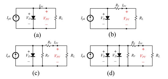
Figure 1.
Several PV models: (a) the ideal model, which is lossless; (b) single diode with series resistance; (c) single diode with series and parallel resistances; (d) the two-diode model.
The is the thermal voltage of the diode, which can be calculated by:
where n is called the ideality factor. The ideality factor indicates how close the diode is from the ideal diode. Therefore, if the diode is ideal. is the temperature of the cell in Kelvin, and is the Boltzmann constant, which has a value of . The amount of charge in one electron is C. The ideal model takes into account the direct relationship between the photocurrent and the solar insolation. However, it is not enough to model the nonideality, such as the losses. The simple model is similar to the ideal model with the addition of a series resistance , as shown in Figure 1b. The series resistance represents the losses in the low-doped semiconductor material, as well as the conduction losses in wires and contacts. The PV current is calculated by:
The series resistance is not enough to accurately model all the losses. The PV cell suffers from the impurities of the p-n junction and the leakage current across the cell borders, which lead to power loss. Therefore, parallel resistances model the loss and improve the temperature sensitivity. Figure 1c shows the equivalent circuit of the PV cell with the parallel resistance. The current equation of a single diode model with series and parallel resistance is given by:
A higher level of modeling accuracy can be achieved using the two-diode model, as shown in Figure 1d. The second diode represents the junction recombination, which corrects the ideality factor at low voltages. The current of the two-diode model is given by:
Several studies also introduced a three-diode model [37]. The current of the third diode represents recombinations in the blemished regions and grain boundaries. The current equation is given by:
2.2. PV Performance
The performance of a PV cell is related to its characteristic and power curves. The characteristic curve is also called the I-V curve, which shows the relationship between the PV voltage and current under specific solar irradiance and temperature, as shown in Figure 2a. Several parameters are known from the I-V curve, such as the open-circuit voltage, the short-circuit current, the voltage and current at the maximum power, and the maximum power point. Furthermore, the fill factor can be calculated, and it is given by:
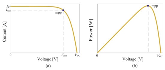
Figure 2.
The performance curves of PV cells: (a) I-V characteristic curve. From this curve, one can find the short-circuit current, open-circuit voltage, voltage and current at maximum power, fill factor, and resistance at maximum power. (b) P-V curve, which shows the maximum output power.
The performance also can be indicated using a power curve (P-V) that shows the power versus the voltage. Figure 2b shows the power curve under standard conditions. Under normal operation, the curve has a single peak, which represents the maximum power point. The irradiance level and temperature influence both the I-V and P-V curves. The effect of temperature on the P-V curve is illustrated in Figure 3a. As the temperature increases, the maximum output power decreases. On the other hand, the effect of irradiance on the PV curve is shown in Figure 3b. As the solar irradiance increases, the maximum power increases. Similarly, with the I-V curve, the increase in temperature reduces the open-circuit voltage, as shown in Figure 4. The short-circuit current increases as the solar irradiance increases. The effects of temperature on the open-circuit voltage and short-circuit current are given by:
where and the temperature coefficients for open-circuit voltage and the short-circuit current, respectively. The temperature of the standard test conditions (STCs) is given by . The open-circuit voltage and short-circuit current are measured in the STCs. The effect of solar irradiation on the short-circuit current can be characterized by:
where is the solar irradiation of the STCs, which is 1000 W/m:
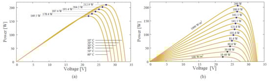
Figure 3.
The P-V under variable conditions: (a) Under different temperature degrees. (b) Under different solar irradiance levels.
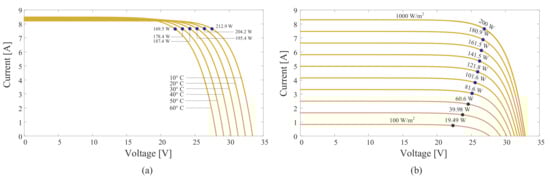
Figure 4.
The I-V under variable conditions: (a) Under different temperature degrees. (b) Under different solar irradiance levels.
3. Maximum Power Point Tracking Approaches
A single PV cell has a unique mpp, corresponding to the solar irradiance and temperature point. The resistance at that point is represented by . The at the STCs can be calculated by:
The variation in solar irradiance and temperature values makes variable. Therefore, a tracker is needed to allow a PV panel to operate at and extract the maximum power. Many approaches have been introduced to track the MPP. The commonly used technique in the solar industry is the P&O because of the reasonable trade-off between simplicity and performance. The P&O approach flowchart is seen in Figure 5. This approach perturbs the duty cycle and observes the power if it increases or decreases. Then, a step-change to the duty cycle takes place. The step-change determines the conversion speed and accuracy. P&O with a large step-change lacks accuracy and might experience instability issues. Making the step-change small reduces the conversion speeds, lacks speed, and might perform poorly at fast transitioning solar irradiance. The adaptive step can be applied, but without the guarantee of stable operation [36,38,39,40]. Similarly, hill-climbing and incremental conductance have similar performance to P&O, with no significant advantages. The ripple correlation control approach takes advantage of ripples imposed by switching devices on the PV panel [41,42]. In RCC, the derivative of the voltage is multiplied by the derivative of the power. If the product is zero, then the PV operates at its maximum power point. If the product is higher or lower than the MPP, then the PV operates on the left or the right of the MPP, respectively. The drawback of using RCC is the required multiplied devices, which are power-consuming devices.
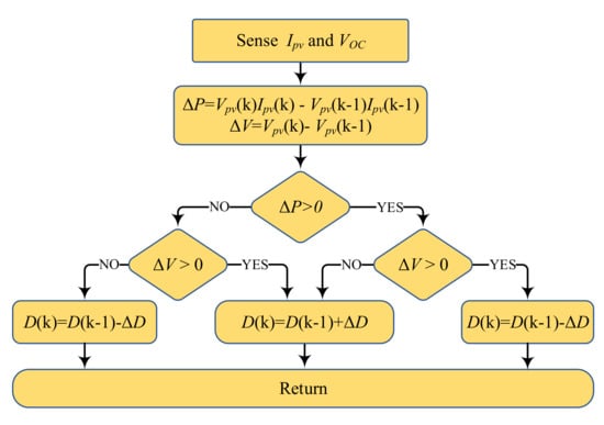
Figure 5.
The flowchart of the P&O tracking method.
Intelligent tracking approaches, such as fuzzy logic and artificial neural networks, were used to track the MPP. In fuzzy logic, the PV voltage and current are used to calculate the slope of the P-I characteristic and the change in the slope, which will be the input of the fuzzification stage. Fuzzification converts the numeric to linguistic variables to be used in the inference stage to make a decision. After a decision is made by a set of conditionals statements, the defuzzification stage converts the decision into numerical values [43,44,45]. Although the performance of the fuzzy controller is higher than the traditional P&O, the rules of the membership function selection are based on trial and error, which increases the implementation time. The neural network method was used to track the MPP. The technique uses acquired data, usually irradiance and temperature, to train the neurons and provide the optimal weight that makes the correct control decision about the duty [46,47]. The NN can track the true MPP and has solid performance, but it uses an expensive pyranometer to read the irradiance values.
The fractional open-circuit voltage (FOCV) method is the simplest MPPT method. In this method, the MPP voltage can be approximated by multiplying the open-circuit voltage with a fraction number k. The k is a constant value predetermined by either experimentation or assumption, and it has a typical value ranging between and . The open-circuit voltage must be sensed periodically. The challenge is that the open-circuit voltage cannot be measured while the system operates without disconnecting the system. Disconnecting the system momentarily to measure the open-circuit voltage leads to power loss and overall efficiency degradation. In order to find the open-circuit voltage without PV panel disconnection, a pilot cell with the same characteristics as the main PV panel is needed. Figure 6 shows the implementation of the FOCV with a pilot cell.
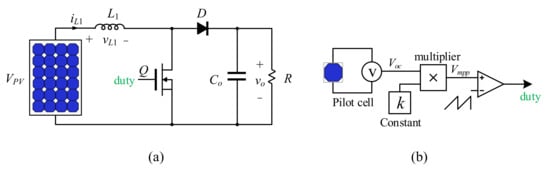
Figure 6.
An example of how FOCV with the pilot cell is implemented: (a) the PV is connected to a conventional boost converter, which is controlled by the duty cycle (b) the pilot cell provides the reading of the to the control circuit.
4. The Proposed Method
4.1. Theory of Operation
The conventional FOCV is unable to reach the actual MPP, and neural network methods require expensive sensors to give accurate results. The proposed method uses a neural network to correlate the open-circuit voltage with temperature, therefore giving the right and precise reference voltage or duty cycle. The proposed FFNN is fed input from an external pilot circuit and a temperature sensor. The external pilot cell provides implicit information about the solar irradiance level and independent open-circuit voltage without system disconnection. Figure 7a shows the maximum power of the PV plotted versus the voltage and current of the PV panel. We use a neural network to learn and approximate maximum power functions perfectly under specific solar irradiance and temperature. Therefore, the reading of the irradiance and temperature is needed to find the real MPP. The ratio between the maximum power voltage and the open-circuit voltage varies depending on the irradiance level and the temperature, as shown in Figure 7b. The PV panel’s open-circuit voltage directly relates to the irradiance and an inverse relationship with the temperature, as illustrated in Figure 7c. Similarly, the effects of solar irradiance and temperature on the maximum power and the relationship between the maximum power and maximum voltage and current are shown in Figure 7d and Figure 7e, respectively. The figures show that the open-circuit voltage can provide information about the solar irradiance, and by using only the temperature sensor, the true MPPs can be found.
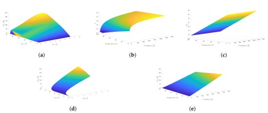
Figure 7.
(a) The output power of the PV panel versus the PV current and PV voltage. (b) The ratio
between the maximum voltage versus the irradiance and temperature. (c) The effects of solar irradiance and temperature on the open-circuit voltage of the PV panel. (d) The effects of solar irradiance and temperature on the maximum power of the PV panel. (e) The maximum power versus the maximum
current and the maximum voltage of the PV.
4.2. Neural Network Based FOCV Setup
The setup has three stages; preprocessing, setting and training the neural network, and implementation and testing. Figure 8 shows the stages of implementing the controller.
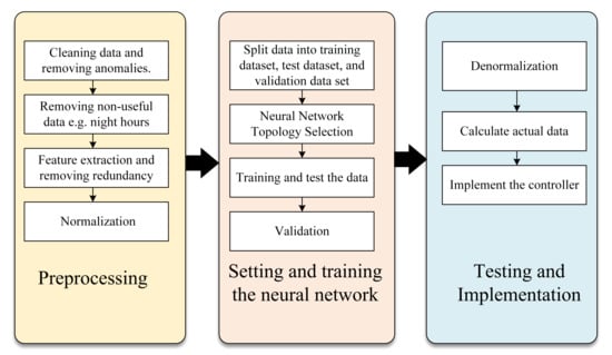
Figure 8.
Stages for implementing the neural network based FOC controller. The implementation process has three stages; preprocessing, setting and training the neural network, and testing and implementation.
4.2.1. Preprocessing
The data can be obtained using voltage sweep at different solar irradiance, either experimentally or by simulation. Figure 9 shows the circuit used to obtain the dataset, which can be either simulation or experimental. A large dataset is needed to train the network and achieve higher test accuracy. The process can be automated in simulation using an iterative loop with a small step size, which allows for higher resolution data. The data obtained must be correctly labeled. Each maximum power point and open-circuit voltage correspond to specific solar irradiance and temperature values. In this study, the Kyocera KC200GT solar panel was used to perform the sweep. The panel was tested at standard test conditions (STCs), which had 200 W maximum power, V, A, V, and A. The data were recorded in the solar irradiance range of 50−1000 W/m and temperature range of 15−65 C. The recorded data require cleaning the incorrect sensor readings or other values that are out of PV range, for example negative values of power. Missing data points can be filled with the average of the row or the mode. Because the data are obtained by the voltage sweep, some data are redundant. The redundancy needs to be removed to improve the training process. Table 1 shows a sample of the recorded data after cleaning. The final step in the preprocessing stage is normalization. Normalization enhances the learning speed and convergence time [48]. The values after the normalization process lie between 0 and 1.
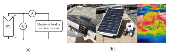
Figure 9.
The approach used to produce the dataset for neural network training: (a) schematic diagram of the circuit (b) experimental setup. The electronic load used to sweep the voltage and get the I-V characteristic curve at specific irradiance and temperature values.

Table 1.
Sample of the recorded data.
4.2.2. Setting the Network And Training
In this stage, the data are split into a training dataset and a testing dataset, either by using a holdout set or a cross-validation set. The validation dataset is optional, and the controller can be validated eventually after simulation and implementation. The holdout set used is 70% for training and 30% for the test. The selection of the neural network topology can be difficult due to the wide variety of neural network topologies and hyperparameters. A feedforward neural network is used in this paper to map labeled input data to labeled output data and learn the relationship. Figure 10 shows the structure of the training network. The training consists of two neural networks. The first neural network is used to approximate the relationship between the open-circuit voltage and the solar irradiance under variable temperature values. eliminates the need for an expensive pyranometer, as the solar irradiance can be estimated with the value of open-circuit voltage. The structure of contains an input layer with two neurons, a hidden layer with 8 neurons, and a single output layer. The activation function of the hidden layer is [49], which is given by:
where z is nothing but the summation of the bias and the product of the weight and input examples . The output layer has a linear function where . The inputs to are and the temperature , and the target is the solar irradiance . Similarly, has an input layer that takes two inputs, the predicted irradiance and the temperature . The hidden layer consists of 10 neurons with the activation function. The output layer has a linear activation function, and the output is k.
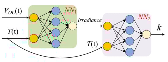
Figure 10.
The two neural networks used in training: used to approximate the relationship between the open-circuit voltage and the solar irradiance under variable temperature values, and used to map the relationship between the irradiance and fractional open-circuit factor.
After selecting the topology, the weight is randomized, and the hyperparameters are set. Both networks are trained using the Levenberg–Marquardt backpropagation algorithm [50] to update the weight. The training took about 50 epochs to reach the goal set, a low mean squared error (MSE).
4.2.3. Testing and Implementation of The Controller
After the training process is complete, the weight and bias are adjusted to map the relationship between the inputs and the output correctly. Then, the data are denormalized; the reverse of the normalization process. To evaluate the performance of the neural network, the mean squared error is used, which is given by:
where is the predicted output value and n is the number of samples. The learning curve of the training process and testing is shown in Figure 11. The MSE error is about at the end of the 50th epoch. The neural network block is implemented using the following equation.
where are the weight matrix for the hidden layer, the weight matrix for the output layer, the bias for the hidden layer, and the output layer’s bias, respectively. A multiplier is then used to find the voltage reference by multiplying the open-circuit voltage and the fraction k. A further safe operation can be considered by limiting the value of k to be between 0 and 1.
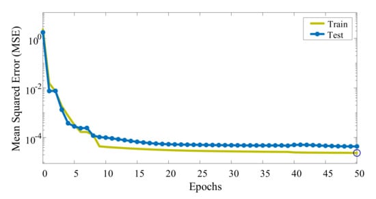
Figure 11.
The learning curve for training . The performance of the test is similar to the training.
5. Simulations
The simulation setup of the proposed method was implemented using MATLAB and PLECS Blockset, as shown in Figure 12. The model KC200GT was used as an input source to supply a resistive load. The PV system was interfaced using a Ćuk converter, as shown in Figure 12a. The Ćuk converter was selected because of the non-pulsating input and output currents, which enhance the PV cell’s lifetime and obtain better reading values of the PV current, as well as providing the ability to step-up and step-down the voltage. Then, the resistance of the maximum power point (Rmpp) can be tracked from zero to infinity ∞. The Ćuk converter is designed to operate in continuous conduction mode, where the inductor current at the input level must be above zero in the steady-state. In the continuous conduction mode, the converter goes into two subintervals. In Subinterval 1, the MOSFET is ON, and the diode is in reverse bias mode. The inductor is charging from the input source, and the capacitor is discharging to the output. The equivalent circuit of this subinterval is illustrated in Figure 13a. In Subinterval 2, the MOSFET is OFF, and the diode is in forwarding conduction mode. The capacitor is charging from the input source and the inductor . The equivalent circuit of Subinterval 2 is shown in Figure 13b. The output voltage of the Ćuk converter is inverted and given by:
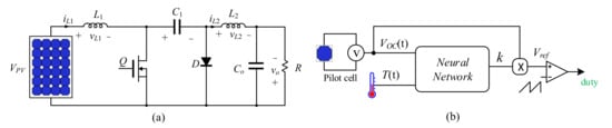
Figure 12.
The experimental setup: (a) Ćuk converter (b) the proposed controller.
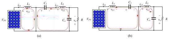
Figure 13.
The subintervals in continuous conduction mode. (a) is when the active switch is ON; (b) is the when the active switch is OFF.
The parameters used in the simulation are H, H, F, V, m. The MPPT tracker shown in Figure 12b consists of the pilot PV cell and the neural network. The pilot PV cell is connected directly to a voltage sensor to obtain the open-circuit voltage. The controller uses a pilot cell for open-circuit voltage measurements and a temperature sensor to provide temperature values. Then, the trained neural network takes the and values at time t and provides the corresponding k. The value of k will be multiplied by to provide the reference voltage to the pulse width modulator (PWM). The PWM operates at a 100 kHz switching frequency, and the control bandwidth does not exceed one-tenth of the switching frequency.
5.1. Case1: Variation of Solar Irradiance with a Constant Temperature Value
In this case, the output load and temperature are assumed constant for two reasons. First, the relationship between the output power and solar irradiance is stronger than the relationship between the output load and temperature, which gives an acceptable estimation of the tracking algorithm’s performance if the temperature value is constant. Second, all algorithms need an ideal test, where the load is constant to find their best performance. Figure 14 shows the performance of the algorithms under the variation of solar irradiance. The proposed method outperforms the P&O algorithm in terms of accuracy and can reach the MPP faster. P&O oscillates around the MPP without reaching the exact MPP. The FOCV method has a similar dynamic performance to the proposed method. However, the accuracy of the FOCV is less than the proposed method.
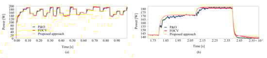
Figure 14.
The output waveform of the PV panel for Case 1 using various tracking algorithm: (a) The performance over a long time period. (b) Zoomed area.
Figure 15 shows a new way to compare the performance of the two algorithms. Therefore in Figure 15a, the power difference between the FOCV and the proposed method is shown to indicated positive and negative regions. The positive region is when the difference in power is higher than zero, which indicates that the power produced using the proposed method is higher than the power produced using the FOCV. The negative region is when the difference in power is less than zero and indicates that the FOCV performs better. The comparison with P&O is shown in Figure 15b.
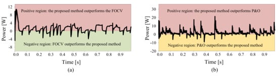
Figure 15.
Case 1: comparison between the proposed method with (a) the FOCV method and (b) the P&O method.
5.2. Variation of Both Irradiance and Temperature
This case simulates a more realistic situation, where the temperature and irradiance vary. The output power, in this case, is shown in Figure 16. It can be seen that the proposed method exhibits faster dynamic speed and higher accuracy than the other methods. The varying temperature greatly degrades the performance of the FOCV since the open-circuit voltage depends on it. P&O is also affected by the temperature variation. However, since the P&O algorithm is independent of the panel information, the accuracy is higher than the FOCV method. The proposed method is faster during transitions from one irradiance level to another.
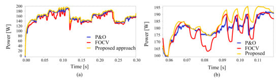
Figure 16.
The output waveform of the PV panel for Case 2 using various tracking algorithms: (a) The performance over a long time period. (b) Zoomed area.
5.3. Energy Analysis
It can be seen from Figure 14, Figure 15, Figure 16 and Figure 17 that the proposed converter outperforms the other tracking algorithms. The overall comparison can be determined using the average of the difference between the two tracking methods. In the case of fixed temperature, the extracted energy by the proposed method is about 4.27 kW/y higher than the FOCV and 5.1 kWh/y higher than P&O. In the case of variable temperature, the energy extracted by the proposed method is 12.1 kWh/y higher than the extracted energy by the FOCV and 8.9 kWh/y higher than the extracted energy by P&O. Note that the previous analysis is per panel; the difference in energy extraction would be much higher for a large PV system. The performance comparison is summarized in Table 2. The energy and efficiency of the proposed are higher than the other methods, with better transitioning time and stability.
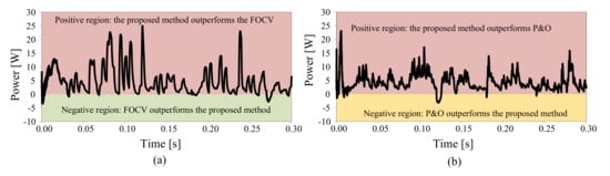
Figure 17.
Case 2: comparison between the proposed method with (a) the FOCV method and (b) the P&O method.
Table 2.
Performance comparison of the proposed method with commonly used methods.
6. Conclusions
A novel approach for finding the maximum power point of a photovoltaic system is developed. The approach is based on the fractional open-circuit voltage to find the true maximum power point using an artificial neural network approach. The neural network can correlate the reference voltage of the maximum power to the open-circuit voltage and temperature. Unlike other neural network approaches, the presented approach does not require expensive irradiance sensor circuitry. The proposed method is used to control the Ćuk converter to interface with a 200 W solar panel. Both the simulation and experimental results confirm the validation of the new approach. The results show that the proposed method has a fast transitioning time, better efficiency, and higher extracted energy than other methods.
Funding
This research was funded by Najran University Grant Number NU/ESCI/17/075.
Acknowledgments
The author is thankful to the Deanship of Scientific Research at Najran University for funding this work through Grant Research Code NU/ESCI/17/075.
Conflicts of Interest
The author declares no conflict of interest.
Abbreviations
The following abbreviations are used in this manuscript:
| PV | Photovoltaics |
| MPPT | Maximum power point tracking |
| FFNN | Feedforward neural network |
| FOCV | Fractional circuit voltage |
References
- Fayaz, H.; Rahim, N.; Saidur, R.; Solangi, K.; Niaz, H.; Hossain, M. Solar energy policy: Malaysia vs developed countries. In Proceedings of the 2011 IEEE Conference on Clean Energy and Technology (CET), Kuala Lumpur, Malaysia, 27–29 June 2011; pp. 374–378. [Google Scholar]
- Mendoza, J.M.F.; Gallego-Schmid, A.; Rivera, X.C.S.; Rieradevall, J.; Azapagic, A. Sustainability assessment of home-made solar cookers for use in developed countries. Sci. Total Environ. 2019, 648, 184–196. [Google Scholar] [CrossRef] [PubMed]
- Liu, Z. What is the future of solar energy? Economic and policy barriers. Energy Sources Part Econ. Planning Policy 2018, 13, 169–172. [Google Scholar] [CrossRef]
- Irfan, M.; Zhao, Z.Y.; Ikram, M.; Gilal, N.G.; Li, H.; Rehman, A. Assessment of India’s energy dynamics: Prospects of solar energy. J. Renew. Sustain. Energy 2020, 12, 053701. [Google Scholar] [CrossRef]
- Messenger, R.A.; Abtahi, A. Photovoltaic Systems Engineering; CRC Press: Boca Raton, FL, USA, 2017. [Google Scholar]
- Tyagi, V.; Rahim, N.A.; Rahim, N.; Jeyraj, A.; Selvaraj, L. Progress in solar PV technology: Research and achievement. Renew. Sustain. Energy Rev. 2013, 20, 443–461. [Google Scholar] [CrossRef]
- Villalva, M.G.; Gazoli, J.R.; Ruppert Filho, E. Comprehensive approach to modeling and simulation of photovoltaic arrays. IEEE Trans. Power Electron. 2009, 24, 1198–1208. [Google Scholar] [CrossRef]
- Shi, Y.; Li, R.; Xue, Y.; Li, H. High-frequency-link-based grid-tied PV system with small DC-link capacitor and low-frequency ripple-free maximum power point tracking. IEEE Trans. Power Electron. 2015, 31, 328–339. [Google Scholar] [CrossRef]
- Ghenai, C.; Bettayeb, M. Design and optimization of grid-tied and off-grid solar PV systems for super-efficient electrical appliances. Energy Effic. 2020, 13, 291–305. [Google Scholar] [CrossRef]
- Rafique, M.M.; Bahaidarah, H.M.; Anwar, M.K. Enabling private sector investment in off-grid electrification for cleaner production: Optimum designing and achievable rate of unit electricity. J. Clean. Prod. 2019, 206, 508–523. [Google Scholar] [CrossRef]
- Kavya Santhoshi, B.; Mohana Sundaram, K.; Padmanaban, S.; Holm-Nielsen, J.B.; KK, P. Critical review of PV grid-tied inverters. Energies 2019, 12, 1921. [Google Scholar] [CrossRef]
- Qing, X.; Niu, Y. Hourly day-ahead solar irradiance prediction using weather forecasts by LSTM. Energy 2018, 148, 461–468. [Google Scholar] [CrossRef]
- Khosravi, A.; Koury, R.; Machado, L.; Pabon, J. Prediction of hourly solar radiation in Abu Musa Island using machine learning algorithms. J. Clean. Prod. 2018, 176, 63–75. [Google Scholar] [CrossRef]
- Dong, N.; Chang, J.F.; Wu, A.G.; Gao, Z.K. A novel convolutional neural network framework based solar irradiance prediction method. Int. J. Electr. Power Energy Syst. 2020, 114, 105411. [Google Scholar] [CrossRef]
- Esram, T.; Chapman, P. Comparision of Photovoltaic Array MPPT Techniques. IEEE Trans. Energy Convers. 2007, 22, 439–449. [Google Scholar] [CrossRef]
- Liu, F.; Duan, S.; Liu, F.; Liu, B.; Kang, Y. A variable step size INC MPPT method for PV systems. IEEE Trans. Ind. Electron. 2008, 55, 2622–2628. [Google Scholar]
- Subudhi, B.; Pradhan, R. A comparative study on maximum power point tracking techniques for photovoltaic power systems. IEEE Trans. Sustain. Energy 2012, 4, 89–98. [Google Scholar] [CrossRef]
- Abdelsalam, A.K.; Massoud, A.M.; Ahmed, S.; Enjeti, P.N. High-performance adaptive perturb and observe MPPT technique for photovoltaic-based microgrids. IEEE Trans. Power Electron. 2011, 26, 1010–1021. [Google Scholar] [CrossRef]
- Mei, Q.; Shan, M.; Liu, L.; Guerrero, J.M. A novel improved variable step-size incremental-resistance MPPT method for PV systems. IEEE Trans. Ind. Electron. 2010, 58, 2427–2434. [Google Scholar] [CrossRef]
- Lin, L.; Zhang, J.; Shao, S. Differential Power Processing Architecture With Virtual Port Connected in Series and MPPT in Submodule Level. IEEE Access 2020, 8, 137897–137909. [Google Scholar] [CrossRef]
- Motahhir, S.; El Hammoumi, A.; El Ghzizal, A. The most used MPPT algorithms: Review and the suitable low-cost embedded board for each algorithm. J. Clean. Prod. 2020, 246, 118983. [Google Scholar] [CrossRef]
- Bollipo, R.B.; Mikkili, S.; Bonthagorla, P.K. Critical Review on PV MPPT Techniques: Classical, Intelligent and Optimisation. IET Renew. Power Gener. 2020, 14, 1433–1452. [Google Scholar]
- Pathak, P.K.; Yadav, A.K.; Alvi, P. Advanced Solar MPPT Techniques Under Uniform and Non-Uniform Irradiance: A Comprehensive Review. J. Sol. Energy Eng. 2020, 142. [Google Scholar] [CrossRef]
- Mansoor, M.; Mirza, A.F.; Ling, Q. Harris hawk optimization-based MPPT control for PV Systems under Partial Shading Conditions. J. Clean. Prod. 2020, 274, 122857. [Google Scholar] [CrossRef]
- Abdel-Rahim, O.; Alamir, N.; Orabi, M.; Ismeil, M. Fixed-frequency phase-shift modulated PV-MPPT for LLC resonant converters. J. Power Electron. 2020, 20, 279–291. [Google Scholar] [CrossRef]
- Pradhan, R.; Panda, A. Performance evaluation of a MPPT controller with model predictive control for a photovoltaic system. Int. J. Electron. 2020, 107, 1543–1558. [Google Scholar] [CrossRef]
- De Brito, M.A.G.; Galotto, L.; Sampaio, L.P.; e Melo, G.d.A.; Canesin, C.A. Evaluation of the main MPPT techniques for photovoltaic applications. IEEE Trans. Ind. Electron. 2012, 60, 1156–1167. [Google Scholar] [CrossRef]
- Chen, W.; Shen, H.; Shu, B.; Qin, H.; Deng, T. Evaluation of performance of MPPT devices in PV systems with storage batteries. Renew. Energy 2007, 32, 1611–1622. [Google Scholar] [CrossRef]
- Uoya, M.; Koizumi, H. A calculation method of photovoltaic array’s operating point for MPPT evaluation based on one-dimensional Newton–Raphson method. IEEE Trans. Ind. Appl. 2014, 51, 567–575. [Google Scholar] [CrossRef]
- Rezk, H.; Mazen, A.O.; Gomaa, M.R.; Tolba, M.A.; Fathy, A.; Abdelkareem, M.A.; Olabi, A.; Abou Hashema, M. A novel statistical performance evaluation of most modern optimization-based global MPPT techniques for partially shaded PV system. Renew. Sustain. Energy Rev. 2019, 115, 109372. [Google Scholar] [CrossRef]
- Garcia, M.; Maruri, J.M.; Marroyo, L.; Lorenzo, E.; Pérez, M. Partial shadowing, MPPT performance and inverter configurations: Observations at tracking PV plants. Prog. Photovoltaics Res. Appl. 2008, 16, 529–536. [Google Scholar] [CrossRef]
- Femia, N.; Petrone, G.; Spagnuolo, G.; Vitelli, M. Optimization of perturb and observe maximum power point tracking method. IEEE Trans. Power Electron. 2005, 20, 963–973. [Google Scholar] [CrossRef]
- Hussein, K.; Muta, I.; Hoshino, T.; Osakada, M. Maximum photovoltaic power tracking: An algorithm for rapidly changing atmospheric conditions. IEE Proc. Gener. Transm. Distrib. 1995, 142, 59–64. [Google Scholar] [CrossRef]
- Salas, V.; Olias, E.; Barrado, A.; Lazaro, A. Review of the maximum power point tracking algorithms for stand-alone photovoltaic systems. Sol. Energy Mater. Sol. Cells 2006, 90, 1555–1578. [Google Scholar] [CrossRef]
- Elgendy, M.A.; Zahawi, B.; Atkinson, D.J. Assessment of perturb and observe MPPT algorithm implementation techniques for PV pumping applications. IEEE Trans. Sustain. Energy 2011, 3, 21–33. [Google Scholar] [CrossRef]
- Xiao, W.; Dunford, W.G. A modified adaptive hill climbing MPPT method for photovoltaic power systems. In Proceedings of the 2004 IEEE 35th Annual Power Electronics Specialists Conference (IEEE Cat. No. 04CH37551), Aachen, Germany, 20–25 June 2004; Volume 3, pp. 1957–1963. [Google Scholar]
- Nishioka, K.; Sakitani, N.; Uraoka, Y.; Fuyuki, T. Analysis of multicrystalline silicon solar cells by modified 3-diode equivalent circuit model taking leakage current through periphery into consideration. Sol. Energy Mater. Sol. Cells 2007, 91, 1222–1227. [Google Scholar] [CrossRef]
- Brunton, S.L.; Rowley, C.W.; Kulkarni, S.R.; Clarkson, C. Maximum power point tracking for photovoltaic optimization using ripple-based extremum seeking control. IEEE Trans. Power Electron. 2010, 25, 2531–2540. [Google Scholar] [CrossRef]
- Mohammad, A.N.M.; Radzi, M.A.M.; Azis, N.; Shafie, S.; Zainuri, M.A.A.M. An Enhanced Adaptive Perturb and Observe Technique for Efficient Maximum Power Point Tracking Under Partial Shading Conditions. Appl. Sci. 2020, 10, 3912. [Google Scholar] [CrossRef]
- Liu, F.; Kang, Y.; Zhang, Y.; Duan, S. Comparison of P&O and hill climbing MPPT methods for grid-connected PV converter. In Proceedings of the 2008 3rd IEEE Conference on Industrial Electronics and Applications, Singapore, 3–5 June 2008; pp. 804–807. [Google Scholar]
- Esram, T.; Kimball, J.W.; Krein, P.T.; Chapman, P.L.; Midya, P. Dynamic maximum power point tracking of photovoltaic arrays using ripple correlation control. IEEE Trans. Power Electron. 2006, 21, 1282–1291. [Google Scholar] [CrossRef]
- Hammami, M.; Grandi, G. A single-phase multilevel PV generation system with an improved ripple correlation control MPPT algorithm. Energies 2017, 10, 2037. [Google Scholar] [CrossRef]
- Kottas, T.L.; Boutalis, Y.S.; Karlis, A.D. New maximum power point tracker for PV arrays using fuzzy controller in close cooperation with fuzzy cognitive networks. IEEE Trans. Energy Convers. 2006, 21, 793–803. [Google Scholar] [CrossRef]
- Alajmi, B.N.; Ahmed, K.H.; Finney, S.J.; Williams, B.W. Fuzzy-logic-control approach of a modified hill-climbing method for maximum power point in microgrid standalone photovoltaic system. IEEE Trans. Power Electron. 2010, 26, 1022–1030. [Google Scholar] [CrossRef]
- Bendib, B.; Krim, F.; Belmili, H.; Almi, M.; Boulouma, S. Advanced Fuzzy MPPT Controller for a stand-alone PV system. Energy Procedia 2014, 50, 383–392. [Google Scholar] [CrossRef]
- Lin, W.M.; Hong, C.M.; Chen, C.H. Neural-network-based MPPT control of a stand-alone hybrid power generation system. IEEE Trans. Power Electron. 2011, 26, 3571–3581. [Google Scholar] [CrossRef]
- Zečević, Ž.; Rolevski, M. Neural Network Approach to MPPT Control and Irradiance Estimation. Appl. Sci. 2020, 10, 5051. [Google Scholar] [CrossRef]
- Mueller, A.V.; Hemond, H.F. Extended artificial neural networks: Incorporation of a priori chemical knowledge enables use of ion selective electrodes for in-situ measurement of ions at environmentally relevant levels. Talanta 2013, 117, 112–118. [Google Scholar] [CrossRef] [PubMed]
- Simpson, P.K. Artificial Neural Systems: Foundations, Paradigms, Applications, and Implementations; Elsevier Science Inc.: Amsterdam, The Netherlands, 1989. [Google Scholar]
- Hagan, M.T.; Menhaj, M.B. Training feedforward networks with the Marquardt algorithm. IEEE Trans. Neural Netw. 1994, 5, 989–993. [Google Scholar] [CrossRef] [PubMed]


Publisher’s Note: MDPI stays neutral with regard to jurisdictional claims in published maps and institutional affiliations. |
© 2020 by the author. Licensee MDPI, Basel, Switzerland. This article is an open access article distributed under the terms and conditions of the Creative Commons Attribution (CC BY) license (http://creativecommons.org/licenses/by/4.0/).