Sensing Occupancy through Software: Smart Parking Proof of Concept

Abstract

In order to detect the vehicle presence in parking slots, different approaches have been utilized, which range from image recognition to sensing via detection nodes. The last one is usually based on getting the presence data from one or more sensors (commonly magnetic or IR-based), controlled and processed by a micro-controller that sends the data through radio interface. Consequently, given nodes have multiple components, adequate software is required for its control and state-machine to communicate its status to the receiver. This paper presents an alternative, cost-effective beacon-based mechanism for sensing the vehicle presence. It is based on the well-known effect that, once the metallic obstacle (i.e., vehicle) is on top of the sensing node, the signal strength will be attenuated, while the same shall be recognized at the receiver side. Therefore, the signal strength change conveys the information regarding the presence. Algorithms processing signal strength change at the receiver side to estimate the presence are required due to the stochastic nature of signal strength parameters. In order to prove the concept, experimental setup based on LoRa-based parking sensors was used to gather occupancy/signal strength data. In order to extract the information of presence, the Hidden Markov Model (HMM) was employed with accuracy of up to 96%, while the Neural Network (NN) approach reaches an accuracy of up to 97%. The given approach reduces the costs of the sensor production by at least 50%.

1. Introduction

Intense technological development currently is reshaping many areas of everyday life and impacting human behavior. The Internet of Things (IoT) vision of ubiquitous and pervasive connection of smart things gives rise to a future environment that is composed out of physical and digital world. In this environment, it is possible to receive information about or from the psychical world that was previously not available to us and, moreover, interconnect it to exchange and use this information with the digital world [1]. The IoT applications are being employed in diverse areas of industry, communication, wireless sensor networks, data mining, assisted living, etc., giving rise to the concept of Smart City.

The Smart City is constituted out of gathered and processed information, covering a wide range of entities, such as transportation, health, food, and education for the overall improvement of life quality [2]. One of the most important topics addressed by the European Commission and most nations in the world is the development of an urban city model that aimed at increasing the quality of life of people working and living in them. Smart and Sustainable Mobility is one of the central concepts in the vision of the Smart City, where IoT plays an important role [3,4]. In urban city areas, due to the rise of cars, existing parking systems are inadequate or unable to handle parking loads [5]. Moreover, parking facilities are not accessible in a adequate manner, since it is estimated that drivers spend around 7.8 min. in finding free parking lots [6]. Studies have shown that, in traffic dens environments in urban areas, 30–50% of drivers are in search of free parking [7]. In addition, the IBM survey (IBM Survey. Available online: https://www-03.ibm.com/press/us/en/pressrelease/35515.wss (accessed on 20 November 2020)) reported that due to traffic in metropolitan cities such as Beijing or Madrid drivers spend, on average, 30 to 40 min. searching a free parking space. The increase of fuel consumption and air pollution is one of the major issues that arise from this [8]. Furthermore, the consequences of traffic jams are the frustration of drivers and higher probability of accidents [7]. Finally, traffic congestion leads to cost-effective losses, since, in a city of 50,000 inhabitants, having, on average, 250 parking lots, generates an annual cost of 216,000 US dollars [9].

In the last decade, the development of dynamic and complex IoT system and number of connected devices keeps increasing exponentially as well as the data that were collected by these devices that need to be properly analyzed [10]. Effective analysis of big data can extract meaningful information and correlation amongst vast quantities of data that are generated by sensor devices, which are a key factor in the success in many domains and, especially, in the Smart City applications [11]. Therefore, IoT devices need to be able to manage data collection, Machine-to-Machine (M2M) communication, pre-processing of the data if needed, whilst compensating among cost, processing power, and energy consumption [12].

Along with great advancements in technology, including the availability of cheap and massive computing, hardware and storage arose Machine Learning (ML) holding a vast potential for data analysis, and precise predictions made from the past observations for given new measurements [13]. Machine learning is the most prominent artificial intelligence (AI) algorithm, which has been utilized in various fields from computer vision, computer graphics, natural language processing (NLP) to speech recognition, decision-making, and intelligent control [14], as well as in intrusion detection systems [15]. Within IoT devices, the application of ML can enable users to gain deeper insight into data correlations and mine the information and features that are hidden within this data [16]. With that regard, IoT applications that use sensor technology, RFID technology, network communication, data mining and machine learning could prove to be quite efficient in solving the previously presented problem of free parking space [17].

Deep Learning methods, such as deep long short term memory network (LSTM), have been recently applied for the prediction of available free parking space [18]. A recent review of literature presented in [19] pointed to several open issues and challenges with regards to the design of Smart Parking spaces, emphasizing the utilization of car parking with emerging technologies, such as Deep Learning. A commonly and widely used model for sequential or time series data in ML and statistics is the Hidden Markov Model (HMM) [20]. HMMs are based on the concept of Markov Chain, and they can represent any random sequential process that undergoes transitions from one state to another [21]. In the last two decades, HMM has been used in various areas as a data-driven modeling approach in automatic speech recognition, pattern recognition, signal processing, telecommunication, bioinformatics, etc. [22]. Recent works of researches incorporated Markov models for parking space occupancy predictions. For instance, in [23], the authors propose a model-based framework in order to predict future occupancy from historical occupancy data. The foundation of this predictive framework is continuous-time Markov queuing model, which is employed to describe the stochastic occupancy change of a parking facility. The model was evaluated while using a mean absolute relative error (MARE), ranging from 5.23% to 1.86% for different case studies. Furthermore, in [24], an agent-based service combined with a learning and prediction system that uses a time varying Markov chain to predict parking availability is proposed. Agents predict the parking availability in a given parking garage and communicate with other agents in order to produce a cumulative prediction achieving prediction accuracy of about 83%.

In recent years, the field of Deep Learning has become rather prominent, and the concept of artificial Neural Networks (NN), which are inspired by brain nervous system, has gained significant interest amongst researches [25]. Neural Networks have the capacity to learn hierarchical representations and are well suited for machine perception tasks, where the crude underlying features cannot be individually interpreted [26]. This makes them a powerful ML tool that achieves state-of-the-art results in a wide range of supervised and unsupervised machine learning tasks. Neural Networks have been efficiently implemented in a variety of fields like patter recognition, signal processing and control of complex nonlinear systems [25]. Moreover, NNs have also been applied in prediction of future occupancy status such as in [27,28]. Using the data regarding the duration of free parking space and occupancy status, the researches in [27] have developed a short-term and long term parking availability prediction system based on Neural Network. They have concluded that NNs can adequately capture the temporal transformations of parking status providing accurate prediction of occupancy up to half an hour ahead. More recently, in [28], the authors use a Deep Learning Neural Network for parking lot occupancy status classification that is based on a images of parking spaces, giving 93% correct classification rate for a particular data set.

Existing Smart Parking solutions for detecting occupancy include the usage of adequate sensing technologies and transmission to a centralized system for further processing (using appropriate radio technology, such as LoRa, NB-IoT, Sigfox, BLE5, etc.). Such devices use detection techniques that are based on sensors, such as light, magnetometer, infrared detector, distance sensors, or a combination of sensing technologies [29,30,31,32]. Moreover, the researchers in [33] point out that the employment of a purposeful Smart Parking solution must take into account people with special needs and enable parking for disabled. Therefore, they have utilized RFID and database authentication for the use of ultrasonic sensors, LED, and cloud technology method for better and improved disabled parking management. However, these solutions are rather power hungry, due to the consumption of a large number of sensors, microcontrollers (MCUs), and radio communication peripherals, which impact the lifetime of an otherwise battery-powered device. Consequently, the existence of sensing technologies in Smart Parking sensor devices often requires from manufacturer the implementation of circuitry that requires, from MCU, a state-machine capable methodology, adequate software for sensor activation and sensor readings, and decision making about, and radio communication upon, parking status changes. In addition, such devices are usually implemented with the capability to receive communication over the radio from centralized systems/gateways for making updates (e.g., duty cycle period, time synchronization), but also perform online firmware updates. Taking into account additional requirements from the end user to calibrate sensors prior installing them, there is a need for an alternative solution that would be easier to implement. The research that is presented in this paper proposes a hardware sensing solution through software that uses signal strength information to achieve cost savings. A novel software approach would employ appropriate ML algorithms to gain a high level of occupancy status detection, thus achieving cost saving by reducing the price of the sensing device. The idea of such a solution has found its basis in some recent research that observed a scenario in which the signal strength at the receiver side is significantly reduced [6,34] when a vehicle occupies a parking lot. Emerging techniques, like Machine Learning and intelligent sensing in car parks, might be able to efficiently reduce the parking search time and improve mobility [19]. Similarly, it has been observed that the measurement of the received signal strength from the LoRa radio module could serve as a humidity indicator for the purpose of soil moisture detection [35,36]. In the parking environment, when something changes, such as when the car goes over the sensor device covering the parking lot, signal strength at the receiver side will change. This indicates that the signal strength change also holds information about the vehicle presence. Using the above principle in which the vehicle presence can cause a drop in signal power at the receiver side from a LoRa-based device, this paper introduces a novel system for the cost-effective and low-power detection of parking slot occupancy. Because signal strength change and parking occupancy present highly correlated processes, it is reasonable to use machine learning techniques, such as Hidden Markov Model and Neural Networks, for detecting/estimating occupancy from signal strength change with a low error rate. This way, the hardware problem of sensing occupancy is solved through software while using HMM and NN, where a high estimation detection result is achieved, which, at the end, will result in reducing the overall price of the sensing device. Consequently, the device will become a simple beacon device (without any sensor), where occupancy is detected with a significant change in signal strength. Moreover, the proposed solution could also serve as additional sensor to already existing parking lot detection techniques in order to improve parking lot occupancy monitoring, without any hardware changes to existing sensing techniques. Using techniques that are based on the Hidden Markov Model, it is possible to estimate parking space occupancy based on signal strength with an accuracy of up to 96%. When introducing machine learning techniques that are based on Neural Networks, parking lot occupancy can be correctly estimated with an accuracy of up to 97%.

2. State of the Art

Smart Parking solutions vary with regards to sensing technologies and methods that are used for parking space occupancy prediction and classification. When regarding the architecture of these solution it can be noticed that it is generally constituted out of three distinguishing components: type of sensors, network protocols, and software solutions [37]. In [38], the authors designed a prototype of a parking occupancy monitoring and visualization system that uses an ultrasonic sensor being controlled by an Arduino Uno which uses a Wireless XBee shield and an XBee Series 2 module for communication. The data collected from the sensor is then given as an input to a algorithm that detects parking space statues and reports to a database in a real-time basis. Moreover, in [39], the authors presented a novel system for detecting the cruising behavior in vehicle journeys and developed a real-time parking information system. The system uses GPS sensors as an application that sends the user’s location and allows for the system to create a heat map with the acquired information showing free and unavailable parking lots. The proposed method relies on the principle of detecting a significant local minimum in the GPS trace with respect to the distance from the destination. In addition to GPS data, other sensing data from the driver’s smartphone, such as accelerometer, gyroscope, and magnetometer, were also collected. Classification using Decision Trees (DT), Support Vector Machines (SVM) and k-Nearest Neighbors (k-NN) is used to detect cruising behavior. The system then automatically annotates parking availability on road segments based on the classified data and displays this information as a heat-map of parking availability information on the user’s smartphone. Using this approach, the researches were able to detect cruising on average 81% of the time. In [40], the authors used a light detection and ranging optical sensor (LIDAR) in order to measure the distance between a car and an object next to it. They have combined this sensor with a GPS receiver to determine the speed of a vehicle in a particular pair of geographic coordinates and a web camera to track tests. The information were then sent to a Raspberry Pi connected to the cloud via LTE-IEEE 802.11p protocol for further data processing and analyses. Parking situations were estimated by applying machine learning. Research that was conducted in [41] uses video camera sensors for detecting multiple parking space occupancy. Using image processing techniques: the Histogram of oriented Gradient (HOG) descriptor, the Scale-invariant feature transform (SIFT) corner detector, and Metrics on Color Spaces YUV, HSV, and YCrCb authors achieved an accuracy rate of over 93% for parking lot occupancy detection.

In the last decade, a number of solutions aiming at predicting the occupancy in the future have emerged with the goal of simplifying the search of free parking spaces. These solutions are based on Machine Learning techniques that involve learning, predicting, and the exploiting of cloud based architectures for data storage [42]. Generally, data regarding occupancy are the history of occupancy for a parking lot, containing date-time information with a specific occupancy status. For instance, in the work [43], while using ML, the authors present two smart car parking scenarios based on real-time car parking information that has been collected from sensors in the City of San Francisco, USA, and the City of Melbourne, Australia. The historic data contained features, like area name, street name, side of street, street marker, arrival time, departure time, duration of parking events (in seconds), sign, in violation, street ID, and device ID. From these data, the occupancy rate was calculated. The evaluation revealed that the Regression Tree, when compared to NN and SVR, using a feature set that includes the history of the occupancy rates along with the time and the day of the week performed best for prediction of a free parking space on both the data sets. Moreover, in research [42], the authors applied a Recurrent Neural Network (RNN)-based approach for the prediction of the number of free parking spaces. They have used parking data of Birmingham, U.K., which contained the parking occupancy rate for each parking area given the time and date. They achieved the median of mean absolute error of 0.077 for prediction of occupancy. The results show that the approach used is accurate to the point of being useful for being utilized in Smart Parking solutions. In [44], the authors discuss the problem of predicting the number of available parking spaces in a parking lot by regarding the vehicle’s arrival as a Poisson distribution process. They model the parking lot as a continuous-time Markov chain. With the predicted occupancy status, each parking lot can provide availability information to the drivers via vehicular networks. The work presented in [45] investigates the changing characteristics of short-term available parking spaces. The availability data were collected from parking in several off-street parking garages in Newcastle. This forecasting model is based on the Wavelet Neural Network (WNN) method and it is compared with the largest Lyapunov exponents (LEs) method in the aspects of accuracy, efficiency, and robustness. They conclude that WNN gives a more accurate short-term forecasting prediction with a average mean square error (MSE) is 6.4 ± 3.1. More recently, the authors in [18] presented a framework that is based on LSTM in order to predict the availability of parking space with the integration of Internet of Things (IoT). They have also used the previously mentioned Birmingham parking sensors data set for performance evaluation of free parking space prediction that is based on location, days of a week, and working hours of a day. The authors show that, from all performance measurement parameters, the minimum prediction accuracy is 93.2% (RMSE) and maximum prediction accuracy is 99.8% (MSLE). They present the experimental results that show that their proposed model outperforms the state-of-the-art prediction models. Finally, they point to some limitations of the study regarding the decision support system: it predicts the availability of parking lots only considering the parking occupancy information.

Table 1. Comparison table of various sensing technologies and it applications in Smart Parking.

Paper	Sensing Device (Network Protocol)	Data Type	Application	ML Model	Detection Rate
J. Xiao et al. [23]	/	occupancy history	parking traffic	Markov M/M/C/C model	MARE 1.486%
Tilahun and Di Marzo Serugendo [24]	/	occupancy history	parking availability prediction	agent-based service (Markov chain)	83% prediction accuracy
Vlahogianni et al. [27]	ferromagnetic parking sensor (802.15.4 protocol)	occupancy history	parking occupancy prediction	NN	0.004 MAE
Farag et al. [28]	camera	parking spaces images	parking occupancy classification	NN	93% classification rate
Grodi et al. [38]	ultrasonic sensor (XBee Series)	occupancy history	parking occupancy detection	none	none
Jones et al. [39]	GPS sensors	location data	detection of cruising behaviour	DT, SVM, k-NN	81% detection accuracy
Hiesmair et al. [40]	LIDAR(LTE-IEEE 802.11p), GPS	distance, speed	estimation of parking situation	NN, DT, k-NN, SVM	95% accuracy
Tatulea et al. [41]	video camera sensor	images	parking occupancy	none	93% accuracy
Camero et al. [42]	/	parking occupancy rate history	prediction of occupancy rate	RNN	MAE of 0.077
Zheng et al. [43]	/	history of observations	parking occupancy rate	Regression Tree, NN, SVR	Mean MAE 0.019–0.079
Ji et al. [45]	/	availability data over time	prediction of occupancy	WNN	MSE 6.4 ± 3.1
Ali et al. [18]	/(LoRaWAN)	occupancy history	prediction of occupancy	LSTM	93.2–99.8%
This paper	Libelium parking(LoRa)	Signal Strenght	occupancy classification	HMM, NN	97% accuracy

gives a short comparison of identified researches regarding the technological architecture of these existing Smart Parking solutions and the concept that is presented in this paper.

The majority of papers focused their research in obtaining parking occupancy or availability prediction using the history of occupancy for a specific parking lot, containing date-time information with a specific occupancy status, as can be observed from the above presented table. Some researches do not employ a specific sensing device, but rather use public data sets that are provided [18,23,42,43] concentrating the goal of their study in finding the most appropriate Machine Learning technique for prediction or classification of a free parking space. They do not discuss or propose an overall technological architecture of their solution, but rather present a ML model based framework that can be employed in future systems. Moreover, it can be noticed that the majority of research used Neural Networks as a ML technique for the prediction or classification of free parking for a variety of data type. This is due to their ability to learn from complex, large scale structure and unclear information, which provides a high performance result, as shown in researches [18,27,28,40,45]. These researches point out that Neural Networks show high levels of accuracy in the prediction and classification of free parking space out performing other ML algorithms. The work presented in our paper gives a rather unique version of sensing the occupancy status, since it is based on the idea of eliminating the costly and energy hungry device with a beacon that will only send the data about the Received Signal Strength at a certain time. This distinguishes our work from the identified research in this filed in terms of used radio technology (LoRa) as well as the data type used for building the ML model. With that goal, it was decided to examine HMM and NN as ML approaches for classification of free parking. As previously elaborated, NN were selected, due to their dominant performance. Moreover, the Hidden Markov Model was employed due to its flexible mathematical structure, which makes a firm mathematical basis for modeling [46]. What is more, they are easy to implement (for instance, the Viterbi algorithm can be directly implemented as a computer algorithm) and they explicitly model the actual distribution of classes in classification problems, such as classifying a free parking space. With regards to radio technology, research of literature in [37] has shown that only 5% of researches up to date have employed LoRa for their Smart Parking Solution and, among these, none have used ML models for estimation or prediction. Although LoRa targets a wide range of applications, it has not yet been employed in a considerable amount in Smart Parking solutions [29]. The long range nature of LoRa technology allows for devices to communicate over larger distances (as far as 10 km) in comparison to XBee Series 2 and 802.15.4 radio technology presented in researches [27,38,40]. Hence, a single gateway device could simultaneously collect signal strength measurements data from multiple beacons scattered over a large parking lot, and classify parking status in real-time while using related Machine Learning techniques, thus enabling energy and cost savings.

3. LoRa-Based Smart Parking Sensor Device

In this paper LoRa radio technology was employed for transmitting information regardinf parking lot occupancy. As a a representative of a Low-Power Wide Area Networks (LPWANs), LoRa allows for battery-enabled devices such sensors to communicate low throughput data over long distances. As such, they are suitable for Smart Parking sensors deployed over a parking lot, since the information about parking status change can be transmitted to base stations (gateways) that are placed hundreds of meters from the parking lot. This enables a single gateway to potentially cover large parking area.

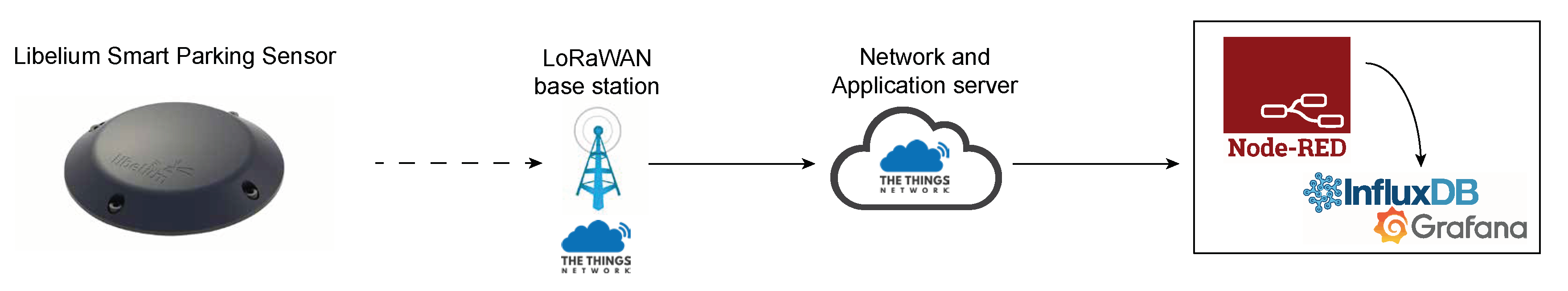
Figure 1 depicts the architecture of implemented LoRaWAN parking mechanism. The core of a Smart Parking sensor device is a commercial LoRaWAN-based Smart Parking sensor device from Libelium that comprises radar and magnetometer sensor for parking lot occupancy detection. These nodes are equipped with waterproof enclosure and they are fully powered with built-in lithium-thionyl chloride (Li-SOCl2) batteries with an overall capacity of 10.4 Ah that allows autonomous operation for a couple of years (Libelium: https://www.libelium.com/iot-products/smart-parking/ (accessed on 20 November 2020)). Five Libelium parking sensor devices were placed at the surface of faculty parking lot. In the implementation of Libelium LoRaWAN parking sensor, the device periodically wakes up (every 60 s) and activates internal sensor devices (such as radar, magnetometer) for checking the change in parking status. If parking lot status changes (from free goes to occupied or from occupied to free), the sensor device transmits the message over a radio while using LoRaWAN protocol to the gateway. In addition, Libelium parking devices employ keep-alive message transmissions, where the parking status is periodically sent if parking lot status does not change, for example, during nighttime hours.

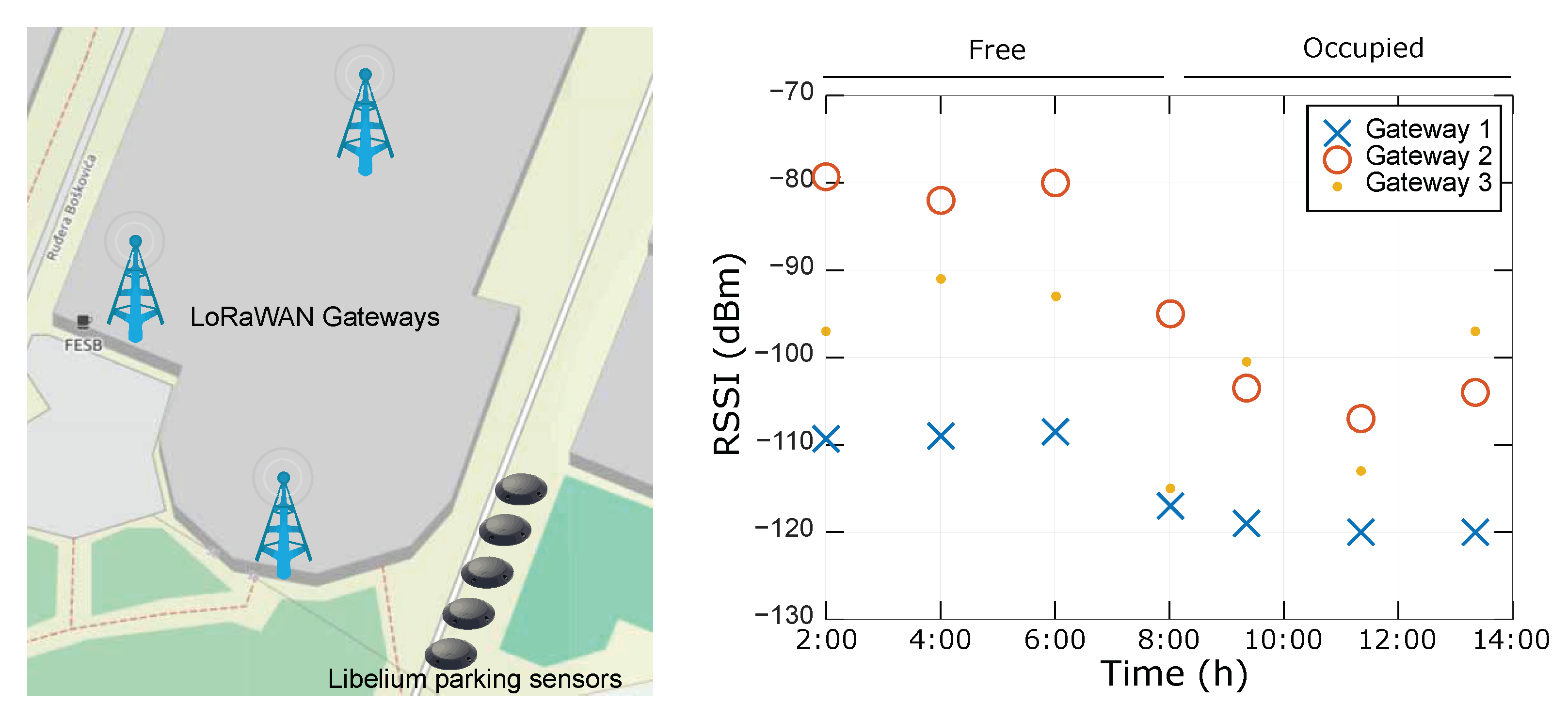
As a LoRaWAN provider, The Things Network (TTN) was selected for its simplicity and good documentation. Furthermore, TTN forwards all of the messages from Libelium Smart Parking sensor to our personal server comprising Node-RED, InfluxDB, and Grafana services for visualization and further processing, as shown in Figure 1. Three TTN gateways were placed within a close vicinity of parking sensor devices, as shown in Figure 2 (left). Once the message arrives to the gateway (the base station), it is forwarded to the TTN Network and Application server, where the message payload is decoded and prepared for further processing and forwarding while using MQTT protocol or HTTP integration. In a given implementation, Node-RED was used for message aggregation from TTN. Afterwards, Node-RED parses and prepares the message for storage in the InfluxDB database. One entry into the database stores information regarding parking lot occupancy, timestamp entry (InfluxDB is a time series database), signal strenght measurements on every gateway device (RSSI and SNR), and sensor ID. Figure 2 (right) shows a snapshot of parking lot occupancy along with RSSI measurement captured on three LoRaWAN gateways. As can be seen, when vehicle occupies a parking lot, a drop in RSSI values is detected at all gateways, which could serve as indicator of occupancy.

Consumption of Libelium Smart Parking Sensor Device

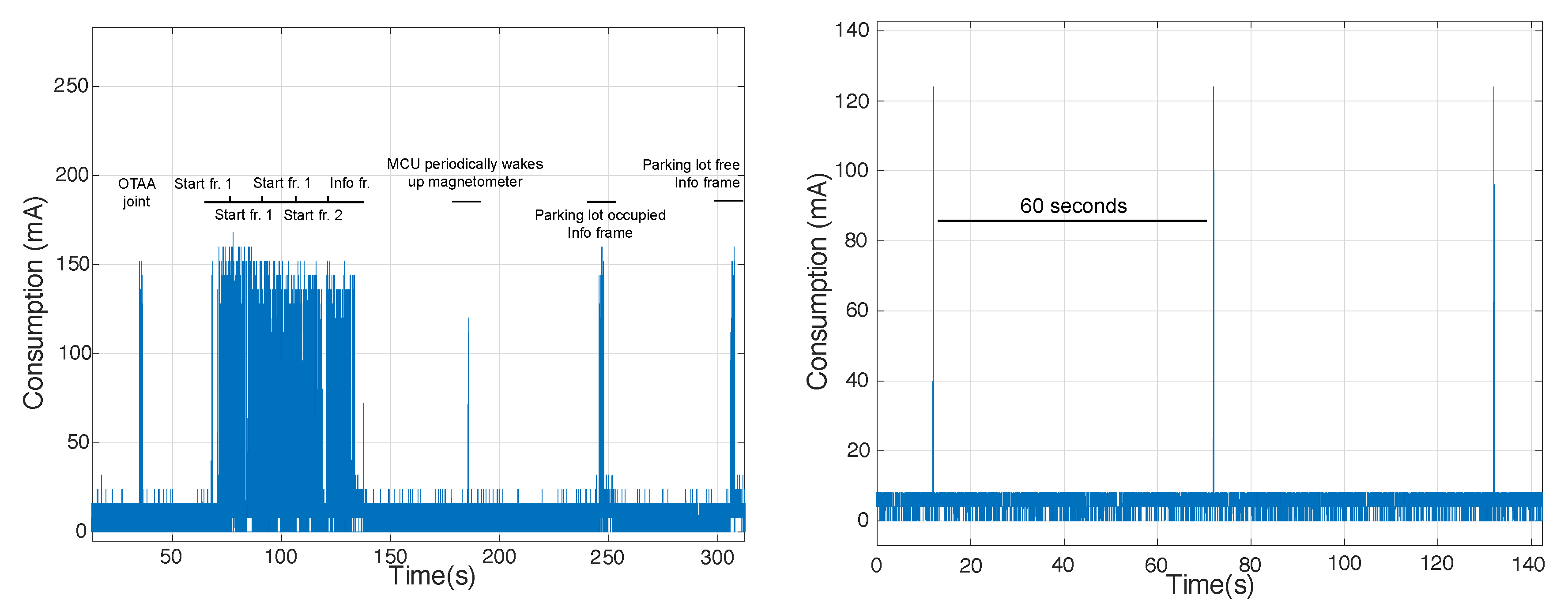
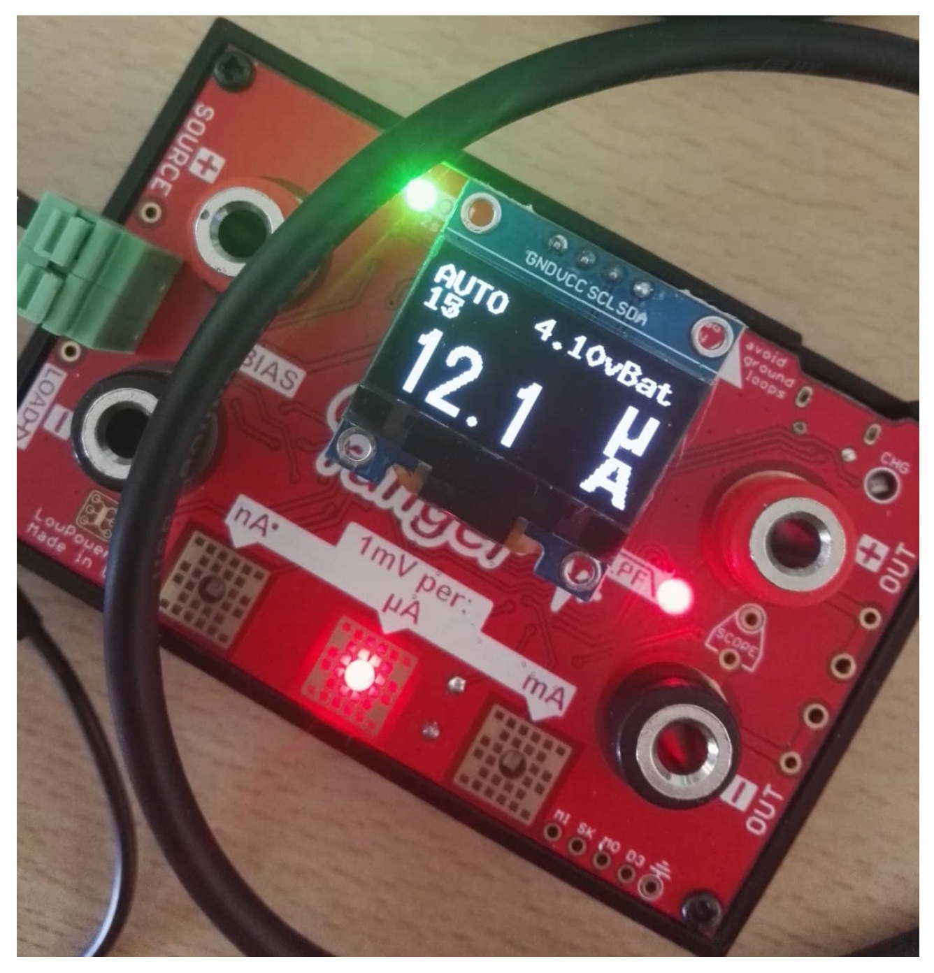
Figure 3 shows the consumption of Libelium smart parking sensor device that utilizes LoRaWAN radio technology for occupancy transmission detection. To capture detailed measurements of current consumption, node was connected to the ooscilloscope via Current Ranger. As can be seen, device first utilizes LoRaWAN OTAA authentication protocol for establishing Network and Application session keys, which is followed by sending two Start frames and Info frame, as specified by the Libelium documentation. During active period, in which node sends occupancy status update, MCU with sensors and radio pheripheral (radar and magnetometer) are powered on, where the overall average consumption will slightly be above 100 mA. In contrast, during inactive period, where MCU with radio pheripheral and sensors is in inactive mode, overall consumption falls to 12 μA (Figure 4). The duty cycle (sleep period) of node is 60 s. After waking up, MCU powers the sensors and checks whether parking status occupancy changed from previous measurement. If parking lot occupancy has changed, MCU wakes up radio for sending status update. Otherwise, a node will enter into sleep mode.

Libelium parking sensor devices are equipped with lithium-thionyl chloride (Li-SOCl2) batteries that have an overall capacity of 10.4 Ah. Assuming consumption in sleep period is 0.012 mA, where device consumption in active period, on average, is 100 mA, along with one LoRaWAN message sent every 60 min and 6 s of wake-up duration, the device lifetime will be 2061.8 days, or 5.65 years. In this calculation, it is assumed that the capacity is automatically derated by 15% from 10.4 Ah in order to account for some self discharge.

4. Beacon-Based LoRaWAN Parking Sensor Device

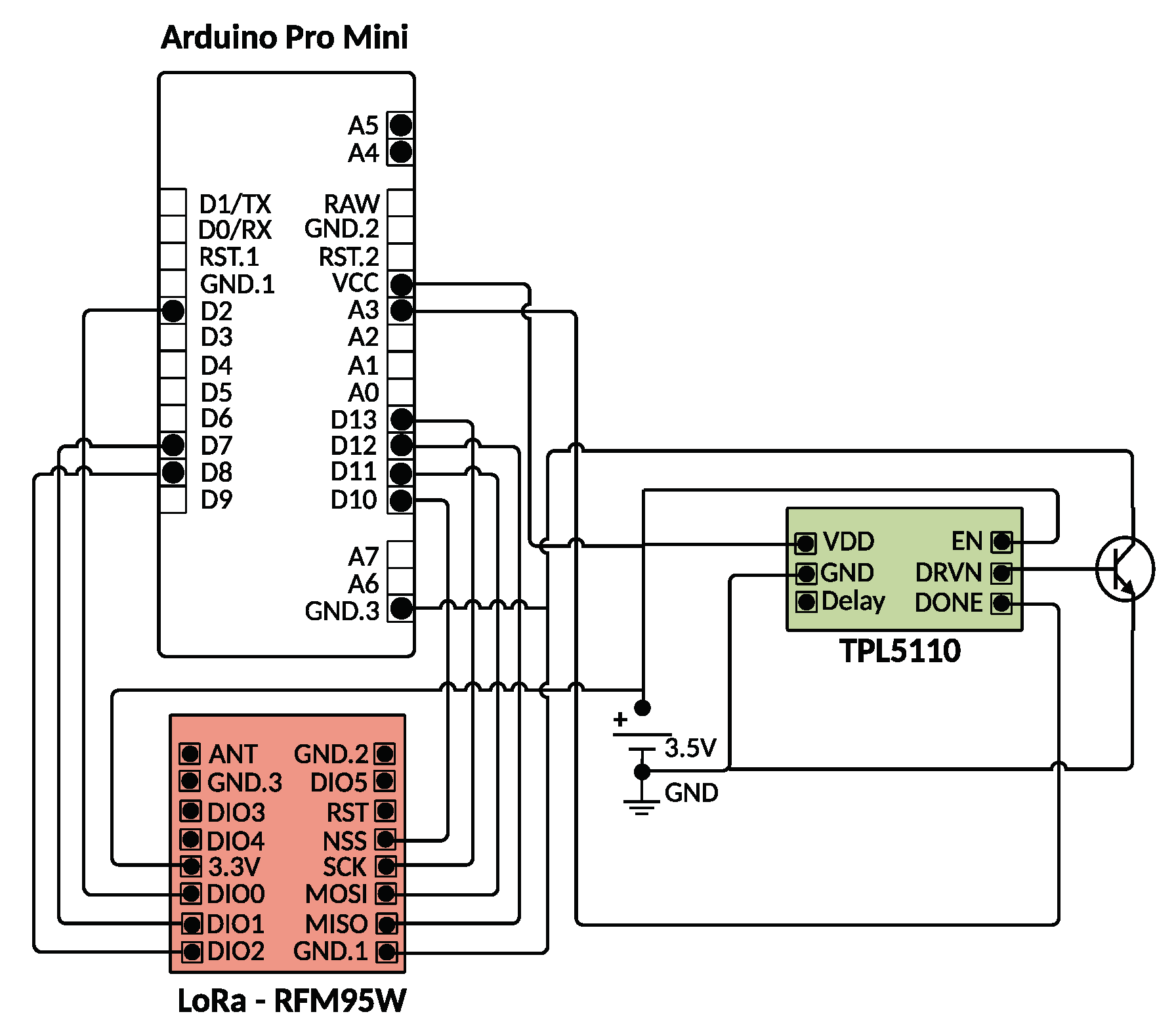
In a concept of a cost effective smart parking occupancy detection device, Machine Learning techniques are employed for estimating occupancy from a beacon device. Such a novel solution will not require any sensor or sensor readings from devices, such as magnetometer and radar employed in Libelium smart parking sensor device. This beacon device would be comprised out of a simple MCU with LoRa radio module, as depicted in Figure 5. In order to minimize energy consumption during inactive period and periodically wake-up MCU from deep sleep, a TPL5110 Nano Timer could be employed. During deep sleep, TPL5110 would cut off power from both the MCU and LoRa module, thus minimizing the overall consumption.

It is necessary to select MCU that supports the library for LoRaWAN message communication. Besides ATmega328P, which is standard MCU for Arduino Uno and Arduino Mini Pro, MCUs that employ libraries for LoRaWAN-based connection are also ATtiny 84, ATtiny 85 and STM32.

Table 2. Comparison of microcontroller (MCU) consumption that support LoRaWAN communication.

MCU	ATmega328P	ATtiny 84	ATtiny 85	STM32F103C8T6 (STM32)
Consumption (3.3. V and 8MHz)	3.9 mA	3 mA	3 mA	8 mA

gives consumption comparison of MCUs during active period. Clearly, for the purposes of creating a simple beacon device, besides ATmega328P, which is found on Arduino Pri Mini, ATtiny 84 or ATtiny 85 could also be used, since their consumption is around 3mA in active state. During inactive state, the TPL5110 Nano Timer is selected, since its consumption is below 1 μA.

Table 3. Consumption of every element of the beacon prototype along with lifetime duration estimation.

LoRa RF96 IC	116.1 mA
Aduino mini pro (ATmega328p)	4 mA
LDO	0.00377 mA
Timer TPL5110	0.000310 mA
Active period duration	5.5 s
Average overall consumption in active period	25 mA
Average consumption in inactive period	4 μA
Lifetime duration (10.4 Ah battery)	1594 days

depicts the energy consumption of every component that builds the Beacon Device. Because the beacon device does not hold any sensor, the active period basically comprises of waking up MCU and LoRa radio module, and sending LoRaWAN message, which can be reduced to approximately 5.5 s. In an active period, the average consumption is 25 mA, which includes 116 mA of consumption during LoRaWAN communication during a smaller portion of time, and 3 mA of MCU consumption during active period. Note that LoRa communication only occupies small portion of active period. During deep sleep period, device consumption could be around 4 μA, which includes TPL5110 timer and low power voltage regulator. Assuming a duty cycle of 10 min., with a battery capacity of 10.4 Ah and 15% self discharge, the battery lifetime should be approximately 4.33 years.

Table 4. Price of the overall beacon device.

Module	Price (USD)
ATMega328P Pro Mini	1.57
RFM95	4.18
DS3231	1.02
Overall	6.77

shows price of the proposed beacon device, and its components used in its development. As an alternative to TPL5150 timer, DS3231 low-power and low-cost RTC clock could be used in order to periodically wake-up Arduino from deep sleep which can lower the consumption of the complete beacon to below 1 μA. The DS3231 can be found for a price of around 1 USD. Microcontroller that supports LoRaWAN library is ATMega328P, whereas its representative, Pro Mini, can be found in a price range of around 1.5 USD. In order to convey information over the radio, RFM95 LoRa module could be employed, with price of approximately 4.18 USD. Hence, the overall price of the module goes below 7 USD. For comparison, the price of FMCW Radar sensor device that is typically found in Libelium smart parking device is 14 USD, i.e., twice the price of the developed beacon device. Taking the price of magnetometer as well as the MCU and timer into account, the overall price goes well above the price of the proposed beacon device.

5. Experimental Setup and Data Analysis

5.1. Experimental Setup

For the purpose of collecting parking occupancy detection, five Libelium Smart Parking sensor devices were placed at the faculty parking lot next to each other (Figure 2 (left)). These parking sensor devices are placed in the center of the parking lot at the surface. The devices are equipped with a magnetometer and radar sensor devices, in such a way that, when the parking lot status changes (when vehicle approaches or leaves the parking lot), the sensing technology detects change and sends information over a radio channel. As a communication peripheral, Libelium devices employ LoRa radio capabilities in order to convey information regarding changes in parking lot occupancy. Besides sensing event driven packets, Libelium sensors also send keep-alive packets periodically every two hours. Three LoRaWAN gateways were placed in the radio range of Libelium parking sensors in order to collect data from Libelium devices. Two gateways were placed indoor within faculty facilities, while the third gateway was placed outdoor on top of the faculty. Namely, the first gateway was placed on the faculty first floor (4 m from the ground and around 30 m from the sensor), the second gateway was placed at the faculty fifth floor (around 15 m from the ground and 75 m from the sensor), while the third gateway was placed on the ninth floor of the faculty (around 30 m from the ground and 145 m from the sensor), as can be depicted in Figure 2 (left). Installed gateways employ TTN technology that allows for the collection of data from gateways and their storage into a designated database. The data were stored into the InfluxDB database, as shown in Figure 1. The collected data comprised information about parking lot occupancy status, Received Signal Strength Indicator (RSSI) in dBm, Signal to Noise Ratio (SNR) for every gateway, Gateway ID, Sensor ID, as well as the timestamp of the moment at which the data were received by TTN gateway. The data have been collected from five different sensors and three different gateways in period from 13th of December 2019 until 6th of September 2020. During that period, 130,984 raw data were collected from all five sensors. InfluxDB further allowed for the exportation of the collected data into csv. format for further processing. Machine learning techniques were employed on the collected data while using dedicated computing machine for performing such a task. Namely, Intel core [email protected] processor with 8GB of RAM and NVIDIA GTX1050 GPU running 64 bit Windows 10 operating system has been used. NVIDIA CUDA Deep Neural Network library (cuDNN) was employed to utilize the performances of fast computing using GPU. The Keras 2.3.1. Python library was used running on top of a source build of Tensorflow 2.2.0 with CUDA support.me for different batch sizes.

5.2. Data Analysis

Because all of the gateways did not receive the same amount of data and, moreover, not in the same timestamp, it was decided to extract relevant data for each sensor and each of the three different gateways separately for the analysis.

In accordance with the goal of detecting how Occupancy Status is related with Received Signal Strength Indicator and Signal to Noise Ratio, it was proceeded with a plotting of the histograms presented in Figure 6 in order to gain a general illustration of the relationship between the aforementioned variables.

Firstly, it was noticed that parking lots are free considerably more than they are occupied. This is an important property of the parking place indicating its stochastic behavior. The parking is located on University grounds and, therefore, is usually free during night time or over the weekend periods. Secondly, the histograms depict that the RSSI values for free and RSSI values for occupied parking status overlap in Gateway 1 (GW1) and Gateway 2 (GW2). The same reasoning applies for SNR values for all sensors in GW1 and GW2. However, result that were gained for Gateway 3 (GW3) and sensors 2, 3, and 4 differ from above mentioned. The aforementioned sensors gave the least overlapping of RSSI and SNR values for a particular occupancy state. It was also noticed that higher RSSI values indicate a free parking space, while lower indicate the occupied one. The difference between the results gained for different gateways could be a consequence of the distance of GW1 (30 m), GW2 (75 m), and GW3 (145 m) from the parking sensor. GW3 is furthest away and on top of the University building and outdoor. This would imply that the closer the gateway, the channel influences RSSI and SNR stronger than the change of the parking status.

Because of the overlapping of RSSI and SNR values in different occupancy states, it was important to explore the change of RSSI and SNR values when the parking status does not change and when it changes from one state to another. Further analyses showed that, when parking status does not change, the values of RSSI and SNR change very little or not at all. However, when the parking status does change, there is a significant change in the RSSI and SNR values. Figure 7 presents histograms of changes of values for RSSI when parking space remains free and when parking space becomes occupied prior to being free for sensor 2 from GW3.

In light of the above reasoning, the conclusions were twofold: (1) RSSI, SNR, and occupancy status are considerably correlated and (2) the adequate ML algorithm must be able to comprise the complexity of the data correlations in order to provide an appropriate estimation of occupancy status.

6. Machine Learning as an Approach to Parking Occupancy Detection

In the IoT paradigm of numerous smart connected devices, Machine Learning has emerged as an essential field of research and application aiming at providing computer programs the ability to automatically improve through experience [47]. The most distinguished attribute of a learning machine is that the trainer of learning machine is ignorant of the processes within it [48]. Machine learning generally includes data processing, training, and testing phases with the aim of making the system able to carry out decisions based on the input received from the training phase [13]. In order to archive the learning process, systems use various algorithms and statistical models to analyze the data and gain information about the correlation between the data features [12]. The algorithms that are used in these processes can be divided into four distinctive groups, as Supervised, Unsupervised, Semi-supervised, and Reinforcement learning algorithms:

• Supervised learning algorithms demand external monitoring by a supervisor with the goal of learning how to map input values to the output values where the accurate values are given by a supervisor [49].
• Unsupervised learning algorithms make computers learn how to perform a specific task only with the provided unlabeled data. These types of algorithms need to find existing relationships, irregularities, similarities, and regularities in provided input data [50].
• Semi-supervised learning is a hybrid approach of the previous two categories that uses both labeled data and unlabeled data. These algorithms generally act like the unsupervised learning algorithms with the improvements that are brought from a portion of labeled data [51].
• Reinforcement learning algorithms operate with a restricted insight of the environment and with limited feedback on the quality of the decisions. In order to operate effectively and provide the most positive outcome, these algorithms have the ability to selectively ignore irrelevant details [52].

ML has been ideally suited for various types of problems, such as as classification, clustering, predictions, pattern recognition, etc. The most appropriate ML algorithm is chosen based on the swiftness of the technique and its computational intensity, depending on the application type [12].

Nowadays, Deep Learning (DL) has become one of the leading Machine Learning techniques efficient in solving complex problems that have otherwise been impossible to solve while using more traditional ML approaches [13]. Deep Learning has been recognized as one of the ten breakthrough technologies of 2013 and fastest-growing trend in big data analysis [53]. Deep Learning applications have achieved remarkable accuracy and popularity in various fields, especially in image and audio related domains [13]. Deep Learning (DL) techniques effectively give insights from the data, comprehend the patterns from the data, and classify or predict the data [54]. Neural Networks that involve more than two hidden layers have been considered to be a characterization of DL and the word ’deep’ signifies the large number of hidden layers that compose the Neural Network [53]. Implementations of Deep Learning technology today is achieving a large success in a variety of engineering and technical problems, including object detection, traffic engineering, traffic classification, and prediction [23,55,56,57].

6.1. Hidden Markov Model

Hidden Markov Models (HMMs) have been known for decades and, today, are making a large impact with regard to their applications, especially in form of Machine Learning models and applications in reinforcement learning. They are widely being used for pattern recognition [58], i.e., namely speech recognition [21] as well as in biological sequence analysis [59], gene sequence modeling, activity recognition [60], and analyses of ECG signal [61,62]. Markov Chains and process were first introduced by Markov in 1906 as a time-varying random phenomenon for which the Markov properties are attained. Its practical importance is the use of the hypothesis that the Markov property holds for a certain random process in order to build a stochastic model for that process [22].

In the broadest sense, a Hidden Markov Model (HMM) is a Markov process that can be divided into two parts: an observable component and an unobservable or hidden component. The observation is a probabilistic function of the state, i.e., the resulting model is a doubly embedded stochastic process, which is not necessarily observable, but it can be observed through another set of stochastic processes that produce the sequence of observations. A machine learning algorithm can apply Markov models to decision making processes regarding the prediction of an outcome.

In 1986, Rabiner and Juang [63] gave the structure of the first order Hidden Markov Model, denoted as $\lambda \left(A,B,\pi \right)$, where $A=\left\{a_{ij}\right\}$ is the matrix of transition probabilities, $B=\left\{b_j\left(k\right)\right\}$ is the matrix of observation probability distribution in each state, and $\pi$ is the initial state distribution. Rabiner (1989) presented [64] three different types of problems in HMM: The Evaluation Problem, Decoding problem and Learning. The first problem is commonly solved by using the Forward or Backward algorithm, where as the last problem is, the most difficult of the three problems, usually solved while using Baum–Welch method. With regards to the second problem, the central issue is to find the optimal sequence of states to a given observation sequence and model used. The most common method to this is by using the Viterbi algorithm, which was introduced by Andrew Viterbi in 1967 as a decoding algorithm for convolution codes over noisy digital communication links. It is the answer to the decoding problem resulting in the Viterbi path, since the algorithm can be interpreted as a search in a graph whose nodes are formed by the states of the HMM in each of the time instant [22]. Let $\lambda \left(A,B,\pi \right)$ be a HMM and $O=(o_1,o_2,\dots ,o_T)$ given observations. The Viterbi algorithm finds the single best state sequence $q=(q_1,q_2,\dots ,q_{{}_T})$ for the given model and observations. The probability of observing $o_1,o_2,\dots ,o_t$ using the best path that ends in state i at the time i given the model $\lambda$ is:

$${\delta }_t\left(i\right)=\underset{q_1{,q}_2{,\dots ,q}_{t-1}}{max}\mathbb{P}(q_1,q_2,\dots ,q_{t-i},q_t=i,o_2,o_2,\dots ,o_t\mid \lambda )$$

(1)

${\delta }_{t+1}\left(i\right)$ can be found using induction as:

$${\delta }_{t+1}\left(i\right)=b_j\left(o_{t+1}\right)\underset{1\le i\le N}{max}\left[{\delta }_t\left(i\right)a_{ij}\right]$$

(2)

In order to return the state sequence, the argument that maximizes Equation (2) for every t and every j is stored in a array ${\psi }_t\left(j\right)$ [63]. It is important to point out that the Viterbi algorithm can be directly implemented as a computer algorithm. Moreover, the algorithm succeeds in splitting up a global optimization problem, so that the optimum can be computed recursively: in each step, we maximize over one variable only, rather than maximizing over all n variables simultaneously.

Hidden Markov Models have been used now for decades in signal-processing applications, such as speech recognition, but the interest in models has been broaden to fields of all kind of recognition, bioinformatics, finance etc. [65].

With regards to the first order Markov model, if the past and the present information of the process is known, the statistical behavior of the future evolution of the process is determined by the present state. Thus, the past and future are conditionally independent (the system has no memory) [66]. Therefore, it is reasonable to ask whether there can be a model that can gather and somewhat keep information from the past. The answer lies within a higher-order Markov models, where the hidden process is a higher order Markov chain and it is dependent on previous states. This gives memory to the model and such a modeling is more appropriate for processes in which memory is evident and important, for example, a stock market time series.

Model and Results

The collected and visualised data, as presented in Data analyses section, revealed the general proprieties of our data, their correlation, and enabled us in designing the appropriate model for the Machine Learning approach in reaching the desired goal. The aim is to determine the occupancy of a parking space based solely on Received Signal Strength Indicator and Signal to Noise Ratio values. Hidden Markov Model of second order, which is presented in the following, was designed and used in order to classify the occupancy status of a parking space, while using RSSI and SNR values.

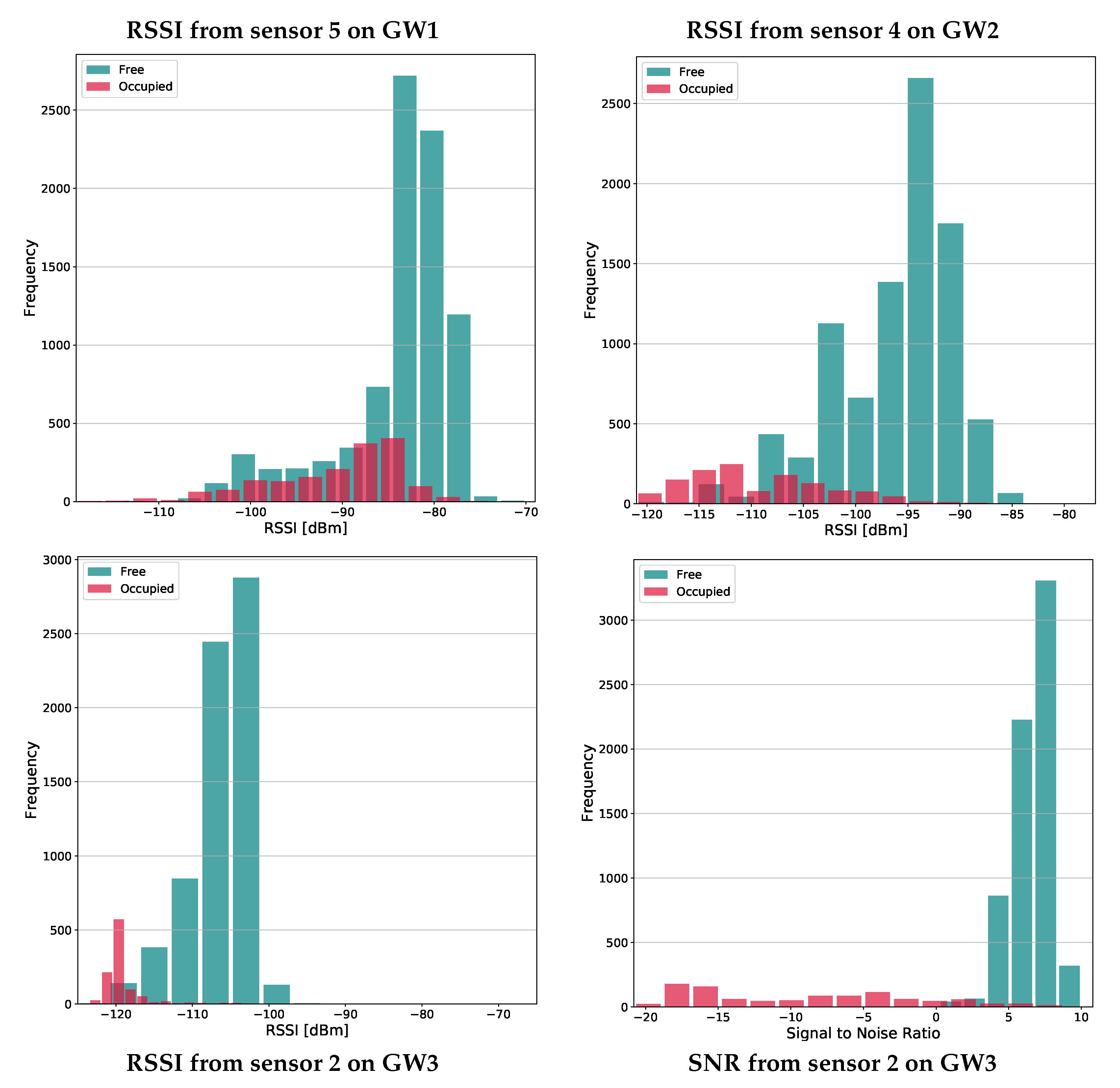
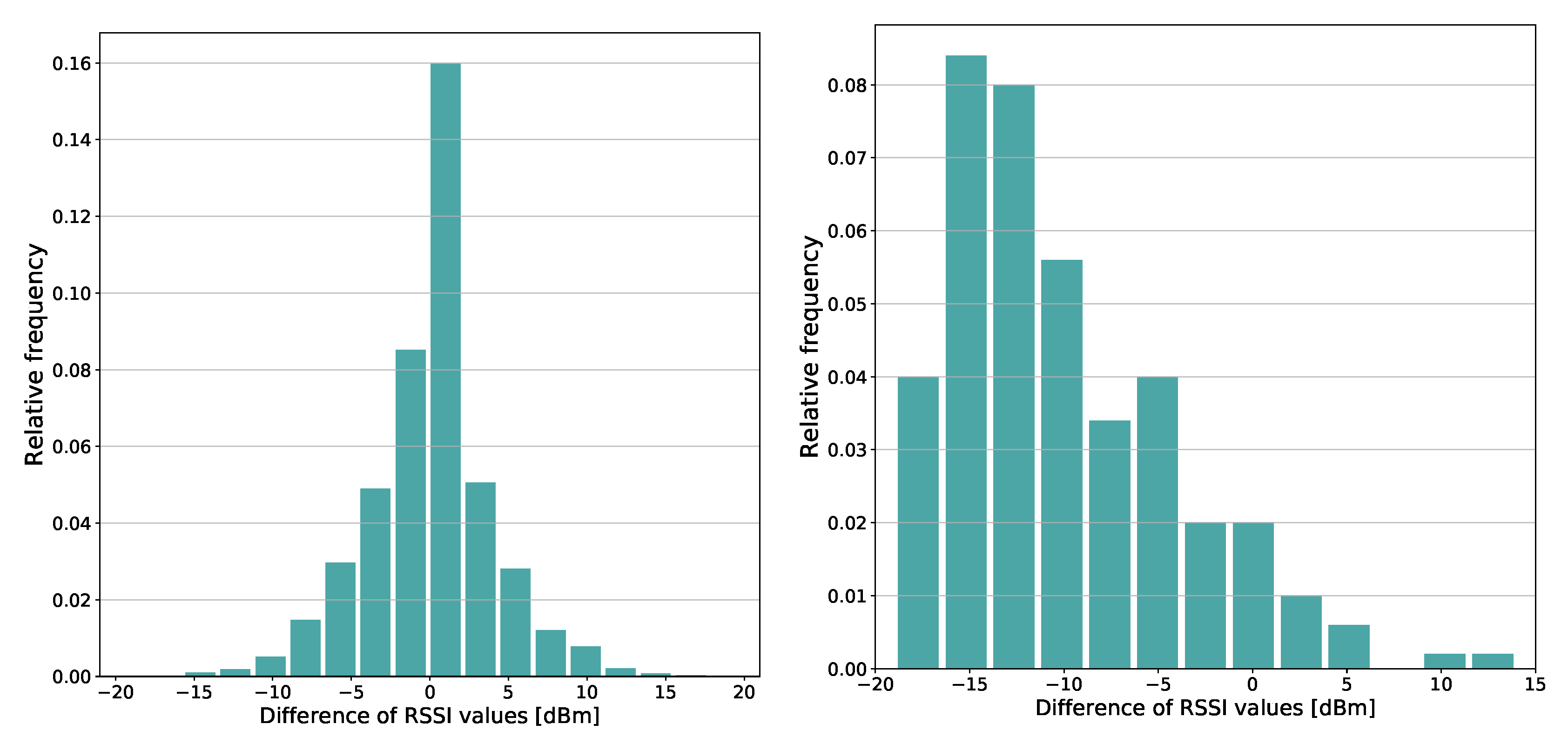
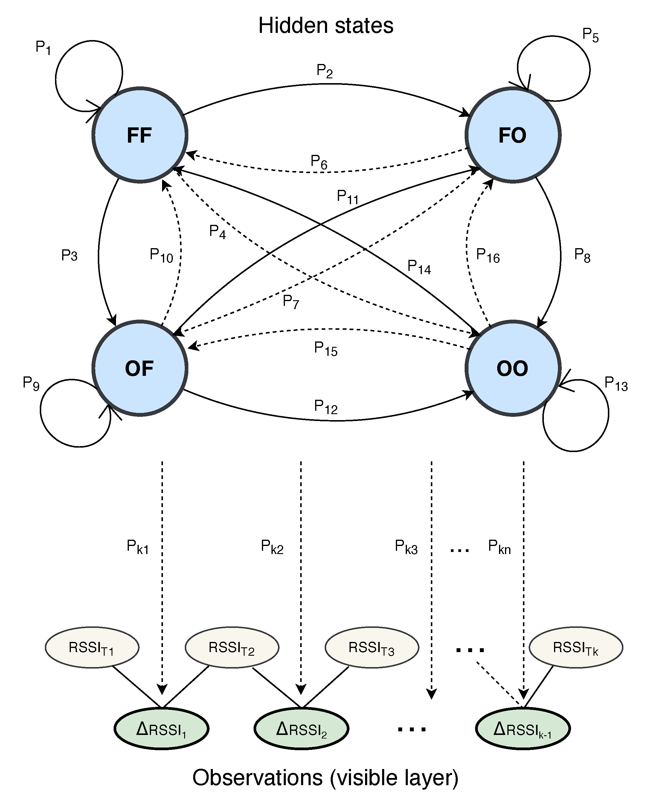
From previously presented and discussed histograms of RSSI and SNR values with regards to occupancy status, it was concluded that, when parking status does not change, the values of RSSI and SNR change very little or, in most cases, not at all. In contrast, when the parking status does change, there is a significant change in RSSI and SNR values. Therefore, the variables “bring memory” with them that is dependent of the previous state of occupancy. The process it self is of a time series that can be designed and modeled using a second-order HMM. In this model, the Hidden States are the aim of prediction, which is Occupancy status. In order to “bring memory” into our model, the Observable (Visible) States are defined to be the changes of RSSI (the same reasoning and model applies for SNR) values that are calculated as the difference between these values from two previous states. The notation and model illustration are as follows:

• F—free, O—occupied.
• RSSI_s—value of Received Signal Strength in occupancy state s in a timestamp.
• ΔRSSI = RSSI_s − RSSI_s+1. Difference between two values of RSSI in two consecutive occupancy states.
• FF—state that is free which previous state was free.
• FO—state that is occupied after previously being free.
• OF—state that is free after being occupied
• OO—state that is occupied which previous state was occupied.

States FF, FO, OF, and OO bring with them “memory of occupancy”, since they remember what was the occupancy status form the “past”. These states represent Hidden Layer of states. The Hidden Markov Model model is denoted as $\lambda \left(A,B,\pi \right)$, where:

• A is the transition matrix. It stores probabilities of transition from one state to another. The matrix holds some zero values, due to the fact that some transitions are impossible. For instance, you cannot transit from state $FF$ into the state $OO$,
• π is the initial state distribution (stationary distribution) and it is calculated by solving the matrix equation

  $$\pi =\pi ·A.$$
• B is the matrix containing the observation probability distribution in each state. In this model, the observations are the changes of $RSSI$ values in two consecutive occupancy states—$\Delta RSSI$.

Figure 8 visualizes the architecture of our second order HMM.

As stated, because it was decided to extract the relevant data for each sensor and each of the three different gateways separately, the implementation took all of these possibilities into account. The used decoding algorithm for finding the optimal sequence of states to a given observation sequence and model is previously defined Viterbi algorithm. All of the data were effectively used as an observation for a chosen step and given as input to the Viterbi algorithm. The chosen step determines the length of observation sequence. For example, if the chosen step is 4, then the whole data set from selected sensor and gateway is divided into subsets of sequences containing four consecutive values of a chosen variable (RSSI or SNR). Every one of this sequences is then given as an observation input to the Viterbi algorithm.

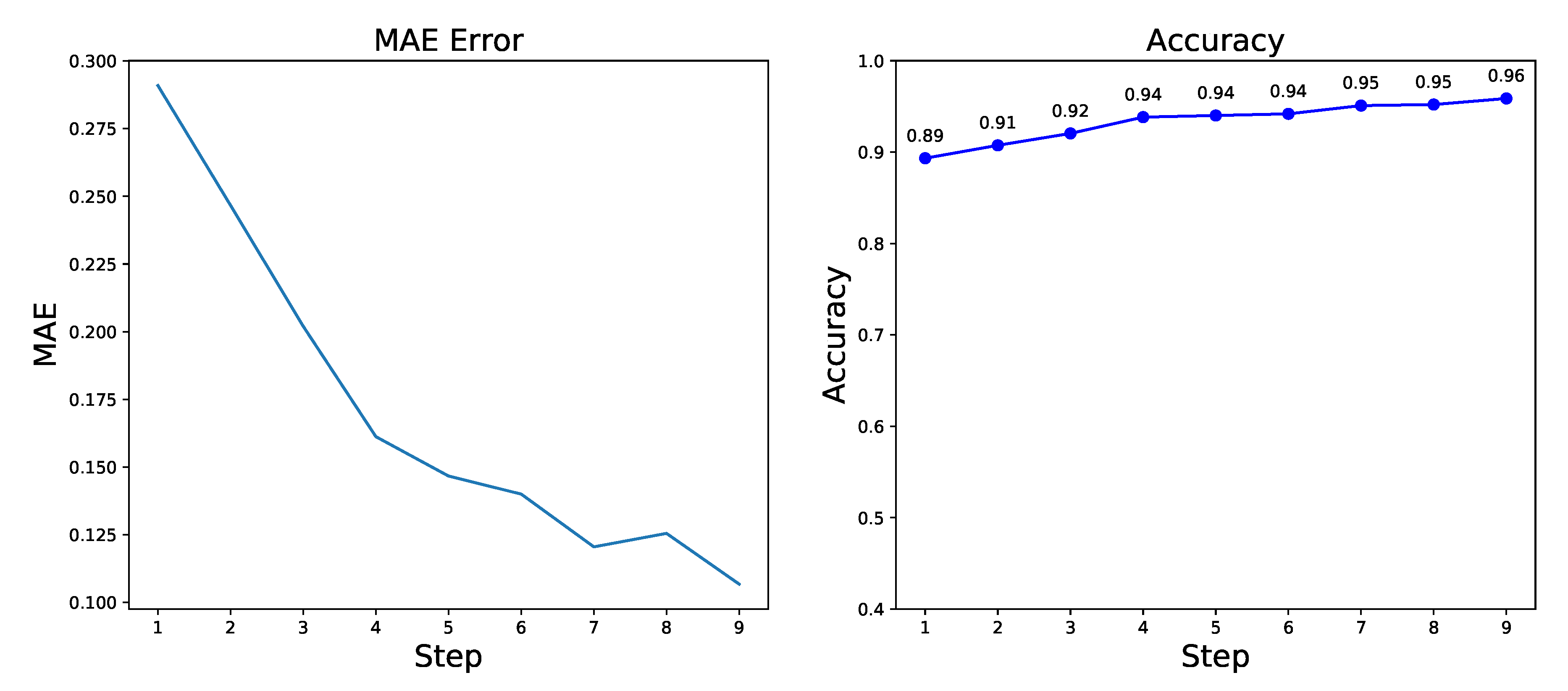
The classified and the true values are stored separately and the accuracy is calculated while using accuracy score function. This function computes subset accuracy, which is the fraction of samples classified correctly. The set of labels classified for a sample must exactly match the corresponding set of labels of true values. Moreover, the model’s evaluation is done while using Mean Absolute Error (MAE). The model was tested for all variables from all sensors and gateways, and the best results are given in

Table 5. Table of best results using the Hidden Markov Model (HMM) model obtained for each gateway.

Gateway	Variable (Sensor Number)	Accuracy (Best Results)	MAE
GW1	RSSI (4)	87%	0.30
GW1	SNR (4)	87%	0.35
GW2	RSSI (3)	89%	0.27
GW2	SNR (3)	92%	0.20
GW3	RSSI (2)	93%	0.17
GW3	SNR (2)	96%	0.11

.

The least promising results were gained form the closest gateway GW1, as can be seen from the table. On GW1, the second HMM model only reached 87% accuracy with a MAE of 0.30. This is due to the previously explained overlapping in the RSSI (or SNR) values with regards to different occupancy status. With regards to GW2, the best results are slightly better with regards to Accuracy and MAE than GW1. This also is consistent with the reasoning of overlapping values for different occupancy status.

Finally, the best results were obtained for the furthest GW3, giving 96% accuracy for observation values of SNR from sensor 2 and senor 4 and MAE of 0.17 and 0.11, respectively. Figure 9 illustrates the best result that is obtained while using the HMM model from sensors 2 from Gateway 3.

Despite the results that were obtained while using the second order HMM, this approach has limitations; the states must be drawn from a modestly sized discrete state space and each hidden state can depend only on the immediate previous state [26]. In order to model N bits of information about the past history, HMM requires $2^N$ hidden states [67], which makes it computationally impractical for large data sets. HMM are generative classifiers which means that they explicitly model the actual distribution of each class, in contrast to discriminative models, such as Neural Networks, which model the decision boundary between the classes [68]. Discriminative models can provide robust solutions for non-linear discrimination in high-dimensional spaces [69] and they have been shown to be quite effective for applications in classification [70]. Therefore it reasonable to examine Neural Networks as another approach that can encompass complex, high-dimensional, and noisy real-world data.

7. Neural Network Models

Neural Networks, or Artificial Neural Networks (ANN), have gained significant attention in the last two decades as a Machine Learning technique in a variety of areas for prediction and classification task [12]. Inspiration for their architecture was taken from the brain nervous system in a form of a mathematical model that is designed to mimic the structure and functionalities of the real biological Neural Networks [71]. They have been applied in many divers areas of scientific research, such as pattern recognition [72], image classification [73], language processing [74], computer vision [75], as well as time series forecasting [76].

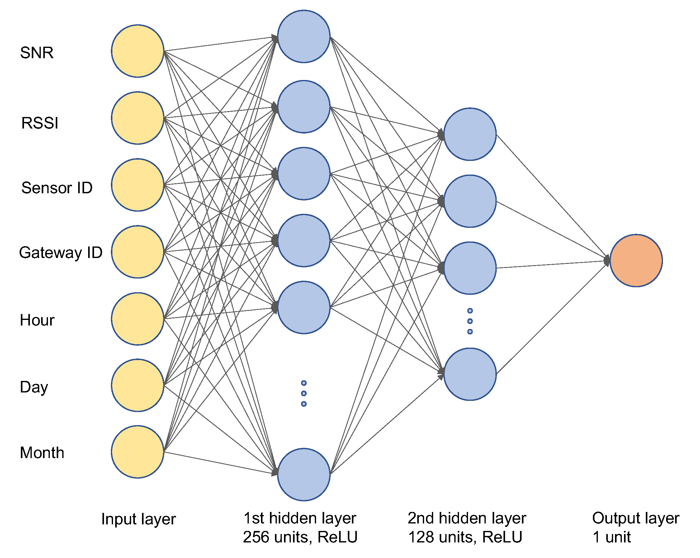
Generally, the Neural Network consists out of three basic layers as shown in Figure 10, namely the input layer, the hidden layers, and the output layer. The Neural Network can have more than one hidden layer, which represents the depth of the Neural Network. The imitation of the brain learning processes is done by searching the hidden links between a series of input data while using hidden layers of neurons, where the output of a neuron of a layer becomes the input of a neuron of the next layer. An artificial neuron $y_i$ can be defined as a function

$$y_i=f_i\left(x\right)=\phi (〈w_i,x〉+b_i),$$

(3)

which acts on a linear combination of the input vector $x=(x_1,...,x_n)$ and a neuron bias $b_i$ [77]. The input vector is weighted with the connection weight vector $w_i=(w_{1,i},...,w_{n,i})$ and the $\phi$ is called activation function. The performance of the training process and estimation (or prediction) accuracy of the NN is highly influenced by the weight initialization and activation function [78]. The activation function will control the amplitude of the output of the neuron, keeping it in a usually acceptable range of $[0,1]$ or $[-1,1]$ [79]. The activation functions are divided into linear and non-linear activation function and non-linear ones are most commonly used. Some of most frequently applied non-linear activation functions are Sigmoid, Rectified Linear Unit (ReLU), and Tanh function. Sigmoind function can be defined as $S\left(x\right):\mathbb{R}\to [0,1]$

$$S\left(x\right)=\frac{1}{1+e^{-x}}.$$

The Sigmoid function is continuously differentiable, but it suffers from gradient vanishing [78], which can significantly slow down the learning process. This problem has been resolved while using the ReLU activation function.

ReLU function can be defined as $\varphi :\mathbb{R}\to {\mathbb{R}}^{+}$

$$\varphi \left(x\right)=\left\{\begin{array}{c}\lambda x,x>0\\ \beta x,x\le 0\end{array}\right.,$$

where commonly $\lambda =1$ and $\beta =0$. The derivative of the function will be quite simple, 1 for positive values and 0 otherwise, as can be seen from the function’s definition. Therefore, the average derivative is rarely close to 0, which allows gradient descent to keep progressing. Hence, ReLU has been mainly used as an activation function for the neurons that are placed in hidden layers [78], while Sigmoid has been used as a activation function for the neurons that are placed in the output layer. This paper implements a Neural Network comprised out of two hidden layers (Figure 10). The input layer takes data, such as the sensor ID, RSSI, and SNR, of the LoRa packet sent from the sensor to the Gateway, and ID of that gateway, along with the timestamp of the event when the packet was sent. The exit layer predicts parking space occupancy (free or occupied).

As seen, the layers comprise artificial neurons, where every neuron has multiple weights and some form of transfer or activation function. The Neural Network is a supervised learning algorithm, in which the weight of the neurons is calculated during the training process. Because of the training procedure, the input data to the network should cause the output as close to the ground truth. In order to accomplish this, during the training procedure, which is an iterative procedure, a loss (cost) function is used to determine the quality of the network with specific weights. For a binary classification problem, such as parking lot occupancy, Binary Cross-Entropy Loss, as one of the commonly used loss functions, and it has been utilized in this research.

In order to minimize loss function during the training phase in which the weight of neurons is determined, a good deal of optimization algorithms have been implemented, many of which are first-order iterative optimization algorithms. The algorithms used in this paper were Stochastic Gradient Descent (SGD), Adaptive Moment Optimization (Adam), and Root Mean Square Propagation (RMSProp).

7.1. Evaluation Metrics

The proposed Neural Network model has been evaluated while using different metrics to evaluate different characteristics of the classifier. Namely, the metrics used were Accuracy, F1 score, Area under the Receiver Operating Characteristic Curve Accuracy (ROC AUC) and Average Precision (AP).

• Accuracy—it is defined as the overall accuracy or proportion of correct predictions of the model and it is given with the formula:

  $$Accuracy=\frac{TP+TN}{TP+FP+TN+F{N}^{\prime }}$$

  (4)

  where TP and TN denote the number of positive and negative instances that are correctly classified. FP and FN denote the number of misclassified negative and positive instances, respectively.
• F1 score—F1 score is the harmonic mean of the Precision and Recall. Precision is defined as the number of correct predictions out of all the predictions based on the positive class, whereas Recall is the number of instances of the positive class that were correctly predicted [13]. F1 score is calculated while using formula:

  $$F1score=2·\frac{Precision·Recall}{Precision+Recall}.$$

  (5)

  The F1 score takes values from the $[0,1]$ interval, reaching minimum for TP = 0, that is, when all the positive samples are misclassified, and the maximum for FN = FP = 0, which is for perfect classification [80].
• ROC AUC—the Receiver Operator Characteristic (ROC) curve is an evaluation metric for binary classification problems and it is a probability curve that is created by plotting the True Positive Rate (TPR) versus the False Positive Rate (FPR) [13]. The Area Under the Curve (AUC) represents a separability measure of classifiers, i.e., the ability of the classifier to distinguish between classes [81]. The ideal classifier will have the unit area under the curve and a worst case classifier will have FPR = 100% and TPR = 0 [13].
• Average Precision—it is the measure that considers both Recall and Precision and can be expressed as a function $p\left(r\right)$ of the recall and it is given with [82]:

  $$AveragePrecision=\underset{0}{\stackrel{1}{\int }}p\left(r\right)dr.$$

  (6)

7.2. Results and Discussion

Data used for building the NN model were previously described in Data Analysis section. The pre-processing of data comprised of data normalization due the different value scales of variables in the collected data. The inputs to the model were values of RSSI and SNR for a specific sensor and gateway, whereas the target values were numeric values of parking lot occupancy (0—free, 1—occupied). Therefore, for each of the sensors, data from all three gateways were given as input. There is a slight imbalance regarding the number of instances of each class, depending on the sensor and gateway, as was observed in Data Analyses section. This does not represent a problem for (GW3), since it gives the smallest overlapping of RSSI and SNR values for a particular occupancy state, and good results can be obtained, regardless of class disproportion, if both groups are well represented and their distributions do not entirely overlap [83]. Therefore, the data were first split into training and test set while using stratification in order to preserve the distribution of classes in training and test set, with the test set size being 10%. Moreover, the training set was further split into train and validation set also using stratification, with the validation set size being 10%. Stratification will equalize the ratios of the number of training and validation samples for each class and it is able to achieve lower biases and small variances in estimated accuracies [84], providing consistent predictive performance scores. This way, potential biases that could be caused by the some imbalance in the data set are minimized.

Different optimizers, namely, Adaptive Moment Optimization (Adam), Root Mean Square Propagation (RMSprop), and Stochastic Gradient Descent (SGD), were tested, as well as other hyper-parameters that are presented in

Table 6. Selection of the hyper parameters for evaluation.

Hyper Parameter	Values
Number of neurons	Layer1—256, Layer2—128
Learning rate	0.001, 0.01
Number of epochs	50, 100, 150
Batch size	64

.

The first experimental results of the Neural Network model exposed that Adam, as an optimizer, has achieved the best performance results. This is reported for all sensors in

Table 7. Results of first Neural Network model for Adaptive Moment Optimization (Adam) optimizer.

Sensor ID	Learn. Rate	Epochs	TRAINING				VALIDATION				TEST
			Acc.	F-Score	AUC	AP	Acc.	F-Score	AUC	AP	Acc.	F-Score	AUC	AP
1	0.001	50	0.885	0.471	0.896	0.638	0.883	0.503	0.925	0.750	0.869	0.448	0.892	0.647
1	0.001	100	0.885	0.546	0.904	0.662	0.889	0.551	0.891	0.634	0.897	0.570	0.908	0.679
1	0.01	50	0.879	0.395	0.898	0.635	0.869	0.412	0.899	0.646	0.874	0.394	0.892	0.626
1	0.01	100	0.883	0.512	0.893	0.633	0.880	0.522	0.908	0.674	0.879	0.538	0.907	0.651
2	0.001	50	0.911	0.576	0.934	0.749	0.921	0.608	0.931	0.745	0.914	0.573	0.938	0.749
2	0.001	100	0.915	0.592	0.935	0.754	0.911	0.590	0.936	0.765	0.915	0.587	0.942	0.766
2	0.01	50	0.912	0.546	0.935	0.753	0.913	0.527	0.934	0.742	0.905	0.512	0.929	0.742
2	0.01	100	0.911	0.547	0.931	0.745	0.917	0.585	0.937	0.771	0.914	0.566	0.932	0.734
3	0.001	50	0.912	0.601	0.933	0.744	0.908	0.621	0.940	0.781	0.911	0.568	0.928	0.720
3	0.001	100	0.913	0.560	0.916	0.714	0.913	0.560	0.901	0.718	0.906	0.519	0.906	0.711
3	0.01	50	0.911	0.540	0.911	0.708	0.906	0.487	0.902	0.675	0.919	0.575	0.911	0.716
3	0.01	100	0.911	0.525	0.912	0.702	0.912	0.557	0.918	0.743	0.919	0.571	0.902	0.717
4	0.001	50	0.937	0.749	0.952	0.833	0.940	0.756	0.956	0.847	0.937	0.750	0.945	0.835
4	0.001	100	0.935	0.729	0.953	0.838	0.943	0.758	0.959	0.858	0.936	0.701	0.957	0.838
4	0.01	50	0.936	0.745	0.954	0.840	0.937	0.733	0.943	0.802	0.935	0.738	0.946	0.819
4	0.01	100	0.935	0.729	0.956	0.836	0.933	0.708	0.956	0.823	0.941	0.762	0.959	0.856
5	0.001	50	0.852	0.306	0.807	0.555	0.862	0.343	0.829	0.585	0.845	0.311	0.816	0.566
5	0.001	50	0.852	0.312	0.814	0.566	0.854	0.324	0.817	0.560	0.859	0.352	0.817	0.575
5	0.01	50	0.853	0.291	0.805	0.551	0.837	0.312	0.792	0.581	0.856	0.294	0.803	0.543
5	0.01	50	0.852	0.436	0.808	0.551	0.849	0.447	0.805	0.574	0.848	0.449	0.823	0.580

. As can be noticed, the highest Accuracy and ROC AUC were again achieved for sensors 2 and sensor 4, namely 91% and 94% Accuracy, respectively, for 100 epochs, and a learning rate of 0.001 on the Test and Validation set. These results seem to be rather consistent with the result that was obtained with the second order HMM model.

The result of the Area Under the Curve point out that the Neural Network performs well as a classifie, r with just RSSI and SNR values as an input. However, HMM achieved better Accuracy, since it contained “memory” of previous occupancy. Consequently, it was decided to upgrade the model with more input using the time variables, namely, hour, day and month. Therefore, for each sensor hour, day and month for a specific occupancy was taken into the account. Time variables can grasp effects such as seasonality and temporal dependence, giving a more in-depth display of occupancy history. The data were again pre-processed in the previously described manner.

The second experimental results that were obtained are presented in

Table 8. The results of second Neural Networks (NN) model for Adam optimizer, learning rate 0.001 and 100 epochs.

	TRAINING				VALIDATION				TEST
	Acc.	F-Score	AUC	AP	Acc.	F-Score	AUC	AP	Acc.	F-Score	AUC	AP
Sensor 1	0.958	0.853	0.987	0.942	0.960	0.865	0.986	0.935	0.955	0.831	0.983	0.911
Sensor 2	0.971	0.888	0.993	0.962	0.954	0.814	0.980	0.905	0.962	0.857	0.989	0.942
Sensor 3	0.962	0.845	0.988	0.939	0.955	0.820	0.981	0.889	0.961	0.838	0.980	0.904
Sensor 4	0.972	0.896	0.993	0.963	0.970	0.883	0.989	0.947	0.969	0.882	0.989	0.954
Sensor 5	0.945	0.838	0.983	0.932	0.933	0.809	0.975	0.911	0.942	0.832	0.978	0.921

. These were accomplished for a learning rate of 0.001, 100 epochs and Adam optimizer. As can be noticed, incorporating time data into the model resulted in better classification performance. Yet again, the highest Accuracy and AUC was gained for sensor 2 and sensor 4. For sensor 2 and sensor Accuracy and AUC on test set was 96% and 98% respectively, where as on the validation set Accuracy and AUC was 95% and 98% for sensor 2 and 97% and 98% for senors 4. Moreover, it can be noticed that the Accuracy and AUC have risen up for all other sensors when time data were included, consequently justifying our reasoning for their incorporation. A high F1 score on test and validation set for all sensors implies rather good precision and recall, and an overall high AUC indicates that the presented Neural Network model is very good in distinguishing between classes. This is confirmed with high Average Precision, which indicates that NN correctly handles positives.

In accordance with previously discussed results, a final model of Neural Network was designed and tested. This model would give an overall parking lot classification. The model encompassed all of the collected data, namely sensor ID, RSSI, and SNR values for all three gateways and time variables of a specific occupancy status of a particular sensor, as can be seen in

Table 9. Snapshot of a dataframe used for the model of Neural Network.

Time	Sensor ID	Month	Day	Hour	GW ID	RSSI [dBm]	SNR	Status
2019-12-13 14:52:00	5	12	13	14	1	−112.0	4.2	0
2019-12-13 14:52:00	5	12	13	14	2	−80.0	8.0	0
2019-12-13 14:53:00	5	12	13	14	1	−111.0	4.2	0
2019-12-13 14:53:00	5	12	13	14	2	−85.0	7.0	0
2019-12-13 14:55:00	3	12	13	14	1	−120.0	−5.2	1
...	...	...	...	...	...	...	...	...
2020-09-06 18:16:00	3	9	6	18	2	−90.0	6.2	1
2020-09-06 18:18:00	2	9	6	18	2	−95.0	9.8	0
2020-09-06 18:31:00	5	9	6	18	2	−80.0	8.8	0
2020-09-06 19:21:00	4	9	6	19	2	−81.0	8.5	0
2020-09-06 19:45:00	1	9	6	19	2	−91.0	7.8	0

.

The data were further pre-proccesd in a similar manner as in the first two versions of the model, with one major difference. In the process of train, test, and validation split, it was important in order to ensure that the amount of data from all sensors was equally distributed. Therefore, stratification was done with regards to sensor ID. Different combinations of optimizers, learning rates, and epochs were again tested and the results are presented in the

Table 10. Result of different combinations of optimizers, learning rates and epochs for the final Neural Network model.

Opt.	Learn. Rate	Epochs	TRAINING				VALIDATION				TEST
			Acc.	F-Score	AUC	AP	Acc.	F-Score	AUC	AP	Acc.	F-Score	AUC	AP
sgd	0.01	50	0.944	0.798	0.974	0.887	0.946	0.803	0.975	0.891	0.941	0.798	0.972	0.886
sgd	0.01	100	0.954	0.837	0.982	0.919	0.953	0.833	0.982	0.918	0.950	0.831	0.979	0.912
sgd	0.001	50	0.932	0.731	0.963	0.848	0.929	0.718	0.961	0.845	0.932	0.726	0.957	0.827
sgd	0.001	100	0.936	0.753	0.968	0.866	0.936	0.747	0.967	0.866	0.939	0.756	0.965	0.856
sgd	0.001	150	0.941	0.799	0.971	0.877	0.938	0.795	0.970	0.880	0.945	0.809	0.972	0.878
adam	0.01	50	0.952	0.836	0.982	0.918	0.949	0.826	0.980	0.911	0.945	0.813	0.977	0.901
adam	0.01	100	0.955	0.842	0.985	0.930	0.952	0.828	0.980	0.909	0.951	0.826	0.981	0.913
adam	0.001	50	0.956	0.834	0.985	0.931	0.949	0.809	0.981	0.916	0.949	0.812	0.981	0.915
adam	0.001	100	0.961	0.862	0.988	0.944	0.961	0.857	0.986	0.936	0.957	0.851	0.985	0.934
adam	0.001	150	0.964	0.868	0.990	0.954	0.956	0.841	0.983	0.930	0.955	0.838	0.981	0.923
rmsprop	0.01	50	0.939	0.772	0.964	0.856	0.937	0.766	0.959	0.846	0.934	0.764	0.962	0.854
rmsprop	0.01	100	0.940	0.775	0.964	0.861	0.939	0.776	0.965	0.865	0.943	0.787	0.970	0.875
rmsprop	0.001	50	0.946	0.809	0.972	0.887	0.945	0.808	0.971	0.888	0.942	0.789	0.966	0.882
rmsprop	0.001	100	0.950	0.816	0.974	0.900	0.949	0.818	0.974	0.897	0.950	0.814	0.972	0.886
rmsprop	0.001	150	0.948	0.802	0.973	0.894	0.945	0.787	0.971	0.888	0.943	0.788	0.970	0.883

.

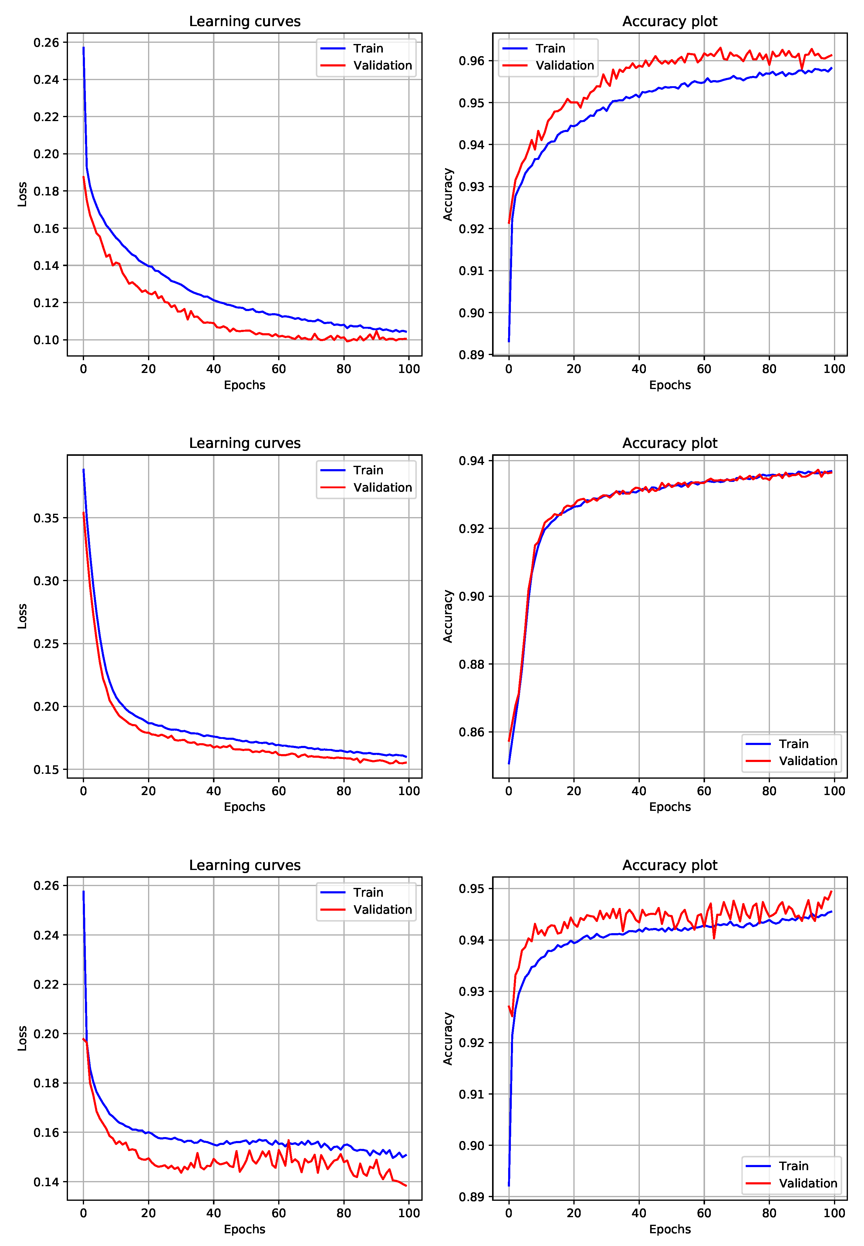
Adam achieved best performance for a 0.001 learning rate and 100 epochs, which is consistent with our previously obtained results. Specifically, this combination reached 96% and 95% Accuracay on the validation and test set, respectively, and 96% AUC on both the validation and test set. Figure 11 visualizes the learning curves on the train and validation set and Accuracy plot with regards to different optimizers for a learning rate of 0.001 and 100 epochs. It can be noticed that, for the Adam optimizer, the Accuracy plot on the Train and Validation set seem to overlap, and the learning curves are almost in a optimal fit.

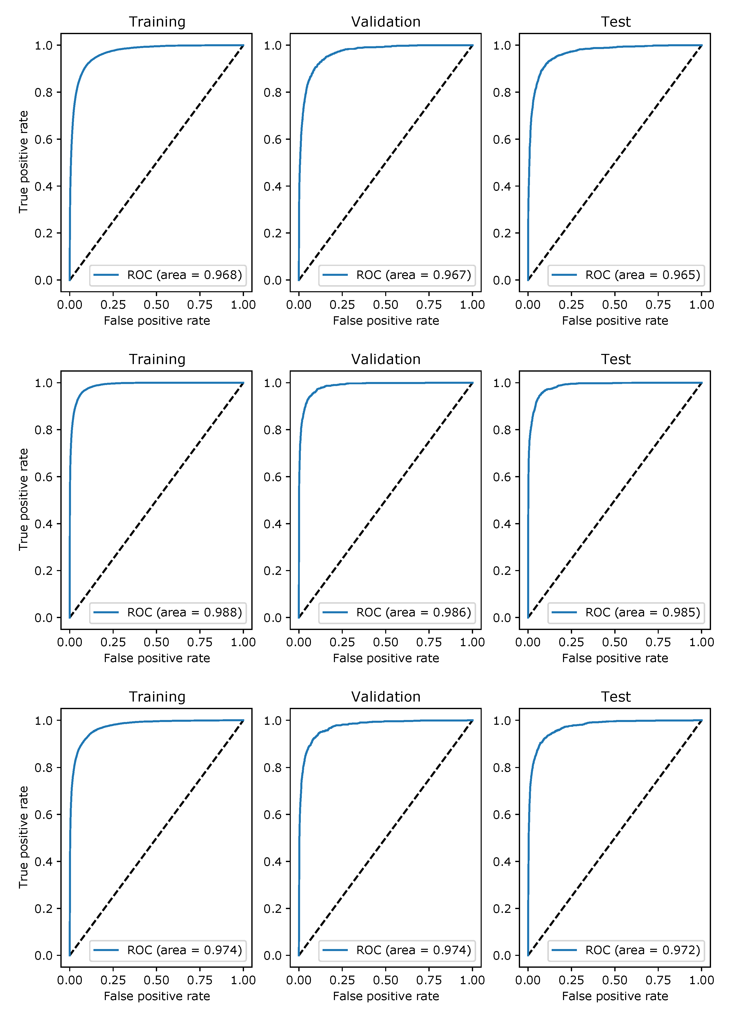
Finally, the performance of the Neural Network as a classifier, for a different combination of optimizers for a learning rate of 0.001 and 100 epochs, is evaluated with the ROC curve visualized in Figure 12. As can be seen, with Adam optimizer, NN as a classifier is able to achieve the highest TPR while maintaining a low FPR. High AUC of 98% implies that the final Neural Network model is able to distinguish occupied and free parking space exceptionally well.

Lastly, we have compared our results with other researches that we have identified in the State of the Art section that have also used Neural Network as a ML technique for the classification or prediction of a free parking space. We have compared them with our results in terms of achieved accuracy and presented the comparison in

Table 11. Comparison table of this paper with other research in terms of accuracy for NN.

Paper	ML Model	Given Accuracy for NN
Vlahogianni et al. [27]	NN (prediction)	0.004 MAE
Farag et al. [28]	NN (classification)	93%
Jones et al. [39]	DT, SVM, k-NN (classification)	81%
Hiesmair et al. [40]	NN, DT, k-NN, SVM (classification)	95% accuracy
Zheng et al. [43]	RT, NN, SVR (prediction)	Mean MAE 0.194–0.059
This paper	HMM, NN (classification)	97% accuracy

.

The researches [27,43] have used Neural Network for future prediction and, therefore, have presented their results in terms of MAE. As can be seen from the table, this paper achieved best performance results in terms of accuracy of NN for classifying a parking space, in comparison to [28,39,40].

8. Conclusions

This paper presents a novel software alternative concept of cost-effective sensor device for parking lot occupancy detection. Namely, a LoRa-based smart parking sensor device measured parking lot occupancy during the period of several months. The parking lot occupancy was sent over a radio channel to three LoRaWAN gateways that collected measurements of signal strength from five sensor devices that were placed on a University parking lot. The analysis of collected data indicates a correlation between RSSI, SNR, and parking lot occupancy. Using related machine learning techniques, it was shown that parking lot occupancy can be estimated from signal strength measurements. Using the Hidden Markov Model with Viterby algorithm and Deep Learning approach based on Neural Networks showed significant results up to 97% of correctly estimating parking lot occupancy. Our future work will comprise an exploration of other ML techniques for parking space classification, which we further plan to evaluate and compare to the results that we have obtained in this paper.