Abstract
In this work, the problem of navigation control of a quad-rotor, which includes path planning (to a desired trajectory with obstacle avoidance) and tracking control, is addressed. Path planning is achieved by means of the velocity field technique, since this method generates smooth trajectories that are suitable for this kind of vehicles. We propose a recursive method for the composition of the total velocity reference. In order to achieve a good tracking of the generated references, a saturated controller is used, namely, nested saturation. It is demonstrated that the velocity reference can be tracked with a reduction in the order of the controller, from four to three saturators, which simplifies the implementation. Numerical results show that a correct tracking could be guaranteed.
1. Introduction
One of the inherent issues in the control of autonomous vehicles is the navigation control, which includes path planning and tracking control [1]. The velocity field could be seen as a stream that drags a vehicle in the direction of that stream at each point. The potential functions are used to generate trajectories and avoid obstacles. The velocity potential functions, obtained from hybrid potential field (HPF), have the advantage of completely eliminating local minima [2]. The velocity field method is attractive because it presents a very low computation cost [3] and is mathematically elegant [2].
Several applications have been proposed using this method. In Reference [4] this technique is used to control multiple three-wheeled robots that cooperate to achieve a task. The use of probabilistic algorithms altogether with the velocity field is developed in Reference [5] where the fuzzy logic defines the velocity to be used in the tracking control. Another application is to generate a trajectory for an unmanned aerial vehicle (UAV) to collect information from a terrain after a natural disaster [6]. In Reference [7] the velocity field is utilized for the movements of an exoskeleton. Recent work in References [8,9,10] uses velocity fields or potential fields, not necessarily to generate strictly a desired path, but for collision avoidance in the path of autonomous vehicles.
The method of velocity field for path planning arose in the early 1990s [11]. Kim and Khosla [2] proposed that this control strategy could be used for real-time control of mobile robots and manipulators. However they just presented numerical results without a dynamic model of a robot. For the purpose of a real path following, an alternative was proposed by P. Y. Li and R. Horowitz [12]; they used a vector field to define a trajectory, thus by tracking the velocity field it is possible to reach the objective. The use of velocity fields for tracking control is considered due to this technique depends on the actual position of the robot, unlike the traditional method which depends on time. The philosophy of this approach is that the robot reaches the velocity defined by the vector field, thus, in that instant the robot will be in the desired trajectory. Some advantages of this method compared to the traditional tracking control, according to [13], are:
- The velocity field error is a more appropriate way to determine whether the contour is being followed or not.
- The specification of the task, encoded as vector field, and the speed at which the task is performed can be decoupled.
- The coordination aspect of the task is explicit.
Masoud [1] mentions that the reference velocity generated with HPF is followed correctly with a massless, single integrator, holonomic system, but not with a more complex system like holonomic vehicles. In order to overcome this problem, he proposes the concept of virtual velocity attractor (VVA) to successfully execute any guidance instruction to drive an UAV closer to its goal. In our work, we propose using an asymptotically stable tracking control in order to track the velocity reference generated by the velocity field. This tracking control takes the velocity error and its derivatives to zero.
Autonomous vehicles like wheeled mobile robots or fixed wing UAVs have non-holonomic constraints; then, with this kind of vehicle the velocity reference is reached by controlling the steering angle, like in References [3,8]. In this paper we use a quad-rotor that can be controlled with decoupled dynamics for pitch and roll, thus, we decompose the velocity vector in x and y components, rather than magnitude of velocity and steering angle.
Recent works [14,15,16] deal with the problem of a UAV tracking a trajectory, like a line or a circular orbit, generated by the vector field method, considering uncertainties associated with modeling errors and compensating for wind uncertainty. Nevertheless, the proposed methods neglect the presence of obstacles. In this work, we propose a trajectory generation using a velocity field similar in the definition of the attractive and evasive field to the one presented in Reference [17]. One fundamental difference is that in Reference [17], the evasive field is added or overlapped, to the global velocity field through a weighted sum of the evasive function to any obstacle. Instead, we propose a strategy, in which each evasive field modifies the previous computed field recursively. Thus the successive derivatives of the desired velocity (references for tracking control) are computed over the last resulting field in a computational recursive way.
Once the velocity field is computed, the vehicle has to track the desired velocity. In order to accomplish a perfect tracking of the velocity field, we used a nested saturation controller [18]. This control law has been proved to be asymptotically stable in regulation and tracking control [19]. Patrikar et al. [20] used the nested saturation method for guidance of UAVs tracking in a circular or elliptical trajectory; however, their work does not considered obstacles avoidance. Tran et al. [21] used nested saturations for quad-rotor trajectory tracking, also neglecting obstacle avoidance. Tran mentions that for the tracking problem it is necessary to track the reference position and its time derivative up to the fourth order. Since the objective of the controller is to track the velocity reference, in our work, we omitted the last saturation term of the nested saturation controller, that corresponds to position, reducing the order of the controller with similar results. Thus demonstrating that, in the case of tracking a velocity reference, our proposed implementation of a nested saturation controller can be simpler than in the complete form, also reducing the computational cost. The tracking form of this controller acts over the velocity error and its successive derivatives; in this case, three successive derivatives of the velocity reference must be computed. We show how to carry out the time derivative of those variables.
This document is organized as follows: in Section 2 we describe the dynamic model of a quad-rotor aerial vehicle; in Section 3 the control strategy for tracking a velocity reference is developed; in Section 4 the velocity field generation is explained; in Section 5 the hydrodynamic theory is used to develop the velocity components which will help us to achieve the obstacle avoidance. The results are shown in Section 6, while conclusions are given in Section 7. Two Appendix A and Appendix B—are included to illustrate the steps required to derive the equations for successive derivatives of attractive and evasive fields.
2. Dynamic Model
The dynamic model of the quad-rotor is obtained, representing the vehicle as a rigid body in a three-dimensional space and attached to one force and three torques. The motors dynamics and propellers flexibility are neglected [22].
Consider a quad-rotor aircraft configuration such as the one shown in Figure 1. The generalized coordinates are
 where denotes the quad-rotor center of mass position, relative to the inertial frame , and represents the orientation vector of the body frame, expressed in Euler’s angles.
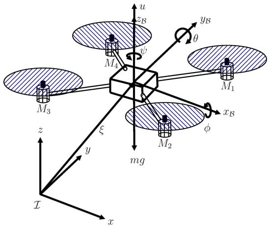
Figure 1.
Quad-rotor frames and generalized coordinates.
The dynamic model of the quad-rotor is given as:
where m stands for the mass of the vehicle, g is the gravitational constant, , , and
where is a vector with the quad-rotor torques, is a vector with the control inputs, represents the inertial matrix and denotes the Coriolis matrix.
The inputs of force and torques, u and , respectively, are related with the velocity of the four rotors as follows. The thrust input, u, is the sum of the thrust of each rotor, expressed by
with
where is a constant coefficient and denotes the angular velocity of the i-th rotor.
The torque inputs , are obtained through
where ℓ is the distance from the rotors to the center of gravity of the quad-rotor, and denotes the gyroscopic torque produced by the motor . The torques are obtained from
where is a constant coefficient. In general, .
3. Control Strategy
For the aircraft control, we assume that the altitude and yaw angle are fixed at some desired value.
3.1. Altitude and Yaw Control
Let us define , such that the quad-rotor maintains a zero degree yaw angle during the flight. The control is obtained through
where , and denote the proportional and derivative constants of the PD controller, respectively.
In a similar way, the control law for maintaining a constant altitude can be achieved by applying the control input
where represents the altitude error, and are positive constants related to the PD controller. The roll and pitch angles () must be small to avoid singularities in (8) and to handle them in the linear region. The nested saturation controller allows that these angles will remain small.
3.2. Roll and Pitch Control
For tracking a trajectory, the nested saturation controller is used. This method was proposed by Teel [18]. It is used to stabilize a chain of integrators in cascade and is asymptotically stable for both, regulation and tracking trajectory. In tracking mode, the nested saturation controller allows to reach high speeds of the vehicle while maintaining bounded control inputs, inside the limits of actuator constraints.
Consider the quad-rotor model (1)–(6), under the control inputs (7) and (8). After a finite time, , and , then, and the system (1)–(6) can be represented as:
and considered to be restricted to small angles and , such that and , and so for , the system (9)–(10) can be seen as a reduced system:
where both subsystems are integrators in cascade
and
Let us define the state variables of each subsystem as and , thereby
With the purpose to achieve the tracking of the trajectory, it is necessary to apply the control over the error vectors, this is
Given that this system will follow a velocity field, the position error could be neglected of the state error vector, and still follow the desired trajectory, so the error vector could be expressed by
Each subsystem can be represented in the form , as in Equation (13), with state vector as in (16), , then a linear transformation exist that maps (13) in , where
where the elements .
In this particular case the transformation matrix elements in matrix are
with the vector of the Equation(16). Given that the state variable is set to 0, the element (1, 1) of matrix can be 0, then
In a similar way , is defined as:
with the vector given in Equation (16), where the control law according to the conventional nested saturation function, for the case of tracking trajectory is
with
where b is a positive constant; therefore, the controller for the pitch angle is
and for the roll angle is
with and as the bounds of the saturation functions.
Since the objective of the vehicle is to follow the desired trajectory according to a velocity field, the error vector (16) could be reduced to
With the new state error vectors (21) instead (16), it is possible to omit the state in the diffeomorphism , then of Equation (17), and in the same way , could be reduced to a matrix
Consequently, the saturation controller (19), could be reduced to only 3 saturators, as:
and for the roll angle:
The control law of three saturators of Equation (23) is equivalent to the control law of Equation (19) with . According to Reference [19], if none of the are saturated, the poles of the linearized closed loop system reside at . This means that in the case of the three saturations controller (23), when none of the are saturated, the poles of the linearized closed loop system reside at . Both controllers are stable; however, the difference between or , going to the same reference, (and in general for every constant ) is that for higher , the error rates in saturated equilibrium decrease, but the overall settling time can be higher.
4. Velocity Field
The objective of the velocity field method in this particular case is to follow a predefined trajectory. For this method, it is necessary to calculate two vector fields, the approaching field and the tangential field. The approaching field is defined by the vectors that aim directly to the trajectory, in which each vector is obtained as the normalized subtraction of the closest point to the trajectory, as proposed by Reference [17]. The trajectory to follow is a circle of radius and the center at the point , expressed by
In order to calculate the approaching field, it is necessary to find the closest point from any position of the workspace to the trajectory. This closest point is calculated by
where and are the points conforming the trajectory, that is, the set of all the points that satisfy Equation (25). For this specific case, let us define the vectors:
where are the difference between any point of the workspace and the center of the circular trajectory, and are the position errors from any point of the workspace and its closest point within the desired trajectory.
The coordinates of the closest point to the trajectory are
where denotes the angle from the actual position to the closest point of the trajectory. Taking the Equations (28)–(29) to calculate and , we can define the distance between the actual position and the closest point in the trajectory as
The angle is obtained from the derivative of the distance with respect to , or , and it is
The approaching field is defined as
Let us denote the partial derivatives of and as and .
These values are necessary to generate the tangential field as follows
The velocity field is obtained performing the normalized weighted sum
where and are functions of the Euclidean distance between a point in space and the desired trajectory, which are given by:
The aim of this function is to increase the effect of the approaching function far from the trajectory and the tangential function close to the trajectory, with as the parameter that controls the weighting of both vectors. In Figure 2 is shown a velocity field generated with a value , , and .
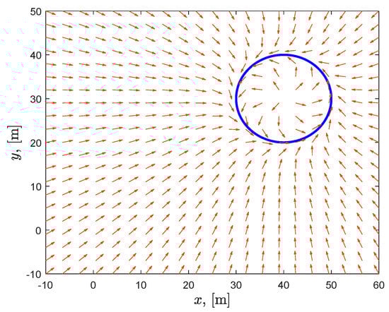
Figure 2.
Velocity field of Equation (35), with desired trajectory at position and radio m.
The velocity field vector is expressed by (35). It represents the desired velocity that the vehicle must achieve at each instant, in order to track the trajectory. With the nested saturation controller, given by Equations (23) and (24), it is possible to track the vectors and given in (21).
Since the velocity field vector (35) is a normalized vector, then the magnitude of the velocity vector is one. In order to impose other magnitude to the velocity reference, this vector could be multiplied by a constant . The resulting vector could be seen as the desired value of the velocity in x and y coordinates, this is:
with these desired values, the velocity error variables and can be computed. However, in order to compute the remaining error variables of Equation (21), are still necessary the desired values: and , even more, the tracking controllers (23) and (24) need the desired variables and . From Equations (13) and (14) we have that and , so and , then
and
Equation (38) gives us a way to obtain the desired variables to track, and it means that it is necessary to compute three successive derivatives of the potential velocity (35). Appendix A illustrates the procedure to obtain the successive derivatives of .
5. Obstacle Avoidance
Obstacle avoidance is achieved by using hydrodynamic theory, specifically the flux of an ideal fluid around a cylinder as shown in Figure 3. Let us define a flux of a planar fluid in stationary state, with a vector velocity field
in the point
Here is the domain occupied by the fluid, then for it to be an ideal fluid it must be incompressible, meaning vanishing divergence, and irrotational, implying a vanishing curl
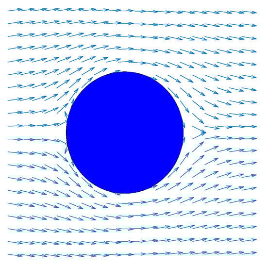
Figure 3.
Flux around a cylinder.
Theorem 1.
The velocity vector field induces a flux of ideal fluid if and only if
is a complex analytic function of [23].
Thus, the components and are necessarily harmonic conjugates. The corresponding complex function (40) is known as the complex velocity of the fluid flux.
Let allow a complex anti-derivative, that is, a complex analytic function
Using the Cauchy-Riemann equations for the complex derivative,
Thus, , and therefore the real part of the complex function defines the velocity potential. Consequently, is known as the complex potential function for the fluid velocity field.
Taking advantage of this property, it is possible to use any harmonic function for the complex velocity potential and the real velocity of the fluid, , is automatically irrotational and incompressible.
Using a circular obstacle that interferes with the approaching vector field flux, where () is the center position of the obstacle, with radius , the position error with respect to the center of the obstacle is defined as
The proposed velocity potential function for an ideal fluid through a circular obstacle is
where
is the angle of the velocity field vector in that point. The flux velocity around a cylinder is defined as the gradient of the function, namely .
Then, the x-component of the velocity vector is
where and . The velocity function in the y-coordinate is
Therefore, the velocity vector for the evasive maneuver is
It could be said that the effect of the equations for evasion is to reorient the direction of the velocity vector, which was computed before considering the obstacle, redirecting the velocity reference to try to surround the obstacle. Then, it makes sense that the modified velocity field, , takes the place of the previous velocity field, however, it could be also normalized as
Appendix B illustrates the procedure to obtain the successive derivatives of the velocity reference , obtained from Equation (45). These derivatives are necessary for tracking control.
Remark 1.
The method proposed to avoid obstacles allows to manage the evasive field for multiple obstacles in a recursive way. In the case of multiple obstacles, the algorithm starts from the attractive velocity field of Equation (35). The next step is to create a list of the obstacles located in the workspace, from the furthest to the closest to the vehicle. Then, considering sequentially all the obstacles, at each iteration, the previous velocity vector is transformed, through Equation (45), in the new velocity field (considering evasion of the k-obstacle), and it will become the new reference of velocity, , in the next iteration. After finishing all iterations, the modified velocity field achieved, becomes the actual velocity reference for Equations (38) and (39).
Figure 4 shows the modification of the velocity field shown in Figure 2, resulting from the incorporation of three obstacles.
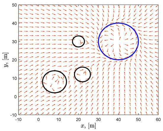
Figure 4.
Velocity field with evasion for three obstacles.
6. Results
6.1. Numerical Results
The first simulation consists only of the approaching velocity field of Equation (35). The vehicle begins at position . In Table 1 are shown the values of the controller parameters for simulation.

Table 1.
Parameters and their corresponding values used in the simulation.
Figure 5 shows the trajectory followed by the vehicle. The “×” symbol points out the initial position, then the vehicle is guided by the velocity field to the circular trajectory.
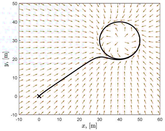
Figure 5.
Quad-rotor trajectory without obstacles.
Figure 6 shows two plots—one for the position error, this is of Equation (27), and the other one for the speed error, this is , where and are defined in Equation (15). It can be seen that the velocity field is reached after 6 seconds, then the vehicle keeps tracking the velocity field thereafter. An adequate tracking of the velocity field leads the vehicle to follow the circular trajectory which is reached around 25 seconds, according to the position error plot, and the vehicle remains in the circular trajectory thereafter at a speed of 2 m/s, according to the selected value for the constant (see Table 1).
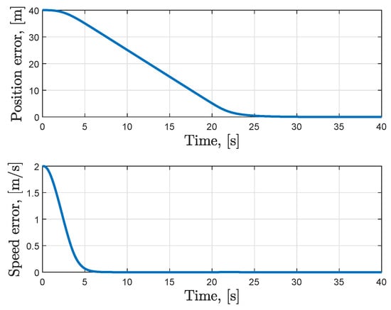
Figure 6.
Position error and velocity error of the simulation without obstacles.
6.2. Obstacle Avoidance Strategy
Figure 7 depicts the trajectory followed by the vehicle in the presence of three obstacles. The “×” symbol shows the initial position. It is shown how the vehicle avoids the obstacles guided by the evasive velocity field.
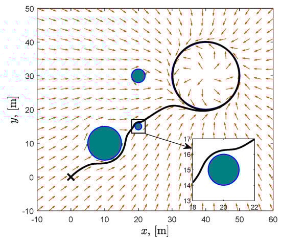
Figure 7.
Quad-rotor trajectory in the presence of obstacles.
Figure 8 illustrates two plots—one for the position error, this is of Equation (27), and the other one for the speed error, this is . It can be seen that the vehicle reaches the velocity field and the desired trajectory almost at the same time of the simulation without obstacles, however, in this case, it could be seen two little humps in the speed error plot. The greater hump (up to 0.03 m/s) occurs around 16.5 s and the other one around 18 s; this occurs after the evasion of the second obstacle.
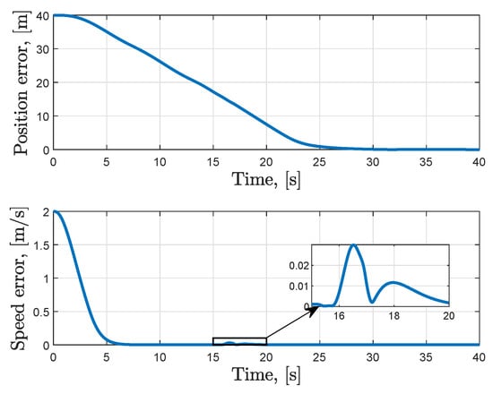
Figure 8.
Position error and velocity error in the presence of obstacles.
6.3. Experimental Results
For the experiments, a 3DR IRIS+ quad-copter was used. This vehicle has a Pixhawk autopilot, and the position was measured with a GPS. The experiment consist in the flight from the point , to the circular reference trajectory with center at the point , and radio = 3 m. One obstacle of radio = 1.5 m was virtually positioned in the coordinate . The Figure 9 shows the path followed by the quad-rotor. The vehicle completed the task satisfactorily and it showed an acceptable performance.
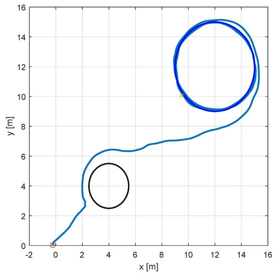
Figure 9.
Quad-rotor flight with virtual obstacle in the x-y plane.
In this experimental test, the obstacle is virtual. However, real obstacles could be detected with multiple sensors like cameras on board the UAV, fixed cameras like those for motion capture, or other sensors like LIDAR. Whatever means of detection is selected, it must be ensured to provide accurate information of the width of the obstacles, to calculate the radius of the cylinder to evade.
7. Conclusions
The most important contributions of this work are: (i) the recursive generation of a velocity field that includes attractive field and evasive field for obstacle avoidance; (ii) the derivation of the time derivatives of the attractive and evasive velocity reference, needed to compute the desired tracking variables; and (iii) the use of a reduced asymptotically stable tracking control law (from four to three saturators), which results simpler for implementation. Simulation results show that the tracking nested saturation controller for velocity vanishes the velocity error and its derivatives, which indicate that the velocity field is perfectly tracked, showing that the combination of these strategies provides a reasonable tracking performance.
For future work, we will consider obstacles with arbitrary shapes by using the panel method. Also, a robust control for wind perturbations will be considered.
Author Contributions
In this paper, conceptualization, investigation and methodology were performed by J.R.-E., L.A.G.-D., A.G.-J. and J.R.N. Formal analysis and validation were developed by J.R.-E. and E.S.E. The original draft was written by J.R.-E. and L.A.G.-D., while all the authors contributed equally in the review and editing of the manuscript. The project administrator is L.A.G.-D. All authors have read and agree to the published version of the manuscript.
Funding
This work was supported by Universidad de Sonora with internal project USO315005985.
Acknowledgments
We would like to thank CONACyT for the scholarship program, PRODEP for its financial support and UMI-LAFMIA Cinvestav, Zacatenco for their support and guidance in the experimental tests.
Conflicts of Interest
The authors declare no conflict of interest.
Appendix A. Derivative of Velocity field
In order to track the velocity field of Equation (35), with nested saturation controllers of Equations (23) and (24), it is necessary to compute three successive derivatives of the velocity reference (35), according to (38). In this appendix the equations to obtain the first derivative, , of the velocity field are derived.
Appendix A.1. First derivative of velocity field
The derivative of the angle (the angle from the actual position to the closest point of the trajectory, of Equation (31)) is
The time derivative of the points and of Equations (28) and (29) is
where and are those of Equation(33).
The time derivative of the error between the actual position and the closest point of the trajectory, of Equation (27), is
The derivative of the approaching field defined on Equation (32) is
The vector for the derivative of tangential velocity is
Then, the time derivative of tangential field of Equation (34) is
The time derivative of the functions and of Equation (36), is defined as
Thus, the time derivative of the velocity field is
Appendix A.2. Second and Third Derivative of Velocity Field
The derivation of the second and third derivatives implies two successive derivatives of Equations (A1)–(A10). We will just present the second and third derivative of in order to be more concise.
The second derivative of the velocity field is
and the third derivative of this function is
Appendix B. Derivative of Evasive Velocity Field
The evasive velocity field is expressed by Equation (45), which requires the vector of Equation (44). The next subsection shows the derivative of the evasive velocity field (45).
Appendix B.1. First Derivative of Velocity Field
The derivative of the angle , of Equation (41), (the angle of velocity field before the addition of the considered obstacle) is
Appendix B.2. Second and Third Derivative of Evasive Velocity Field
The derivation of the second and third derivatives implies two successive derivatives of Equations (A13)–(A16). The second and third derivative of Equations (42) and (43) results in long equations of many terms. We will just present the second and third derivative of in order to be more concise.
The second derivative of the velocity field is
and the third derivative of this function is
References
- Masoud, A.A. A Harmonic Potential Approach for Simultaneous Planning and Control of a Generic UAV Platform. J. Intell. Robot. Syst. 2012, 65, 153–173. [Google Scholar] [CrossRef]
- Kim, J.; Khosla, P.K. Real-time obstacle avoidance using harmonic potential functions. IEEE Trans. Robot. Autom. 1992, 8, 338–349. [Google Scholar] [CrossRef]
- Shibata, N.; Sugiyama, S.; Wada, T. Collision avoidance control with steering using velocity potential field. In Proceedings of the 2014 IEEE Intelligent Vehicles Symposium Proceedings, Dearborn, MI, USA, 8–11 June 2014; pp. 438–443. [Google Scholar]
- Yamakita, M.; Yazawa, T.; Zheng, X.Z.; Ito, K. An application of Passive Velocity Field Control to cooperative multiple 3-wheeled mobile robots. In Proceedings of the 1998 IEEE/Rsj International Conference on Intelligent Robots and Systems, Victoria, BC, Canada, 17 October 1998; Volume 1–3, pp. 368–373. [Google Scholar]
- Perez-D’Arpino, C.; Medina-Melendez, W.; Guzman, J.; Fermin, L.; Fernandez-Lopez, G. Fuzzy logic based speed planning for autonomous navigation under Velocity Field Control. In Proceedings of the 2009 IEEE International Conference on Mechatronics, Malaga, Spain, 14–17 April 2009; Volume 1, pp. 1–6. [Google Scholar]
- Fukao, T.; Yuzuriha, A.; Suzuki, T.; Kanzawa, T.; Oshibuchi, T.; Osuka, K.; Kohno, T.; Okuyama, M.; Tomoi, Y.; Nakadate, M. Inverse Optimal Velocity Field Control of an Outdoor Blimp Robot—Blimp Surveillance Systems for Rescue. IFAC Proc. Vol. 2008, 41, 4374–4379. [Google Scholar] [CrossRef]
- Asl, H.J.; Narikiyo, T.; Kawanishi, M. Neural Network Velocity Field Control of Robotic Exoskeletons with Bounded Input. In Proceedings of the 2017 IEEE International Conference on Advanced Intelligent Mechatronics (AIM), Munich, Germany, 3–7 July 2017; pp. 1363–1368. [Google Scholar]
- Li, B.; Du, H.; Li, W. A Potential Field Approach-Based Trajectory Control for Autonomous Electric Vehicles With In-Wheel Motors. IEEE Trans. Intell. Transp. Syst. 2017, 18, 2044–2055. [Google Scholar] [CrossRef]
- Wang, T.; Lima, R.M.; Giraldi, L.; Knio, O.M. Trajectory planning for autonomous underwater vehicles in the presence of obstacles and a nonlinear flow field using mixed integer nonlinear programming. Comput. Oper. Res. 2019, 101, 55–75. [Google Scholar] [CrossRef]
- Huang, Y.; Ding, H.; Zhang, Y.; Wang, H.; Cao, D.; Xu, N.; Hu, C. A Motion Planning and Tracking Framework for Autonomous Vehicles Based on Artificial Potential Field-Elaborated Resistance Network (APFE-RN) Approach. IEEE Trans. Ind. Electron. 2019, 67, 1376–1386. [Google Scholar] [CrossRef]
- Connolly, C.I.; Burns, J.B.; Weiss, R. Path planning using Laplace’s equation. In Proceedings of the IEEE International Conference on Robotics and Automation, Cincinnati, OH, USA, 13–18 May 1990; Volume 3, pp. 2102–2106. [Google Scholar]
- Li, P.; Horowitz, R. Passive velocity field control of mechanical manipulators. IEEE Trans. Robot. Autom. 1999, 15, 751–763. [Google Scholar] [CrossRef]
- Cervantes, I.; Kelly, R.; Alvarez-Ramírez, J.; Moreno, J. A Robust Velocity Field Control. Control 2002, 10, 888–894. [Google Scholar] [CrossRef]
- Zhou, B.; Satyavada, H.; Baldi, S. Adaptive path following for Unmanned Aerial Vehicles in time-varying unknown wind environments. In Proceedings of the 2017 American Control Conference (ACC), Seattle, WA, USA, 24–26 May 2017; pp. 1127–1132. [Google Scholar]
- Olavo, J.L.G.; Thums, G.D.; Jesus, T.A.; de Araújo Pimenta, L.C.; Torres, L.A.B.; Palhares, R.M. Robust Guidance Strategy for Target Circulation by Controlled UAV. IEEE Trans. Aerosp. Electron. Syst. 2018, 54, 1415–1431. [Google Scholar] [CrossRef]
- Fari, S.; Wang, X.; Roy, S.; Baldi, S. Addressing Unmodelled Path-Following Dynamics via Adaptive Vector Field: A UAV Test Case. IEEE Trans. Aerosp. Electron. Syst. 2019, 1. [Google Scholar] [CrossRef]
- Pérez-D’Arpino, C.; Medina-Meléndez, W.; Fermín, L.; Guzmán, J.; Fernández-López, G.; Grieco, J.C. Dynamic Velocity Field Angle Generation for Obstacle Avoidance in Mobile Robots Using Hydrodynamics. In Advances in Artificial Intelligence—IBERAMIA 2008; Geffner, H., Prada, R., Machado Alexandre, I., David, N., Eds.; Springer: Berlin/Heidelberg, Germany, 2008; pp. 372–381. [Google Scholar]
- Teel, A.R. Global stabilization and restricted tracking for multiple integrators with bounded controls. Syst. Control. Lett. 1992, 18, 165–171. [Google Scholar] [CrossRef]
- Johnson, E.N.; Kannan, S.K. Nested saturation with guaranteed real poles. In Proceedings of the 2003 American Control Conference, Denver, CO, USA, 4–6 June 2003; Volume 1, pp. 497–502. [Google Scholar]
- Patrikar, J.; Makkapati, V.R.; Pattanaik, A.; Parwana, H.; Kothari, M. Nested Saturation Based Guidance Law for Unmanned Aerial Vehicles1. J. Dyn. Syst. Meas. Control. 2019, 141, 71008. [Google Scholar] [CrossRef]
- Tran, T.T.; Han, T.T.; Ge, S.S. Trajectory Tracking Control of Quadrotor Aerial Vehicle. IFAC Proc. Vol. 2013, 46, 274–279. [Google Scholar] [CrossRef]
- Castillo, P.; Lozano, R.; Dzul, A. Stabilization of a mini-rotorcraft having four rotors. IEEE Control. Syst. Mag. 2005, 25, 45–55. [Google Scholar]
- Olver, P.J. Complex Analysis and Conformal Mapping; Technical report; University of Minnesota: Minneapolis, MN, USA, 2013. [Google Scholar]


© 2020 by the authors. Licensee MDPI, Basel, Switzerland. This article is an open access article distributed under the terms and conditions of the Creative Commons Attribution (CC BY) license (http://creativecommons.org/licenses/by/4.0/).