Method of Moments Based on Equivalent Periodic Problem and FFT with NURBS Surfaces for Analysis of Multilayer Periodic Structures

Abstract

In this paper, an efficient technique of computation of method of moments (MM) matrix entries for multilayer periodic structures with NURBS surface and Bézier patches modelling is proposed. An approximation in terms of constant pulses of generalized rooftop basis functions (BFs) defined on Bézier patches is proposed. This approximation leads discrete convolutions instead of usual continuous convolution between Green’s functions and BFs obtained by the direct mixed potential integral equation (MPIE) approach. An equivalent periodic problem (EPP) which contains the original problem is proposed to transform the discrete convolutions in discrete cyclic convolutions. The resultant discrete cyclic convolutions are computed by efficiently using the Fast Fourier Transform (FFT) procedure. The performance of the proposed method and direct computation of the MM entries are compared for phases of reflection coefficient. The proposed method is between 9 and 50 times faster than the direct computation for phase errors less than 1 deg. The proposed method exhibits a behaviour of CPU time consumption of O(N_bLog10N_b) as the number N_b of BFs increases. This behaviour provides significant CPU time savings with respect to the expected behaviour of O(N_b²) provided by the direct computation of the MM matrix entries.

1. Introduction

In the design and analysis of electromagnetic devices likes frequency selective surfaces (FSSs) [1], reflectarrays/transmitarrays [2], leaky wave antennas [3] and metasurfaces antennas [4], efficient electromagnetic analysis tools of multilayer periodic structures are required. Although reflectarrays/transmitarrays, leaky wave antennas and metasurfaces antennas are not strictly periodic structures, in the design of these antennas, it is common practice to assume that each element of the antenna is located in periodic environment. This is known as the local periodicity assumption [2].

Some popular of numerical tools of periodic structures are based on Finite Element (FE) [5], Finite Difference Time Domain (FDTD) [6] and MM [7], all methods under periodic boundary conditions. Although FE and FDTD are mature methods, these methods involve volumetric meshes to model the multilayer medium which hosts the unit cell of the periodic structure. This volumetric mesh involves a large amount of numerical computations which slow down the electromagnetic analysis. Thus, the MM is preferable because the multilayer medium is modelled by Green’s functions and the volumetric mesh is avoided. The work shown in this paper will be focused in MM formulation for an analysis of multilayer periodic structures. There are recent papers that attempted sophisticated improvements on the MM [8,9,10], also for multilayer periodic structures [11,12,13]. The MM is usually used to solve electric field integral equations (EFIEs) where the unknowns are the induced current densities on the metallic layout. These EFIEs show hypersingular behaviour of the kernel (Green’s functions) which cause difficulties in the solution procedure [14]. This hypersingular behaviour may be avoided if the electric fields are expressed in terms of vector and scalar potentials with weakly singular kernels. This led to the development of MPIEs [15]. In this latter approach, for the case of periodic structures, one has to face with the computation of multilayer periodic Green’s functions consisting of slowly convergent double infinite summations. Fortunately, there are pre-processing techniques to interpolate efficiently the Green’s functions in terms of Chebyshev polynomials after extracting known singular behaviour around the source point [11]. Therefore, this approach involves surface mesh to model the geometry layout hosted in the unit cell of the multilayer periodic structures with accurate computation of the multilayer periodic Green’s functions. Once an accurate computation of multilayer periodic Green’s functions is available, the induced current density on the metallic layout is expanded in terms on BFs weighted by unknown coefficients. When this expansion is taken into account in the MPIEs and a method of weighted residual is applied, a linear system of equations is obtained. The elements of the coefficient matrix of the resultant linear system of equations involve the computation of convolutions between the Green’s function and the BFs used in the expansion of the density current. These convolutions involve the integration of singular behaviour of the integrand introduced by the Green’s function when the observation point and the source point are close. Fortunately, there are direct methods of numerical integration of the singular behaviour of the integrand as double exponential (DE) formulas [16] or Ma-Rokhlin-Wandzura (MRW) quadrature rules [17,18].

On the other hand, in order to provide accurate electromagnetic models of complex geometries of the layout, NURBS surfaces are usually used by computer-aided geometry design (CAGD) tools [19]. NURBS surfaces are quite useful because they provide invariance under rotation, scaling, translation and perspective transformation of control points. Moreover, they allow complex shapes to be defined by means of a small number of NURBS. These NURBS surfaces are efficiently written in terms of piecewise Bézier patches as it is described in [19] using Cox-de Boor transformation algorithm [20]. Bézier patches are parametric surfaces defined by Bernstein polynomials [21,22] and they are suitable for numerical computation of parameters associated with the surface (curvature, derivatives, integrations) thanks to the properties of Bernstein polynomials. Thus, Bézier patches are suitable domains to define known subsectional BFs which approximates the induced density currents on the metallic surface. In fact, generalized subsectional rooftop BFs are defined on a pair of adjacent Bézier patches in [19] to approximate the surface density currents induced on metallic surfaces. Despite all these improvements, the direct computation of MM matrix entries leads to computational complexity of CPU time consumption as a function of the number of BFs N_b which is roughly O(N_b²) [23,24]. This computational complexity is inherent to the direct computation of MM matrix entries because it requires the computation of a MM matrix with dimensions of N_b×N_b element by element.

In [25] and [26], the Conjugate Gradient Fast Fourier Transform (CG-FFT) method is proposed to solve electromagnetic problems. This CG-FFT method uses as BFs rooftops defined on a regular rectangular mesh to expand the current density. The advantage of this approach is that the convolutions between Green’s functions and the BFs are expressed as discrete cyclic convolutions which are computed by FFT algorithm. In this way, the consumption of CPU time involved in the computation of these cyclic convolutions are proportional to N_bLog10(N_b). Thus, the behaviour of CPU time with respect to the number of BFs, N_b, involves important CPU time savings as N_b increases when it is compared to that provided by the direct computation of MM matrix entries. However, this approach has a drawback because it uses regular rectangular meshes. In order to model accurately complex geometries (e.g., geometries with a combination of thin strips and/or patches, patches with curve boundaries, etc.) it needs a very dense mesh. This requires a high number of rooftops to approximate the surface currents which leads to systems of equations with a high number of unknowns.

In other very general formulations for multilayered problems [27,28], Rao-Wilton-Glisson (RWG) BFs [29] defined on triangular surfaces are also approximated in an expansion of pulses. However, this approximation is accurate for sufficient separation of the source and the observation triangular surfaces. Under this condition, the MM matrix entries are computed using a conventional pre-corrected FFT algorithm [30].

In this work, we used generalized rooftop defined over pair of adjacent Bézier patches. These rooftops are approximated in an expansion of pulses with enough dense equi-spaced meshes in order to keep the high-order description of the geometry. Thus, the approach is suitable for complex geometries (geometries with a combination of thin strips and/or patches, patches with curve boundaries, etc.) when very dense equi-spaced meshes are used in the pulse expansion. This approximation leads to discrete convolutions instead of usual continuous convolution between Green’s functions and BFs. Since the Green’s functions and generalized rooftops involved in the discrete convolutions are not strictly periodic functions, an EPP which contains the original problem is proposed [26]. We show that this new approach leads to discrete cyclic convolutions which were be efficiently computed for a very dense equi-spaced mesh by means of an FFT procedure. Since the original problem is contained in the EPP, this approach does not require considering different formulations when the source and the observation points are close or far. Moreover, unlike the CG-FFT method, the increment of density of the equi-spaced mesh does not lead to an increment of number of unknowns.

This paper is organized as follows. Section 2 shows a description of the problem which is faceted by the direct MM using a generalized rooftop defined on a pair of adjacent Bézier patches and ‘razor-blade’ as weighted functions. In this section, the formulation of direct numerical integration involved in the MM matrix entries is shown. Section 3 shows an efficient computation of these matrix entries using the pulse approximation of the generalized rooftop BFs and EPP approach. Section 4 shows an efficient computation of integrals of the Green’s functions in each pulse domain which are required in the formulation described in the previous section. Section 5 shows convergence results and CPU time consumption obtained by the proposed method and by the direct computation of the MM matrix entries. Validations of both numerical techniques are also shown with different periodic structures. Finally, the conclusions are provided in Section 6.

2. Description of the Problem

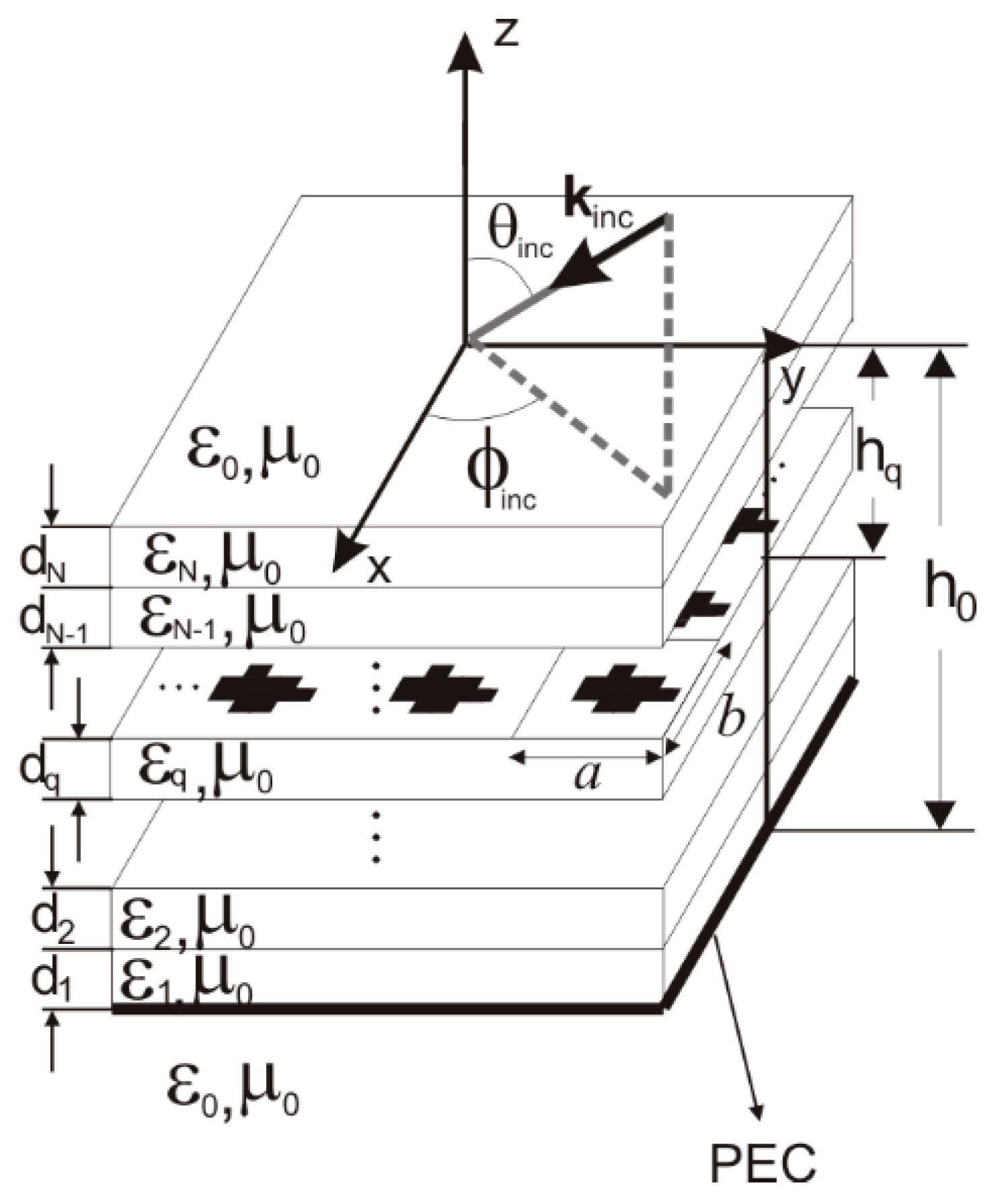
Figure 1 shows a multilayer periodic structure. The patches are assumed to be PEC with negligible thickness. The multilayer substrate consists of N lossy dielectric layers with thickness d_k and complex permittivity ε_k= ε₀ε_r,k(1-jtanδ_k) (k=1,…,N). The lower limit of the multilayer substrate is a ground plane. The qth-interface hosts a periodical array of patches with arbitrary geometry. In order to simplify the notation, we show a formulation with unique interface which hosts a periodical array of patches. The formulation can be easily extended with more interfaces with periodical structures. The periodic structure of Figure 1 is illuminated by a linearly polarized plane wave with an arbitrary polarization direction and the incidence direction is given by the angular spherical coordinate θ_inc and ϕ_inc. A time dependence of the type e^jωt is assumed and this dependence is suppressed throughout. In order to determine the electric field scattered by the periodic structure of Figure 1, we need to determine the induced surface current densities J(x,y) hosted on the unit cell of the qth-interface of the periodic array of patches. These surface current densities can be obtained by solving MPIE [15]:

$$\begin{array}{l}{E}_t^{\mathrm{exc}}(x,y,z=-h_{\mathrm{q}})-j\omega {\displaystyle \underset{S}{\int }{G}_{xx}^{\mathrm{A}}(x-x^{\prime },y-y^{\prime },z=-h_{\mathrm{q}},z^{\prime }=-h_{\mathrm{q}})J(x^{\prime },y^{\prime })d{x}^{\prime }d{y}^{\prime }}\\ -\nabla {\displaystyle \underset{S}{\int }{G}^{\Phi }(x-x^{\prime },y-y^{\prime },z=-h_{\mathrm{q}},z^{\prime }=-h_{\mathrm{q}})\sigma (x^{\prime },y^{\prime })d{x}^{\prime }d{y}^{\prime }=0}\end{array}$$

(1)

where E_t^exc(x,y,z=-h_q) is the tangential electric field generated in the observation point (x,y,z=-h_q) by the plane wave impinging on the multilayer substrate in the absence of the patches. G^A_xx and G^Φ are the periodic Green’s functions for the x-component of the vector potential and the scalar potential, respectively, of the multilayer substrate of Figure 1. σ is the surface charge density induced on the surface S of the patch hosted in the unit cell of the periodic array of patches of the qth-interface. The induced surface charge density σ is related with the induced surface current density J by the known continuity equation:

$$\sigma (x^{\prime },y^{\prime })=-\frac{1}{j\omega }{\nabla }^{\prime }J(x^{\prime },y^{\prime })$$

(2)

Note that gradient operators work on prime variables x’ and y’ of the source point on the surfaces of patches. We would like to point out that in this work, the periodic Green’s function of the multilayer substrate for the x-component of the vector potential G^A_xx and for the scalar potential G^Φ were efficiently obtained by the pre-processing procedure of interpolation described in [11]. In this procedure, the periodic Green’s functions of the multilayer substrate are judiciously interpolated in the spatial domain in terms of 2-D Chebyshev polynomials after extracting the singular behaviour of the Green’s functions around the source points (which includes the source singularities plus the images through the closest layers). If the MM is used to solve the MPIE shown in Equation (1), J(x,y) would have to be expanded in terms of known BFs J_j(x,y) (j=1,…,N_b), as shown below:

$$J(x^{\prime },y^{\prime })={\displaystyle \sum _{\mathrm{j}=1}^{{\mathrm{N}}_{\mathrm{b}}}{c}_{\mathrm{j},}{J}_{\mathrm{j}}(x^{\prime },y^{\prime })};{\sigma }_{\mathrm{j}}(x^{\prime },y^{\prime })=-\frac{1}{j\omega }{\nabla }^{\prime }{J}_{\mathrm{j}}(x^{\prime },y^{\prime })$$

(3)

Since the surface charge densities and current densities are related by the continuity Equation (2), the BF for the surface charge densities σ_j(x,y) are related with the BF for the current densities J_j(x,y) in similar way as shown in Equation (3). In this paper, the surface of the metallic layout hosted in the unit cell of the qth-interface is modelled by NURBS surfaces. These NURBS surfaces are efficiently written in terms of piecewise Bézier patches as is described in [19] using the Cox-de Boor transformation algorithm [20]. Thus, the BFs J_j(x,y) (j=1,…,N_b) used in this paper are generalized “rooftop” functions defined on pairs of adjacent Bézier patches that share a common boundary line, as described in [19]. According to [19], the BF σ_j(x,y) is constant in each Bézier patch.

In order to solve the MPIE given in Equation (1), the method of weighted residual was carried out using “razor-blade” as the weighting function. These “razor-blades” are defined in the qth-interface over the isoparametric curved lines C_i. This curved line joins the centres of the pair of adjacent Bézier patches associated to each BF J_j(x,y) (see [19]). Thus, when Equation (3) is introduced into Equation (1) and “razor-blade” functions are used, the following system of linear equations for the unknown coefficients c_j is obtained:

$${\displaystyle \sum _{\mathrm{j}=1}^{{\mathrm{N}}_{\mathrm{b}}}{Z}_{\mathrm{ij}}{c}_{\mathrm{j}}=e_{\mathrm{i}}}(\mathrm{i}=1,\dots ,{\mathrm{N}}_{\mathrm{b}})$$

(4)

where the coefficients e_i of the system of the linear equations can be computed by the next line integral:

$$e_{\mathrm{i}}={\displaystyle \underset{C_{\mathrm{i}}}{\int }{E}_t^{\mathrm{exc}}(x,y,z=-h_{\mathrm{q}})\cdot dr}$$

(5)

The elements of the coefficient matrix of the system of linear equations of (4) can be broken down in inductive and capacitive contribution:

$$Z_{\mathrm{ij}}=Z_{\mathrm{ij}}^{\mathrm{ind}}+Z_{\mathrm{ij}}^{\mathrm{cap}}$$

(6)

where the inductive contribution of each element of the coefficient matrix is given in terms of the line integral of the bi-dimensional convolutions between periodic Green’s function G^A_xx for the x-component of the vector potential and the BF J_j(x,y), as shown in Equation (7). These bi-dimensional convolutions involve the integration of singular behaviour of the integrand introduced by the periodic Green’s function when the observation point (x,y,z=-h_q) and source point (x’,y’,z’=-h_q) are close.

$$Z_{\mathrm{ij}}^{\mathrm{ind}}=j\omega {\displaystyle \underset{C_{\mathrm{i}}}{\int }\left[{\displaystyle \underset{S_{\mathrm{j}}}{\int }{G}_{xx}^{\mathrm{A}}(x-x^{\prime },y-y^{\prime },z=-h_{\mathrm{q}},z^{\prime }=-h_{\mathrm{q}})J_{\mathrm{j}}(x^{\prime },y^{\prime })d{x}^{\prime }d{y}^{\prime }}\right]\cdot dr}$$

(7)

The numerical integration of the singular behaviour of the integrand can be accurately computed by DE formulas [16] or MRW quadrature rules [17,18]. On the other hand, the capacitive contribution is given by the line integral of the gradient of the bi-dimensional convolution between periodic Green’s function G^Φ for scalar potential and the BF σ_j(x,y). Since the capacitive contribution involves a line integral whose integrand is an exact differential, this line integral can be analytically expressed as the difference of bi-dimensional convolutions, as shown in Equation (8). According to [19], the observation points (x⁺_i, y⁺_i, -h_q) and (x^-_i, y^-_i, -h_q) are the centres of the pair of adjacent Bézier patches associated to BF σ_j(x,y) (i.e., the extremes points of the isoparametric curved lines C_i).

$$\begin{array}{l}{Z}_{\mathrm{ij}}^{\mathrm{cap}}=[{\displaystyle \underset{S_{\mathrm{j}}}{\int }{G}^{\Phi }(x_{\mathrm{i}}^{+}-x^{\prime },y_{\mathrm{i}}^{+}-y^{\prime },z=-h_{\mathrm{q}},z^{\prime }=-h_{\mathrm{q}}){\sigma }_{\mathrm{j}}(x^{\prime },y^{\prime })d{x}^{\prime }d{y}^{\prime }}-\\ -{\displaystyle \underset{S_{\mathrm{j}}}{\int }{G}^{\Phi }(x_{\mathrm{i}}^{-}-x^{\prime },y_{\mathrm{i}}^{-}-y^{\prime },z=-h_{\mathrm{q}},z^{\prime }=-h_{\mathrm{q}}){\sigma }_{\mathrm{j}}(x^{\prime },y^{\prime })d{x}^{\prime }d{y}^{\prime }}]\end{array}$$

(8)

Again, the bi-dimensional convolutions involve the integration of singular behaviour which can be accurately computed by DE formulas [16] or MRW quadrature rules [17,18].

The main drawback of the direct computation of the inductive and capacitive contributions of the coefficient matrix given in Equations (7) and (8) is that the CPU time consumption is proportional to the size of the coefficient matrix of the linear system of equations (i.e., the computational complexity of CPU time consumption as a function of the number of unknown N_b is roughly O(N_b²)) [23,24]. Thus, if a very high number N_b of the BFs is required for the approximation of the induced surface density current on the patches, the required CPU time consumption involved in the computation of all elements of coefficient matrix may be prohibitive. In the next section, we describe a procedure for the computation of the inductive and capacitive contributions which involves the FFT algorithm. This approach does not require considering the different formulations when the source and the observation points are close or far, as is required in [27,28]. This procedure provides significant CPU time saving and behaviour of CPU time consumption of O(N_bLog₁₀N_b) as N_b increases, as will be shown in the following sections.

3. Efficient Computation of MM Matrix Entries Using Pulses Expansions of BFs

In the previous section, the induced surface current J(x,y) and charge σ(x,y) density are expanded in terms of known BFs J_j(x,y) and σ_j(x,y) (j=1,…,N_b) to solve the MPIE given in Equation (1). These BFs can be expanded in terms of pulses as shown below:

$$J_{\mathrm{j}}(x^{\prime },y^{\prime })\approx {\displaystyle \sum _{m^{\prime }=0}^{2N_x+1}{\displaystyle \sum _{n^{\prime }=0}^{2N_y+1}{J}_{\mathrm{j}}(x_{m^{\prime }},y_{n^{\prime }})P(x^{\prime }-x_{m^{\prime }},y^{\prime }-y_{n^{\prime }})}}$$

(9)

$${\sigma }_{\mathrm{j}}(x^{\prime },y^{\prime })\approx {\displaystyle \sum _{m^{\prime }=0}^{2N_x+1}{\displaystyle \sum _{n^{\prime }=0}^{2N_y+1}{\sigma }_{\mathrm{j}}(x_{m^{\prime }},y_{n^{\prime }})P(x^{\prime }-x_{m^{\prime }},y^{\prime }-y_{n^{\prime }})}}$$

(10)

where x_m’=x₀+m’Δx, y_n’=y₀+n’Δy are equi-spaced mesh points and P(·) is the pulse function defined as

$$P(x,y)=\{\begin{array}{cc}1& \mathrm{if}\left|x\right|<\frac{\Delta x}{2}\mathrm{and}\left|y\right|<\frac{\Delta y}{2}\\ 0& \mathrm{elsewhere}\end{array}$$

(11)

The expansions given in Equations (9) and (10) approximate the values of the BF J_j(x’,y’) and σ_j(x’,y’) as the constant values J_j(x_m’,y_n’) and σ_j(x_m’,y_n’), respectively, in the intervals x_m’-Δx/2<x’<x_m’+Δx/2 and y_n’-Δy/2<y’<y_n’+Δy/2. Thus, the pulse approximation of the BF improves as the density of the equi-spaced mesh increases (i.e., the values of N_x and N_y of the upper limit of the expansion increase as the values of Δx and Δy decrease). We would like to point out that the BFs are defined on pair of adjacent Bézier patches associated with NURBS surfaces. Thus, the BFs are capable of taking into account a high-order description of the geometry of layout hosted by the unit cell. Since these same BFs are expanded in terms of pulses with very dense equi-spaced meshes, the high-order description of the geometry is kept.

When Equations (9) and (10) are introduced into Equations (7) and (8), the following inductive and capacitive contributions of the coefficients matrix are obtained:

$$Z_{\mathrm{ij}}^{\mathrm{ind}}=j\omega {\displaystyle \underset{C_{\mathrm{i}}}{\int }{f}_{\mathrm{j}}^{\mathrm{ind}}(x,y,z=-h_{\mathrm{q}})\cdot dr}$$

(12)

$$Z_{\mathrm{ij}}^{\mathrm{cap}}=[f_{\mathrm{j}}^{\mathrm{cap}}(x_{\mathrm{i}}^{+},y_{\mathrm{i}}^{+},z=-h_{\mathrm{q}})-f_{\mathrm{j}}^{\mathrm{cap}}(x_{\mathrm{i}}^{-},y_{\mathrm{i}}^{-},z=-h_{\mathrm{q}})]$$

(13)

where

$$f_{\mathrm{j}}^{\mathrm{ind}}(x,y,z)={\displaystyle \sum _{m^{\prime }=0}^{2N_x+1}{\displaystyle \sum _{n^{\prime }=0}^{2N_y+1}{J}_{\mathrm{j}}(x_{m^{\prime }},y_{n^{\prime }})G_{m^{\prime },n^{\prime }}^{\mathrm{A}}(x,y,z)}}$$

(14)

$$f_{\mathrm{j}}^{\mathrm{cap}}(x,y,z)={\displaystyle \sum _{m^{\prime }=0}^{2N_x+1}{\displaystyle \sum _{n^{\prime }=0}^{2N_y+1}{\sigma }_{\mathrm{j}}(x_{m^{\prime }},y_{n^{\prime }})G_{m^{\prime },n^{\prime }}^{\Phi }(x,y,z)}}$$

(15)

and

$$G_{m^{\prime },n^{\prime }}^{\mathrm{A}}(x,y,z)={\displaystyle \underset{m^{\prime }\Delta x-\frac{\Delta x}{2}}{\overset{m^{\prime }\Delta x+\frac{\Delta x}{2}}{\int }}{\displaystyle \underset{n^{\prime }\Delta y-\frac{\Delta y}{2}}{\overset{n^{\prime }\Delta y+\frac{\Delta y}{2}}{\int }}{G}_{xx}^{\mathrm{A}}(x-x^{\prime },y-y^{\prime },z,z^{\prime }=-h_{\mathrm{q}})d{x}^{\prime }d{y}^{\prime }}}$$

(16)

$$G_{m^{\prime },n^{\prime }}^{\Phi }(x,y,z)={\displaystyle \underset{m^{\prime }\Delta x-\frac{\Delta x}{2}}{\overset{m^{\prime }\Delta x+\frac{\Delta x}{2}}{\int }}{\displaystyle \underset{n^{\prime }\Delta y-\frac{\Delta y}{2}}{\overset{n^{\prime }\Delta y+\frac{\Delta y}{2}}{\int }}{G}^{\Phi }(x-x^{\prime },y-y^{\prime },z,z^{\prime }=-h_{\mathrm{q}})d{x}^{\prime }d{y}^{\prime }}}$$

(17)

The direct evaluation of the inductive and capacitive contributions given in Equations (12) and (13) involves the summation of double series Equations (14) and (15) whose addends involve double integrals given by Equations (16) and (17). Moreover, these double series have a high number of addends since a high density of the equi-spaced mesh is required in order to provide accurate approximation of the BFs in terms of pulses. Thus, this approach may seem inappropriate. Let us define the following discrete functions for the BF of the surface current and charge densities:

$$J_{\mathrm{j},x/y}^{\mathrm{d}}[m^{\prime },n^{\prime }]=J_{\mathrm{j},x/y}(x_{m^{\prime }},y_{n^{\prime }})$$

(18)

$${\sigma }_{\mathrm{j}}^{\mathrm{d}}[m^{\prime },n^{\prime }]={\sigma }_{\mathrm{j}}(x_{m^{\prime }},y_{n^{\prime }})$$

(19)

In Equations (18) and (19) the m’n’th-element of matrixes of size (2N_x+1)x(2N_y+1) is defined as the values of the BFs in the equi-spaced mesh point (x_m’,y_n’). Now, let us define the following discrete functions for the double integrals given in Equations (16) and (17):

$$G_{\mathrm{q}}^{\mathrm{d},\mathrm{A}}[m-m^{\prime },n-n^{\prime }]=G_{m^{\prime },n^{\prime }}^{\mathrm{A}}(x_m,y_n,z=-h_{\mathrm{q}})$$

(20)

$$G_{\mathrm{q}}^{\mathrm{d},\Phi }[m-m^{\prime },n-n^{\prime }]=G_{m^{\prime },n^{\prime }}^{\Phi }(x_m,y_n,z=-h_{\mathrm{q}})$$

(21)

These discrete functions G_q^d,A[m-m’, n-n’] and G_q^d,Φ[m-m’, n-n’] contain the values of the functions G^A_m’,n’(x,y,z=-h_q) and G^Φ_m’,n’(x,y,z=-h_q), respectively, for equi-spaced mesh points x=x_m, y=y_n, z=-h_q. When the definition of the discrete functions given by Equations (18)–(21) are taken into account in Equations (14) and (15), expressions in terms of discrete convolution are obtained:

$$f_{\mathrm{j},\mathrm{q},,x/y}^{\mathrm{d},\mathrm{ind}}[m,n]={\displaystyle \sum _{m^{\prime }=0}^{2N_x+1}{\displaystyle \sum _{n^{\prime }=0}^{2N_y+1}{J}_{\mathrm{j},x/y}^{\mathrm{d}}[m^{\prime },n^{\prime }]G_{\mathrm{q}}^{\mathrm{d},\mathrm{A}}[m-m^{\prime },n-n^{\prime }]}}$$

(22)

$$f_{\mathrm{j},\mathrm{q}}^{\mathrm{d},\mathrm{cap}}[m,n]={\displaystyle \sum _{m^{\prime }=0}^{2N_x+1}{\displaystyle \sum _{n^{\prime }=0}^{2N_y+1}{\sigma }_{\mathrm{j}}^{\mathrm{d}}[m^{\prime },n^{\prime }]G_{\mathrm{q}}^{\mathrm{d},\Phi }[m-m^{\prime },n-n^{\prime }]}}$$

(23)

Note that the discrete functions f^d,ind_j,q,x/y[m,n] and f^d,cap_j,q[m,n] contain the values of the x and y-components of the vector function f_j^ind(x,y,z=-h_q) and the scalar function f_j^cap(x,y,z=-h_q), respectively, for equi-spaced mesh points x=x_m, y=y_n, z=-h_q. The discrete convolutions would be discrete cyclic convolutions if the discrete functions J^d_j,x/y[m’,n’], σ^d_j[m’,n’], G_q^d,A[m-m’, n-n’] and G_q^d,Φ[m-m’, n-n’] were periodic functions. In this case, efficient evaluation by 2D-FFTs could be carried out if 2N_x+2 and 2N_y+2 can be written as 2^M. This efficient evaluation is well known and consists of three steps:

• First, we compute the 2D-FFT of the discrete functions involved in the cyclic convolution for values of their discrete arguments inside of intervals [0, 2N_x+1]×[0, 2N_y+1].
• Second, we multiply, element by element, the elements of the resultant discrete functions computed in the previous step.
• Finally, we compute the inverse 2D-FFT of the resultant discrete function provided by the multiplications, element by element, in the previous step.

However, the discrete functions J^d_j,x/y and G_q^d,A involved in Equation (22) and the discrete functions σ^d_j and G_q^d,Φ involved in Equation (23) are not discrete periodic functions. Thus, in this case, an EPP has to be found [25,26]. In our case, we define the EPP as the discrete functions J^d_j,x/y[m’,n’] and σ^d_j[m’,n’] are defined in Equations (18) and (19) for 0<m’<N_x, 0<n’<N_y and Δx=2a/(2N_x+1), Δy=2b/(2N_y+1) and with a zero value for m’>N_x, n’>N_y. On the other hand, G_q^d,A[m,n] and G_q^d,Φ[m,n] are defined as Equations (20) and (21) in the whole domain of the discrete variables m and n. Thus, the discrete functions involved in Equations (22) and (23) are periodic with periods 2N_x+1 and 2N_y+1. In this way, Equation (22) and (23) are discrete cyclic convolutions and can be efficiently evaluated by the previous 2D-FFTs procedure. Note that the EPP has a periodic cell with dimensions of 2a×2b which are twice the original periodic cell. This period is the minimum period which guarantees that aliasing is avoided [26]. On the order hand, J^d_j,x/y[m’,n’] and G_q^d,A[m,n] (or σ^d_j[m’,n’] and G_q^d,Φ[m,n]) contains values of the original problem for 0<m’<N_x, 0<n’<N_y. This fact guarantees that the convolutions of the EPP contains the convolutions of the original problem for 0<m’<N_x, 0<n’<N_y [26]. We would like to point out that thanks to EPP, this approach does not require considering different formulations when the source and the observation points are close or far, as is required in [27,28].

Since the FFT algorithm is very efficient, the main computational cost of this procedure is the computation of the discrete functions defined in Equations (20) and (21). Since Green’s functions G^A_xx and G^Φ involved in Equation (16), (17), (20) and (21) are efficiently interpolated in terms of 2D-Chebyshev polynomial [11], the computational cost of the computation of G_q^d,A[m,n] and G_q^d,Φ[m,n] is improved with respect to that obtained if the conventional computation of multilayer periodic Green’s functions was made by means of slowly convergent double infinite summations. Despite this improvement, in this work, we make an additional effort to alleviate this computational cost in the next section.

Finally, the computation of the inductive contributions given in Equation (12) of the elements of the coefficient matrix is computed by conventional quadrature (for example Gauss-Legendre quadrature rules [31]) where the samples of the components of the vector function f_j^ind(x,y,z=-h_q) are computed from the values of the discrete functions f^d,ind_j,q,x/y[m,n] by conventional bilinear interpolation [31]. A similar procedure is carried out for the computation of f_j^cap(x,y,z=-h_q) from the samples f^d,cap_j,q[m,n]. Since a dense equi-spaced mesh is required to approximate efficiently the BFs by pulses expansions given in Equations (9) and (10), the bilinear interpolation provides enough accuracy for practical purposes. Thus, once discrete functions f^d,ind_j,q,x/y[m,n] and f^d,cap_j,q[m,n] are available for jth-BF, these discrete functions are reused for the computation Z_ij^ind and Z_ij^cap given in (12) and (13) for i=1,…,N_b. Thus, CPU time savings with respect to the direct method (Equations (7) and (8)) are expected as the number of BFs increases.

4. Efficient Computation of G_q^d,A and G_q^d,Φ

In this section, we show an efficient procedure to compute efficiently the discrete functions G_q^d,A[m,n] and G_q^d,Φ[m,n] which are required for the computation of the discrete cyclic convolution given by Equations (22) and (23). These elements have to be computed for the discrete values 0≤m≤2N_x+1, 0≤n≤2N_y+1. According to the previous section, the values of G_q^d,A[m,n] and G_q^d,Φ[m,n] for 0≤m≤ N_x, 0≤n≤N_y are the values of the integrals given by Equations (16) and (17) in the points x=x_m, y=y_n and z=-h_q when 0≤x_m-x_m’<a and 0≤y_n-y_n’<b. Note that, in similar way, the values of G_q^d,A[m,n] and G_q^d,Φ[m,n] for the discrete values m> N_x and/or n>N_y are the values of the integrals given by Equations (16) and (17) in the points x=x_m, y=y_n and z=-h_q when x_m-x_m’>a and y_n-y_n’>b. Let G₀ represent any of Green’s functions G^A_xx and G^Φ. The Floquet representation of G₀ (see Equations (12) and (13) in [11]) ensures the following periodic properties:

$$G_0(x-x^{\prime }-a,y-y^{\prime },z,z^{\prime })=G_0(x-x^{\prime },y-y^{\prime },z,z^{\prime })e^{-j{k}_{x0}a}$$

(24)

$$G_0(x-x^{\prime },y-y^{\prime }-b,z,z^{\prime })=G_0(x-x^{\prime },y-y^{\prime }-b,z,z^{\prime })e^{-j{k}_{y0}b}$$

(25)

$$G_0(x-x^{\prime }-a,y-y^{\prime }-b,z,z^{\prime })=G_0(x-x^{\prime }-a,y-y^{\prime }-b,z,z^{\prime })e^{-j\left[k_{x0}a+k_{y0}b\right]}$$

(26)

where k_x0=k₀sin(θ_inc)cos(ϕ_inc), k_y0=k₀sin(θ_inc)sin(ϕ_inc) and k₀=2π/λ, λ is the vacuum wavelength. If we take into account these periodic properties in Equations (16) and (17), the values of G_q^d,A[m,n] and G_q^d,Φ[m,n] for the discrete values m>N_x and/or n>N_y are easily computed from the values of G_q^d,A[m,n] and G_q^d,Φ[m,n] for 0≤m≤ N_x, 0≤n≤N_y. Thus, the computational cost is reduced to the computation of G_q^d,A[m,n] and G_q^d,Φ[m,n] for 0≤m≤ N_x, 0≤n≤N_y. Since a dense equi-spaced mesh is required to approximate efficiently the BFs by pulses expansions given in Equations (9) and (10), the values of G_q^d,A[m,n] and G_q^d,Φ[m,n] may be approximated as the following expressions when the singularity behaviour of the Green functions is not the dominant behaviour of the integrands in Equations (16) and (17) (i.e., 0<<mΔx<<a and/or 0<<Δy<<b):

$$G_q^{\mathrm{d},\mathrm{A}}[m,n]\approx G_q^{\mathrm{d},\mathrm{A},\mathrm{approx}}[m,n]=G_{xx}^{\mathrm{A}}(m\Delta x,n\Delta y,z,z^{\prime }=-h_{\mathrm{q}})\Delta x\Delta y$$

(27)

$$G_q^{\mathrm{d},\Phi }[m,n]\approx G_q^{\mathrm{d},\Phi ,\mathrm{approx}}[m,n]=G^{\Phi }(m\Delta x,n\Delta y,z,z^{\prime }=-h_{\mathrm{q}})\Delta x\Delta y$$

(28)

If the singularity behaviour of the Green functions is the dominant behaviour, then the values of G_q^d,A[m,n] and G_q^d,Φ[m,n] can be computed by numerical integration of Equations (16) and (17) for the observation point (x, y, z)=(x_m, y_n, -h_q) using MRW quadrature rules [17].

The solid line in Figure 2 shows the computed results of the normalized values of G_q^d,Φ[m,m] for 0≤m≤N_x=127 for a grounded dielectric multilayer (N=q=4 in Figure 1). The thickness and dielectric constant of each dielectric layer are the following: d₄=0.7 mm, ε_r4=2.1, d₃=0.3 mm, ε_r3=12.5, d₂=0.5 mm, ε_r2=9.8, and d₁=0.3 mm, ε_r1=8.6. This multilayer medium was selected to show the capability of the proposed method to analyse periodic structure on a complex multilayer medium in fast way. A similar complex multilayer medium was used in [32]. The periodic structure has a square period given by a=b=10 mm. The results are obtained under oblique incidence given by θ_inc=20 deg and ϕ_inc=0 deg at 10 GHz. The results shown as the solid line were obtained by means of the computation of Equations (16) and (17) using DE formulas with 203×203 quadrature points (i.e., five levels of the quadrature rule [16]). These values are considered virtually exact. Relative error of the results obtained by MRW quadrature rules with respect to the results obtained by DE formulas are also shown as a dashed line. These results are obtained using 3×3 quadrature points when m≠0 and with 40×40 quadrature points when m=0.

We can see that the error level obtained by MRW quadrature rules is lower than 0.03% for the worst case (m=0). The relative error of the results obtained by the approximation given in Equation (28) with respect to the results obtained by DE formulas is also shown as the dotted line. These errors reach values lower than 0.16% when mΔx/λ>0.02 or (mΔx-a)/λ>0.02. However, the error level increases as mΔx/λ or (mΔx-a)/λ decreases. Therefore, a mixed computation is implemented to obtain enough accuracy: computation of G_q^d,A[m,n] and G_q^d,Φ[m,n] by the approximations given by Equations (27) and (28) when mΔx/λ>0.02 or (mΔx-a)/λ>0.02 and computation by MRW quadrature rules otherwise. The relative error obtained by this mixed computation is also shown as the dash-dotted line.

We would like to point out that the total consumption of CPU time to compute all the values of G_q^d,A[m,n] and G_q^d,Φ[m,n] for (2N_x+1)×(2N_y+1)=256×256 is 2.247 s, which was obtained in a laptop computer with a processor Intel Core i7-6700HQ at 2.6 GHz with 32 GB of RAM memory.

Finally, the computation of the inductive contributions given in Equation (12) of the elements of the coefficient matrix is computed by conventional quadrature (for example Gauss-Legendre quadrature rules [31]) where the samples of the components of the vector function f_j^ind(x,y,z=-h_q) are computed from the values of the discrete functions f^d,ind_j,q,x/y[m,n] by conventional bilinear interpolation [31]. A similar procedure was carried out for the computation of f_j^cap(x,y,z=-h_q) from the elements f^d,cap_j,q[m,n]. Since a dense equi-spaced mesh is required to approximate efficiently the BFs by pulses expansions given in Equations (9) and (10), the bilinear interpolation provides enough accuracy for practical purposes.

5. Numerical Results

In this section, we show the results of four cases of studies of surface geometry of layout: (1) two ellipse halves, (2) square loop/patch combination, (3) two concentric split rings and (4) two stacked crosses.

5.1. Two Ellipse Halves

Figure 3 shows the definition of the geometrical parameters of the unit cell of the periodic structure which is considered in this work. The unit cell hosts a metallic layout which consists of two ellipse halves on the grounded multilayer periodic medium used in the previous section. This surface geometry of the layout was selected to show the capabilities of the proposed method to analyse the resonant layout with a complex surface geometry. The semi-major and semi minor axis of each ellipse half are given by L₁ and L₂=2 parameters where L₂=2L₁/3. The ellipse halves are separated by a fixed gap of w=0.5 mm. The NURBS model of the geometry was made by a periodic structure module of newFASANT [33]. We would like to point out that this layout is modelled by only four NURBS surfaces.

Figure 4 shows equi-spaced mesh points x=x_m, y=y_n, z=-h_q 0<m<N_x, 0<n<N_y that are inside of the periodic cell 15×15 mm². These points were used to define the discrete functions described in Section 3 given by Equations (18)–(23). Values of N_x=N_y=127 and L₁=4.1365 mm are considered. This length value of L₁ is the value for which the periodic structure is resonant at 10 GHz under oblique incidence given by θ_inc=20 deg and ϕ_inc=0 deg. The blue points stands for the layout outer equi-spaced mesh points while that the red points stands for the layout inner equi-spaced mesh points. The centre points of the Bézier patches used in the definition of the BFs are also shown. We would like to point out that the equi-spaced mesh is dense enough to consider the elliptical curves and the aperture between the two ellipse halves.

Figure 5 shows the normalized values of discrete functions f^d,ind_j,q,y[m,n] and f^d,cap_j,q[m,n] given in Equations (22) and (23) associated with BF defined on adjacent Bézier located in the central region of the upper ellipse half (i.e., when j=102). These results were obtained at 10 GHz for L₁=4.1365 mm under oblique incidence given by θ_inc=20 deg and ϕ_inc=0 deg. In these computations, the values of G_q^d,A[m,n] and G_q^d,Φ[m,n] for (2N_x+1)×(2N_y+1)=256×256 shown in Section 4 were used. Note that the discrete functions f^d,ind_j,q,y[m,n] and f^d,cap_j,q[m,n] contain the values of continuous functions f_j^ind(x,y,z=-h_q) and f_j^cap(x,y,z=-h_q) of the original problem for equi-spaced mesh points x=x_m, y=y_n, z=-h_q 0<m,n<127 (this region is limited by the dotted grey lines in Figure 5). These results are shown to emphasize that the proposed EPP contains the results of the original problem for equi-spaced mesh points x=x_m, y=y_n, z=-h_q 0<m<N_x, 0<n<N_y.

Since a dense equi-spaced mesh is required, samples of the continuous functions f^ind_j,x/y(x,y,z=-h_q) and f_j^cap(x,y,z=-h_q) for 0≤x≤a, 0≤y≤b are efficiently computed from the values of f^d,ind_j,q,x/y[m,n] and f^d,cap_j,q[m,n] by conventional bilinear interpolations with enough accuracy for practical purpose.

The inductive and capacitive contributions of the elements of the coefficient matrix given in Equations (12) and (13) were efficiently computed from these samples. These inductive and capacitive contributions were computed when i=j for different values of the size of the equi-spaced mesh (2N_x+1)×(2N_y+1) at 10 GHz under oblique incidence given by θ_inc=20 deg and ϕ_inc=0 deg for L₁=4.1365 mm. These inductive and capacitive contributions were also computed by direct integration of Equations (7) and (8) using MRW quadrature rules. Figure 6 shows the relative error of sum of both contributions, Z_ii, with respect to the results obtained by means of MRW quadrature rules with 40×40 quadrature points. In these computations, 182 BFs J_j(x’,y’) (i.e., 0<j<182) for the expansion of the surface density current of (3) were taken into account. We can see that the relative errors decrease as the size of the equi-spaced mesh (2N_x+1)×(2N_y+1) increases. Since increasing of the density of the equi-spaced mesh produces a better pulse approximation, these results were expected.

Table 1. At 10 GHz under oblique incidence, θ_inc=20 deg and ϕ_inc=0 deg with L₁=4.1365 mm. The results are shown for direct MM and the proposed method of computation of Z_ij.

	Phase of reflection coefficient (deg)	CPU time (s)
Zij by proposed method (2Nx+1)= (2Nx+1)=256	10.7	8.39
Zij by direct MM (5x5 MRW quadrature points)	7.57	108
Zij by direct MM (40x40 MRW quadrature points)	10.4	5756

shows the phase of the copolar reflection coefficient for transverse magnetic polarized incident wave when the unit cell was analysed by the two different methods: the proposed method where Z_ij was computed by Equations (6), (12) and (13) with Equations (12) and (13) computed by the procedure described in Section 3, and the direct MM where Z_ij was computed by Equations (6)–(8) with the direct evaluation of Equations (7) and (8) by MRW quadrature rules. The result were obtained at 10 GHz under oblique incidence given by θ_inc=20 deg and ϕ_inc=0 deg for L₁=4.1365 mm. Again 182 BFs J_j(x’,y’) were considered. The CPU time consumption is also shown. These CPU times were obtained with a laptop computer with processor Intel Core i7-6700HQ at 2.6 GHz with 32 GB of RAM memory. We can see that the computation of Z_ij by means of Equations (6), (12) and (13) produced a gain of CPU time of 12.9 times with respect to that produced by the direct MM when 5x5 MRW quadrature points were used. If we assume that the results provided by the direct MM with 40x40 MRW quadrature points are virtually exact, the phase of the reflection coefficient obtained by the proposed method provides a phase error less than 0.3 deg, while the phase obtained by the direct MM with 5x5 MRW quadrature points provides a phase error of roughly 2.8 deg. We would like to point out that the direct MM takes into account the generalized rooftops BFs defined on pairs of adjacent Bézier patches associated with NURBS surfaces. In this way, the direct MM uses a high-order description of the geometric layout. These results show that although the proposed method used an equi-spaced mesh model of geometry, the equi-spaced mesh is dense enough to provide accurate results with low CPU time consumption.

Table 2. At 10 GHz under oblique incidence, θ_inc=20 deg and ϕ_inc=0 deg with L₁=4.1365 mm. The results are shown when the number N_b of the BFs J_j(x’,y’) increases.

Nb	CPU time (s) by proposed method	CPU time (s) by direct MM	Phase (deg) by proposed method	Phase (deg) by direct MM
138	6.72	61.4	14.1	11.1
182	8.39	108	10.7	7.57
288	11.9	257	1.24	-6.01
360	14.4	407	-5.54	-8.22
494	19.9	731	-14.8	-15.4
604	23.2	1296	-18.3	-17.4
772	29.8	1625	-18.5	-17.9

shows the phase of the copolar reflection coefficient for transverse magnetic polarized incidence when the unit cell was analysed by the two different methods for different numbers N_b of the BFs J_j(x’,y’) in the approximation of the surface density current given in (3). The results are shown for N_x=N_y=127 in the proposed method and 5x5 MRW quadrature points in the direct MM.

The consumption of CPU time obtained by both methods is shown. Again, these CPU times were obtained with a laptop computer with a processor Intel Core i7-6700HQ at 2.6 GHz with 32 GB of RAM memory. We can see that the CPU time provided by the proposed method increased from 6.72 (with N_b=138) to 29.8 s (with N_b=772) while the CPU time provided by the direct MM shows a larger increase (from 61.4 to 1625 s). This fact means that the CPU time gain provided by the proposed method is between nine and 50 times faster than the direct method. This justifies the efforts carried out in Section 3 to compute the inductive and capacitive contributions of the MM matrix entries appearing in Equations (12) and (13) in efficient way. We analysed the dependence of CPU time consumption as a function of the number N_b of the BFs for both methods. In this way, we fitted the logarithm of CPU time provided by the direct MM versus Log₁₀(N_b) to a straight line model by least square. The resultant straight line model is Log₁₀(time)=1.955Log₁₀(N_b)-2.389 with coefficient of determination R²=0.9962. Thus, we can see that CPU time consumption provided by the direct MM as a function of the number of BFs, N_b, is roughly O(N_b²) as expected. On the other hand, we fitted the CPU time provided by the proposed method versus N_bLog₁₀(N_b) to a straight line model by least square. The resultant straight line model is time=0.01189N_bLog₁₀(N_b)-3.467 with coefficient of determination R²=0.9987. Thus, we can see that CPU time consumption provided by the proposed method as a function of the number of the BFs, N_b, is roughly O(N_bLog₁₀(N_b)). Figure 7 shows the CPU time versus N_b for the values of CPU time and N_b shown in Table 2 and the fitted least square models.

In the following section, we will show several validations of different periodic structures. Figure 8 shows the phase curves of the copolar reflection coefficient for transverse magnetic polarized incident wave for the unit shown in Figure 3 at 10 GHz under oblique incidence θ_inc=20 deg and ϕ_inc=0 deg for variation of the L₁ parameter. These phase curves were obtained by both methods, the proposed method and the direct method. We can see that excellent agreements were found between both sets of numerical results.

5.2. Square Loop/Patch Combination

Figure 9 shows the phase curves of the of the copolar reflection coefficient for X-polarization of the Figure 3 of [34] provided by reflectarray element proposed by Zhou et al. under normal incidence. According to [34], the reflectarray element hosts a metallic layout which consists of a square loop/patch combination. The size of the side of square patch is given by L₂ while the size of the side of the loop is given by L₁. The width of the loop is given by w. As shown in [34], the fixed relations L₂=0.69L₁ and w=0.135L₁ are considered. The periodic lengths are 13.33x13.33mm². The results shown in Figure 3 of [34] were reproduced by the proposed method using (2N_x+1)=(2N_y+1)=256 and direct methods using 5x5 MRW quadrature points. In [34], shaped beam transmit-receive flat reflectarray was designed using this reflectarray element with stringent requirements and a high performance. We can see that good agreements were found between the three sets of numerical results.

5.3. Two Concentric Split Rings

Figure 10 shows the phase curves of the copolar reflection coefficient for right handed circular polarization (RHCP) and left handed circular polarization (LHCP) of Figure 7a of [13] at 29.75 GHz under oblique incidence θ_inc=30 deg and ϕ_inc=0 deg. These results are provided by a dual-band reflectarray element which consist of two concentric split rings with 5x5 mm² of period lengths. The results provided in [13] wree obtained with the novel sophisticated technique which provides very accurate results with very fast computations. However, this technique is only suitable when the surface geometry of the layout is split rings or single circular arcs. The results were reproduced by the proposed method using (2N_x+1)=(2N_y+1)=256 and direct methods using 5x5 MRW quadrature points. These reproduced results were obtained using the following fixed geometrical parameters ψ₂=150.4 deg, ρ₂=1.85 mm, ρ₁=1.20 mm, w=0.2 mm. The geometrical variables ψ₁ and α₂ used are given in Figure 7b of [13]. In [13] and [35], this reflectarray element was used to design dual circular polarized and dual band focused reflectarray. We can see that acceptable agreements were found between the three sets of numerical results.

5.4. Two Stacked Crosses

Finally, Figure 11a shows the square of magnitude of the transmission coefficient, |T|², and reflection coefficient, |R|², provided by two stacked crosses printed on a single dielectric layer studied in Figure 4b of [36]. The period of the structure is a=b=10 mm and the dielectric layer has a permittivity ε_r=2.58 and thickness of d=2.362 mm. The results were obtained at normal incident for a for transverse electric polarized incident wave with arm lengths and width of the crosses of L=6.875 mm and w=0.625 mm, respectively. The results were reproduced by the proposed method using (2Nx+1)=(2Ny+1)=256 and direct methods using 5x5 MRW quadrature points. We can see that acceptable agreements were found between three sets of numerical results. Figure 11b shows the phases of the transmission and reflection coefficients obtained by the proposed method and direct method. Again, we can see that acceptable agreements were found between the three sets of numerical results.

6. Conclusions

In this work, several approaches to pulse expansion with dense equi-spaced mesh of generalized rooftop BFs were carried out, defined on a pair of adjacent Bézier patches and an EPP which contains the original problem. These approaches led discrete cyclic convolutions instead of usual continuous convolution between Green’s functions and BFs obtained by the direct MPIE approach. These discrete cyclic convolutions involve periodic discrete functions of discrete values of integrals of Green’s functions and BFs. These discrete cyclic convolutions are efficiently computed by FFT procedure for very dense equi-spaced mesh.

Prior to efficiently computing the discrete cyclic convolutions, a fast and efficient mixed pre-procesing technique of computation of integrals of Green’s functions was proposed. This efficient pre-processing computation show consumption of CPU time of 2.247 s for 2×256×256 integrals. Using these pre-processing results, an analysis of a unit cell was carried out. Comparisons of consumption of CPU time by the direct MM and the proposed method was carried out and the comparisons show that the proposed method can be between 10 and 50 times faster than the direct method when the number of BFs increases from 138 to 772. Dependence of CPU time consumption with as a function of BFs was carried out. O(N_bLog₁₀(N_b)) behaviour of CPU time consumption by the proposed method was found. This behaviour provides significant CPU time savings with respect to the expected behaviour of O(N_b²) provided by the direct computation of the MM matrix entries. Finally, several validations of the proposed and direct methods were successfully carried out.

References

1. Munk, B.A. Frequency Selective Surgaces; John Wiley & Sons: New York, NY, USA, 2000. [Google Scholar]
2. Huang, J.; Encinar, J.A. Reflectarray Antennas; IEEE Press/Wiley: Piscataway, NJ, USA, 2008. [Google Scholar]
3. Minatti, G.; Caminita, F.; Casaletti, M.; Maci, S. Spiral leaky wave antennas based on modulated surface impedance. IEEE Trans. Antennas Propag. 2011, 59, 4436–4444. [Google Scholar] [CrossRef]
4. Minatti, G.; Maci, S.; De Vita, P.; Freni, A.; Sabbadini, M. A circularly-polarized isoflux antenna based on anisotropic metasurface. IEEE Trans. Antennas Propag. 2012, 59, 4498–5009. [Google Scholar] [CrossRef]
5. De la Rubia, V.; Zapata, J.; González, M.A. Finite element analysis of periodic structures without constrained meshes. IEEE Trans. Antennas Propag. 2008, 56, 3020–3028. [Google Scholar]
6. Yang, F.; Rahmat-Samii, Y. Electromagnetic Band Gap Structures in Antenna Engineering; Cambridge University Press: Cambridge, UK, 2008. [Google Scholar]
7. Harrington, R.F. Field Computation by Moment Methods; McGraw-Hill: New York, NY, USA, 1968. [Google Scholar]
8. Dault, D.; Shanker, B. A Mixed Potential MLFMA for Higher Order Moment Methods With Application to the Generalized Method of Moment. IEEE Trans. Antennas Propag. 2016, 64, 650–662. [Google Scholar] [CrossRef]
9. He, Y.; Li, J.F.; Jing, X.J.; Tong, M.S. Fast Solution of Volume-Surface Integral Equations for Multiscale Structure. IEEE Trans. Antennas Propag. 2019, 67, 7649–7654. [Google Scholar] [CrossRef]
10. Liu, J.; Li, Z.; Luo, L.; Song, J. An Efficient Multilevel Fast Multipole Algorithm to Solve Volume Integral Equation for Arbitrary Inhomogeneous Bi-Anisotropic Objects. IEEE Access 2019, 7, 135780–135789. [Google Scholar] [CrossRef]
11. Florencio, R.; Boix, R.R.; Encinar, J.A. Fast and accurate MoM analysis of periodic arrays of multilayered stacked rectangular patches with application to the design of reflectarray antennas. IEEE Trans. Antennas Propag. 2015, 63, 2558–2571. [Google Scholar] [CrossRef]
12. Florencio, R.; Boix, R.R.; Encinar, J.A.; Toso, G.; Florencio, R.; Boix, R. Optimized Periodic MoM for the Analysis and Design of Dual Polarization Multilayered Reflectarray Antennas Made of Dipoles. IEEE Trans. Antennas Propag. 2017, 65, 3623–3637. [Google Scholar] [CrossRef]
13. Florencio, R.; Boix, R.R.; Encinar, J.A. Efficient spectral domain MoM for the design of circularly polarized reflectarray antennas made of split rings. IEEE Trans. Antennas Propag. 2019, 67, 1760–1771. [Google Scholar] [CrossRef]
14. Chao, J.C.; Liu, Y.J.; Rizzo, F.J.; Martin, P.A. A Regularized integral equations for curvilinear boundary elements for electromagnetic wave scattering in three dimensions. IEEE Trans. Antennas Propag. 1995, 43, 1416–1422. [Google Scholar] [CrossRef]
15. Itoh, T. Numerical Techniques for Microwave and Millimeter-Wave Passive Structures; John Wiley and Sons: New York, NY, USA, 1989. [Google Scholar]
16. Polimeridis, A.G.; Mosig, J.R. Evaluation of weakly singular integrals via generalized Cartesian product rules based on the double exponential formula. IEEE Trans. Antennas Propag. 2010, 58, 1980–1988. [Google Scholar] [CrossRef] [Green Version]
17. Ma, J.; Rokhlin, V.; Wandzura, S. Generalized Gaussian quadrature rules for systems of arbitrary functions. SIAM J. Numer. Anal. 1996, 33, 971–996. [Google Scholar] [CrossRef]
18. Vipiana, F.; Wilton, D.R.; Johnson, W.A. Advance numerical schemes for the evaluation of 4-D reaction integrals in the method of moments. IEEE Trans. Antennas Propag. 2013, 61, 5559–5566. [Google Scholar] [CrossRef]
19. Valle, L.; Rivas, F.; Cátedra, M.F. Combining the Moment Method with Geometrical Modelling by NURBS Surfaces and Bézier Patches. IEEE Trans. Antennas Propag. 1994, 42, 373–381. [Google Scholar] [CrossRef]
20. De Boor, C. A Practical Guide to Spline; Springer: New York, NY, USA, 1978. [Google Scholar]
21. Bézier, P. The Mathematical Basis of the UNISURF CAD System; Butterworths: London, UK, 1986. [Google Scholar]
22. Lorentz, G. Bernstein Polynomials; Toronto Press: Toronto, ON, Canada, 1953. [Google Scholar]
23. Miller, E.K.; Deadrick, F.J. Numerical and Asymptotic Techniques in Electromagnetics; Springer-Verlag: New York, NY, USA, 1975. [Google Scholar]
24. Stutzman, L.W.; Thiele, G.A. Antenna Theory and Design; John Wiley and Sons: New York, NY, USA, 1981. [Google Scholar]
25. Cátedra, M.F. Solution to Some Electromagnetics Problems Using Fast Fourier Transform With Conjugate Gradient Method. Electron. Letters. 1986, 22, 1049–1051. [Google Scholar] [CrossRef]
26. Cátedra, M.F.; Torres, R.P.; Basterrechea, J.; Gago, B. CG-FFT Method, Application Signal Proccesing Techniques to Electromagnetics; Artech House: Norwood, MA, USA, 1995. [Google Scholar]
27. Okhmatovski, V.; Yuan, M.; Jeffrey, I.; Phelps, R. A Three-Dimensional Precorrected FFT Algorithm for Fast Method of Moments Solutions of the Mixed-Potential Integral Equation in Layered Media. IEEE Trans. Microw. Theory Tech. 2009, 57, 3505–3517. [Google Scholar] [CrossRef]
28. Yang, K.; Yılmaz, A.E. FFT-accelerated analysis of scattering from three-dimensional structures residing in multiple layers. In Proceedings of the CEM’13 Computational Electromagnetics International Workshop, Izmir, Turkey, 2–5 August 2013; pp. 4–8. [Google Scholar]
29. Rao, S.M.; Wilton, D.R.; Glisson, A.W. Electromagnetic scattering by surfaces of arbitrary shapes. IEEE Trans. Antennas Propag. 1982, 30, 409–418. [Google Scholar] [CrossRef] [Green Version]
30. Phillips, J.R.; White, J.K. A precorrected-FFT method for electrostatic analysis of complicated 3-D structures. IEEE Trans. Comput.-Aided Design Integr. Circuits Syst 1997, 16, 1059–1072. [Google Scholar] [CrossRef] [Green Version]
31. Abramowitz, M.; Stegun, I. Handbook of Mathematical Functions, 9th ed.; NBS: New York, NY, USA, 1964. [Google Scholar]
32. Florencio, R.; Boix, R.R.; Encinar, J.A. Enhanced MoM analysis of the scattering by periodic strip gratings in multilayered substrates. IEEE Trans. Antennas Propag 2013, 61, 5088–5099. [Google Scholar] [CrossRef]
33. newFASANT Suite. Available online: www.fasant.com (accessed on 29 June 2019).
34. Zhou, M.; Borries, O.; Jorgensen, E. Design and optimization of a single-layer planar transmit-receive contoured beam reflectarray with enhanced performance. Trans. Antennas Propag. 2015, 63, 1247–1254. [Google Scholar] [CrossRef]
35. Smith, T.; Gothelf, U.; Kim, O.S.; Breinbjerg, O. Design, manufacturing, and testing of a 20/30-GHz dual-band circularly polarized reflectarray antenna. IEEE Antennas Wireless Propag. Lett. 2013, 12, 1480–1483. [Google Scholar] [CrossRef]
36. Wan, C.; Encinar, J.A. Efficient Computation of Generalized Scattering Matrix for Analyzing Multilayered Periodic Structures. IEEE Trans. Antennas Propag. 1995, 43, 1233–1242. [Google Scholar]
Figure 1. Periodic multilayer structure.
Electronics 09 00234 g001
Figure 2. The solid line stands for values of the magnitude of Gqd,Φ[m,m] normalized to maximum value computed by DE formulas. The dotted lines and dashed lines stand for the relative error of the values Gqd,Φ[m,m] obtained by approximation given in Equation (28) and MRW quadrature rules with respect to the values obtained by DE formulas. The dash dotted lines stand for relative error for m=n obtained by mixed rules (MRW quadrature rules when mΔx/λ<0.02 or (mΔx-a)/λ<0.02, and approximation given in Equation (28) for the rest of the cases).
Electronics 09 00234 g002
Figure 3. Unit cell of the periodic structure.
Electronics 09 00234 g003
Figure 4. Equi-spaced mesh points x=xm, y=yn, z=-hq 0<m<Nx, 0<n<Ny that are inside of the unit cell 15×15mm2. The values of Nx=Ny=127 and L1=4.1365 mm are considered. The centre points of the Bézier patches used in the definition of the BFs are also shown.
Electronics 09 00234 g004
Figure 5. Normalized values of discrete functions fd,indj,q,y[m,n] and fd,capj,q[m,n] given in Equations (22) and (23) associated with BF defined on adjacent Bézier located on central region of upper ellipse half (i.e., when j=102). The results are obtained at 10 GHz for L1=4.1365 mm under oblique incidence given by θinc=20 deg and ϕinc=0 deg.(a) Log10|fd,indj,q,y[m,n]/fd,indj,q,y,max|. (b) Log10|fd,capj,q[m,n]/fd,capj,q,max|.
Electronics 09 00234 g005
Figure 6. Relative error of the computation of the diagonal elements, Zii, provided by the method proposed in Equations (6), (12) and (13) with respect to the direct method given by the direct computation of Equations (6)–(8) using MRW quadrature rules with 40×40 quadrature points. The relative errors are shown for different values of the size of the equi-spaced mesh (2Nx+1)×(2Ny+1). The results were obtained at 10 GHz for L1=4.1365 mm under oblique incidence given by θinc=20 deg and ϕinc=0 deg.
Electronics 09 00234 g006
Figure 7. CPU time consumption versus Nb for the values of CPU time and Nb shown in Table 2 for both direct and proposed methods. The fitted least square models are also shown.
Electronics 09 00234 g007
Figure 8. Phase curves of the copolar reflection coefficient for transverse magnetic polarized incident wave for the unit shown in Figure 3 at 10 GHz under oblique incidence θinc=20 deg and ϕinc=0 deg for variation of the L1 parameter.
Electronics 09 00234 g008
Figure 9. The phase curves shown in Figure 3 of [34] and the reproduced results by the proposed and direct methods.
Electronics 09 00234 g009
Figure 10. The phase curves shown in Figure 7a of [35] and the reproduced results by the proposed and direct methods.
Electronics 09 00234 g010
Figure 11. (a) Square of magnitude of the transmission coefficient, |T|2, and reflection coefficient, |R|2, of two stacked crosses printed on a single dielectric layer studied in Figure 4b of [36]. (b) shows the phases of the transmission and reflection coefficients.
Electronics 09 00234 g011