Article

Position Estimation of a PMSM in an Electric Propulsion Ship System Based on High-Frequency Injection

Shanghai Key Laboratory of Marine Technology and Control Engineering Ministry of Communications, Shanghai Maritime University, Shanghai 201306, China
Electronics 2020, 9(2), 276; https://doi.org/10.3390/electronics9020276
Submission received: 9 January 2020 / Revised: 31 January 2020 / Accepted: 2 February 2020 / Published: 6 February 2020
(This article belongs to the Section Systems & Control Engineering)

Abstract

:
To improve the operating performance of electric propulsion ships, the permanent magnet synchronous motor is commonly used as the propulsion motor. Additionally, position estimation without sensors can further improve the application range of the propulsion motor and the estimated results can represent the redundancy of measured values from mechanical sensors. In this paper, the high-frequency (HF) injection algorithm combined with the second-order generalized integrator (SOGI) is presented on the basis of analyzing the structure of the electric propulsion ship and the vector control of the motors. The position and rotor speed were estimated accurately by the approximate calculation of q-axis currents directly related to the rotor position. Moreover, the harmonics in the estimated position were effectively reduced by the introduction of the second-order generalized integrator. Then, the rotor position estimation algorithm was verified in MATLAB/Simulink by choosing different low speeds including speed reversal, increasing speed, and increasing load torque. Finally, the correctness of the proposed improved high-frequency injection algorithm based on the second-order generalized integrator was verified by the experimental propulsion permanent magnet synchronous motor (PMSM) system at low speed.

1. Introduction

The electric propulsion ship has the advantages of compactness, environmental emission reduction, economic fuel consumption, and superior reliability, which constitute an important developing trend of the green ship in the future. The selection of propulsion motor and control method, which are key technologies in the electric propulsion ship system, is considerable [1]. Currently, the propulsion motors used on electric propulsion ships are mainly the direct-current motor, the asynchronous motor, and the synchronous motor. The permanent magnet synchronous motor (PMSM) has been widely used in the electric propulsion ship system due to its small volume, high efficiency, high power density, and fast dynamic response [2].
The propulsion motor works in harsh environments with high humidity, high salt, high temperature, and vibration. These rough sea conditions can affect the ship’s heel and trim and cause traditional mechanical position sensors on the motor shaft to exhibit low reliability, a short life, and low accuracy [3]. However, accurate rotor position must be obtained in real time to achieve closed-loop control during motor operation. Therefore, the PMSM’s position sensorless technology in the propulsion motor control system is necessary [4].
Up until now, many position sensorless methods, such as direct calculation [5], back electromotive force (back-EMF) [6], extended Kalman filter (EKF) [7], the model reference adaptive system (MRAS) [8], and the sliding mode observer (SMO) method [9], have been widely used to estimate the rotor position of the PMSM. However, the above algorithms were all based on the motor’s fundamental waves and could only be used to estimate the rotor position at medium and high speeds [10]. At low and zero speed, fewer fundamental waves make the estimated position unavailable or showing low accuracy [11]. At present, the high-frequency (HF) injection algorithm is the main method to estimate rotor positions according to the physical salient pole of its physical structures or the salient pole formed by saturate inductance [12]. In the PMSM, the HF injection algorithm is insensitive to motor parameter changes and can obtain accurate rotor position and speed at low and zero speed [13]. However, the HF injection algorithm’s information process is very complex at medium and high speeds [14]. Therefore, at present, the HF injection algorithm can only be used to estimate the rotor position of the PMSM at low and zero speed [15].
During the position estimation based on the HF injection method, the low-pass filter is applied to filter out the HF signals. However, in the actual system, the nonlinearity and digital control of inverters introduce many harmonics. The low-order digital filter has a poor filtering effect and the high-order filter causes a large deviation in the phase angle of the obtained signal. The application of the digital filter increases the calculation and the complexity of the system [16]. Therefore, the second-order generalized integrator (SOGI) technology began to develop. The SOGI is a tool used to select or eliminate specific frequency harmonics, and it can work as both a band-pass filter and a band-stop filter. It is used in different axes with different roles to eliminate the position estimation errors [17]. In [18], the SOGI was applied to estimate a motor’s medium-to-high speed and it has been successfully applied in the nonlinear compensation of inverters. An improved self-sensing control strategy of a surface PMSM based on HF pulsating current injection using SOGIs was presented in [19], and it was verified in the 1.5 kW surface PMSM self-sensing drive, but the motor was not used experimentally in the whole control system. Although SOGI use has not been discussed much for low speed, the SOGI could be considered for application in the HF injection method by referring to the medium-to-high speed estimated method.
The sensorless control technology has been developed for the single motor, but studies on any applications to whole control systems in electric propulsion ships are limited. Therefore, we took the three-phase PMSM commonly used in electric propulsion ships as an example and analyzed the HF injection sensorless control method at low speed by combining the structures of the electric propulsion ship system with the basic principle of motor vector control. The improved HF voltage injection algorithm based on the SOGI was adopted to obtain accurate rotor position and speed by estimating q-axis currents. Moreover, the introduction of the SOGI reduced the harmonics during the estimation. The algorithm was verified in MATLAB/Simulink by simulation. Finally, an experimental PMSM setup in an electric propulsion ship system was built to verify the validity of the proposed position sensorless control strategy.

2. Model of the Electric Propulsion Ship System

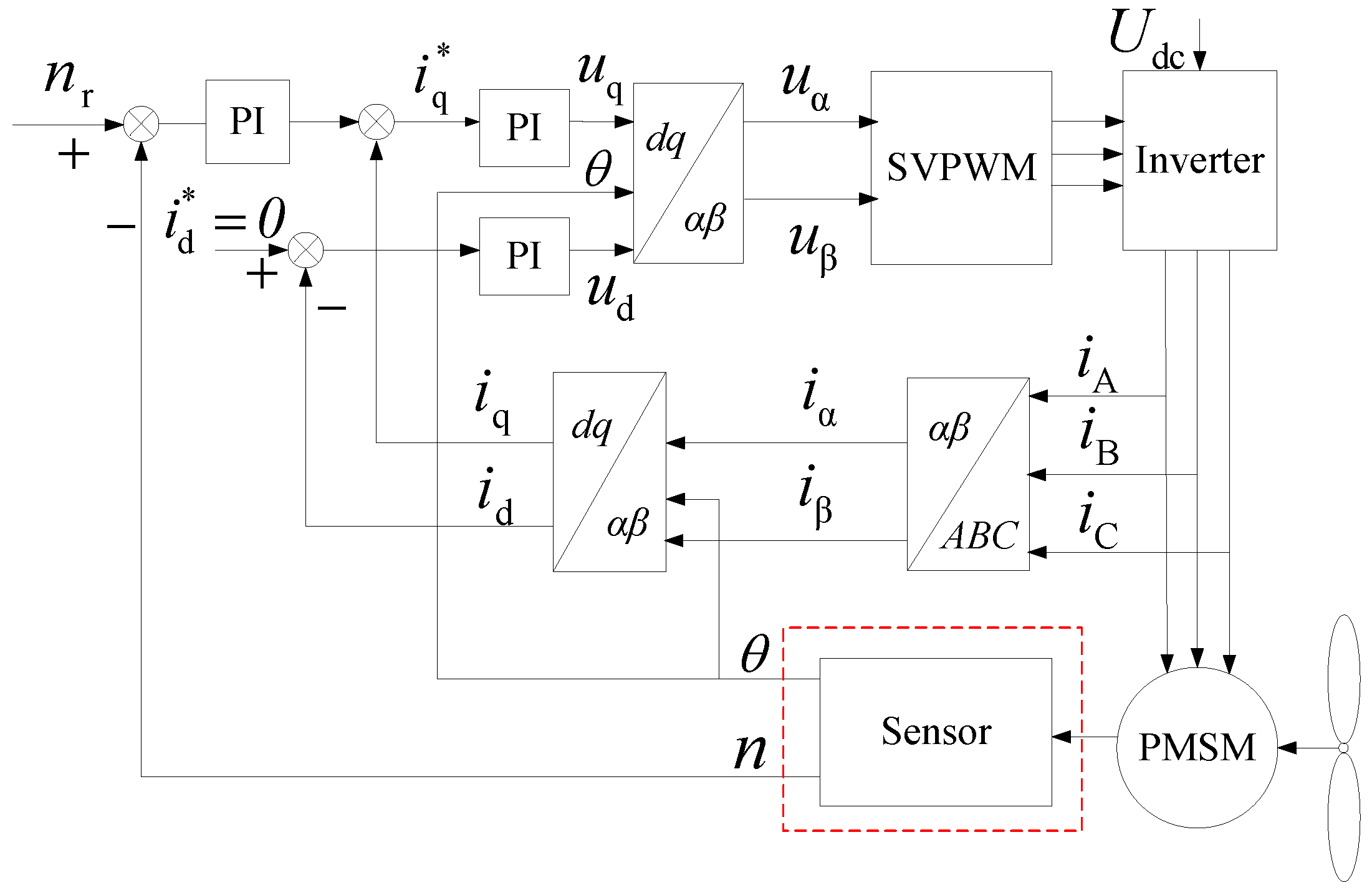
2.1. System Description

The PMSM was used as the prime motor to drive the propeller in the electric propulsion ship system. The propeller propels the ship forward by the ship hull; this principle is shown in Figure 1. It can be seen that the propeller input is motor speed and ship velocity, and the load of propulsion is the ship hull driven by the propeller and the load is impacted by the ocean environment [20].
The thrust P and torque TL of the propeller can be expressed as follows:
{ P = K P ρ n 2 D 4 T L = K M ρ n 2 D 5
where ρ is the sea-water density and ρ = 1025 kg/m3; D is the diameter of the propeller and the unit is meter; n is the speed of the propeller and the unit is r/s; and KP and KM are thrust coefficient and torque coefficient, respectively, and they are both the function of the advance ratio J. After the completion of the ship construction, the relationship between J and KP, KM can be determined by the open water experiment of the ship.
During the operation of the ship, due to the interaction between the hull and water, a wake is generated, which makes the difference between the advance velocity of propeller vp and the actual forward velocity of the ship vs. Therefore, the effective thrust P e and torque TL after considering the increase of the resistance caused by the water absorption of the propeller can be expressed as follows:
{ P e = ( 1 t ) K P ρ n 2 D 4 T L = K M ρ n 2 D 5
where t is the thrust deduction coefficient and t = Δ P P .
When the ship is in motion, the motion equation of its propeller system can be expressed as follows:
( M + Δ M ) d v s d t = P e R
where M is the mass of the ship and the unit is kilogram and Δ M is the mass of the water attached to the ship moving with the ship during movement and usually 5%-15% of the total mass of the hull is taken as the value.
The main factors affecting ship resistance are ship speed, ship type, and environmental conditions (wind, wave, current, etc.) during the operation [21]. When the ship type is determined, the resistance of the ship is only related to the speed of the ship under certain external navigation conditions. The expression is as follows:
R = r v s z
where r is the resistance coefficient and z is the index, and when the ship speed is low, z = 2.

2.2. System Mathematical Model

The PMSM is the main power supply in the electric propulsion ship system, whose performance determines the stability and safety of the whole ship system. We took the three-phase PMSM as propulsion motor, and the mathematical model in the d-q coordinate system is as follows [22].
The equations of stator voltage are the following:
{ u d = R s i d + d ψ d d t ω ψ q u q = R s i q + d ψ q d t + ω ψ d
The equations of stator flux linkage are the following:
{ ψ d = ψ f + L d i d ψ q = L q i q
The equation of electromagnetic torque is the following:
T e = 3 2 n p ( ψ d i q ψ q i d ) = 3 2 n p [ ψ m i q + ( L d L q ) i d i q ]
The dynamic equilibrium equation is the following:
T e T L B ω = J n p d ω d t
where u is voltage; i is current; L is inductance; ψ is flux and the subscripts d and q represent d-axis and q-axis; T e is electromagnetic torque; ψ m is flux produced by the permanent magnet; n p is pole pair number; R s is stator resistance; B is damping coefficient; J is moment of inertia; and ω is mechanical angular velocity.

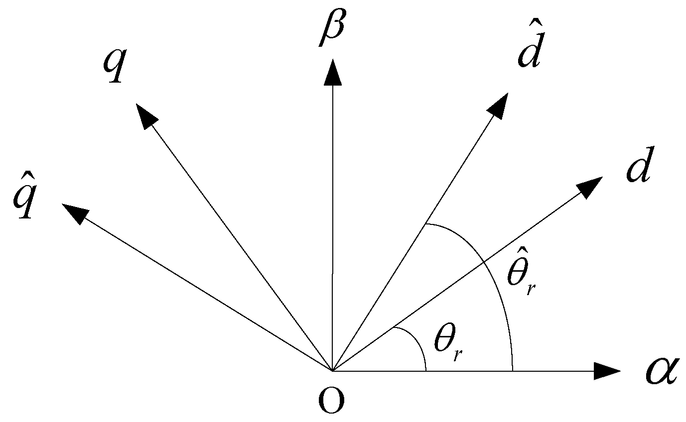
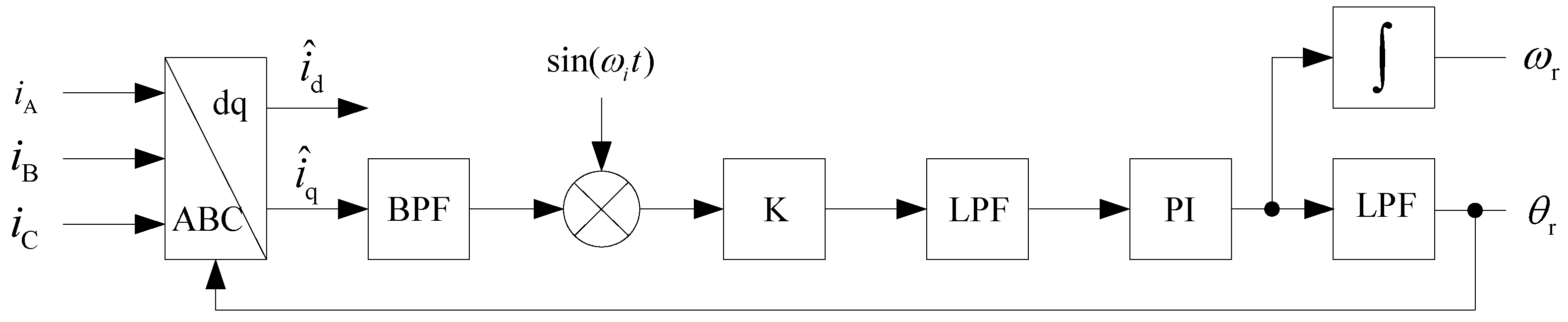
3. Principle of the High-Frequency Voltage Injection Algorithm Based on the SOGI

The PMSM’s vector control principle is shown in Figure 2. In the traditional motor control, the closed-loop speed control can be achieved by mechanical sensors on the motor shaft to obtain the rotor speed and position. On the other hand, in the position sensorless control system, the rotor speed and position are obtained by calculation and the mechanical sensors are cancelled. The HF voltage injection algorithm means injecting the HF voltage into the input voltage port of the motors, where the frequency is 0.5~2k Hz far above the fundamental frequency of motors. Then, the currents are detected and processed to obtain the rotor salient-pole position and speed.
Thus, Equation (5) can be rewritten as follows:
[ u d u q ] = [ R s + L d p ω L q ω L d R s + L q p ] [ i d i q ] + [ 0 ω ψ m ]
where p is the differential operator.
Figure 3 shows the relationships among the different coordinates. It can be seen that α β is a two-phase static coordinate system; d-q is a two-phase rotary coordinate system; d ^ q ^ is the estimated two-phase rotary coordinate system; θ r is the actual rotor position; θ ^ r is the estimated rotor position and the deviation is Δ θ = θ r θ ^ r .
After injecting the HF voltage, which is far above the fundamental frequency, the impact of the permanent magnet flux linkage on HF voltage can be ignored. Thus, Equation (9) can be changed as follows:
[ u d u q ] = [ R s + L d p 0 0 R s + L q p ] [ i d i q ] = [ Z d 0 0 Z q ] [ i d i q ]
From Figure 3, the transformation matrix from the d-q coordinate system to the d ^ q ^ coordinate system can be expressed as follows:
T ( Δ θ ) = [ cos ( Δ θ ) sin ( Δ θ ) sin ( Δ θ ) cos ( Δ θ ) ]
Thus, the estimated voltages are as follows:
[ u ^ d u ^ q ] = T ( Δ θ ) [ u d u q ] = T ( Δ θ ) [ Z d 0 0 Z q ] [ i d i q ] = T ( Δ θ ) [ Z d 0 0 Z q ] T 1 ( Δ θ ) [ i ^ d i ^ q ]
Equation (12) can be transformed and the estimated currents can be obtained as follows:
[ i ^ d i ^ q ] = T ( Δ θ ) [ 1 Z d 0 0 1 Z q ] T 1 ( Δ θ ) [ u ^ d u ^ q ] = 2 Z 2 Δ Z 2 [ Z Δ Z cos ( 2 θ ) Δ Z sin ( 2 θ ) Δ Z sin ( 2 θ ) Z + Δ Z cos ( 2 θ ) ] [ u ^ d u ^ q ]
The injected HF voltage is as follows:
[ u ^ d u ^ q ] = U m [ cos ( ω i   t ) 0 ]
The estimated currents in d ^ q ^ coordinate are as follows:
{ i ^ d = 2 ( Z Δ Z cos ( 2 Δ θ ) ) Z 2 Δ Z 2 U m cos ( ω i t ) i ^ q = 2 Δ Z sin ( 2 Δ θ ) ) Z 2 Δ Z 2 U m cos ( ω i t )
where Z = Z d + Z q , Δ Z = Z d Z q .
For the HF inductance, the resistance is small enough and can be cancelled. Thus, Equation (15) can be simplified as follows:
{ i ^ d = 2 ( ω i L ω i Δ L cos ( 2 Δ θ ) ) ( ω i L ) 2 ( ω i Δ L ) 2 u i sin ( ω i t ) = u i sin ( ω i t ) ω i ( L 2 Δ L 2 ) ( L Δ L cos ( 2 Δ θ ) ) i ^ q = 2 ω i Δ L sin ( 2 Δ θ ) ) ( ω i L ) 2 ( ω i Δ L ) 2 u i sin ( ω i t ) = u i sin ( ω i t ) ω i ( L 2 Δ L 2 ) Δ L sin ( 2 Δ θ ) )
when Δ θ = 0 , there is a deviation value in i ^ d . It can be seen from the property of the sine function, i ^ q Δ θ , and if Δ θ 0 , i ^ q 0 . Therefore, the estimated rotor position can be converged to the real value by processing the q ^ -axis currents [23]. Then, the d-axis and q-axis estimated currents can be transformed by three-phase currents. The HF components of the q-axis estimated currents are obtained by bandwidth filters and are then multiplied by the modulating signal sin ( ω i   t ) . The input of the regulator can be obtained by low-pass filter, which is shown in Figure 4. When Δ θ is small enough, sin ( 2 Δ θ ) = 2 Δ θ , and
F ^ ( Δ θ ) = u ih Δ L ω i ( L 2 Δ L 2 ) sin ( 2 Δ θ ) u ih Δ L ω i ( L 2 Δ L 2 ) 2 Δ θ
The basic structure of the SOGI is shown in Figure 5. It can be seen that the SOGI is formed by two second-order generalized integrators, which can have output signals that are orthogonal to each other and do not delay [24]. Equation (18) shows the transfer functions of the three system outputs, y1, y2, and y3. Among them, the role of y1 is to eliminate the harmonics of frequency ω, the role of y2 is to extract the harmonics of frequency ω, and the frequency of y3 is ω and it is orthogonal to y2 [25].
{ y 1 x = s 2 + ω 2 s 2 + k ω s + ω 2 y 2 x = k ω s s 2 + k ω s + ω 2 y 3 x = k ω 2 s 2 + k ω s + ω 2
The improved position observer structure combining the SOGI and HF injection is shown in Figure 6. The rotor position observer includes two components, I and II. The input of part I is the estimated q-axis voltage. The output y2 is the HF voltage component in the estimated q-axis, which is used to extract the HF component in the input q-axis voltage. ωe1 is the frequency of the HF signal to be extracted. When the HF component u ^ qh is multiplied by the HF cosine modulation signal cos ( ω h   t ) of the same phase, it enters part II. The input of the modulated value u is the value after modulation u ^ qh and cos ( ω h   t ) , and the output y1 is the rotor position error information fcθ), which is used to suppress the harmonic of a specific frequency, so as to extract the rotor position information accurately. In the control, the filtering effect and response speed should be weighed to determine the parameter values.

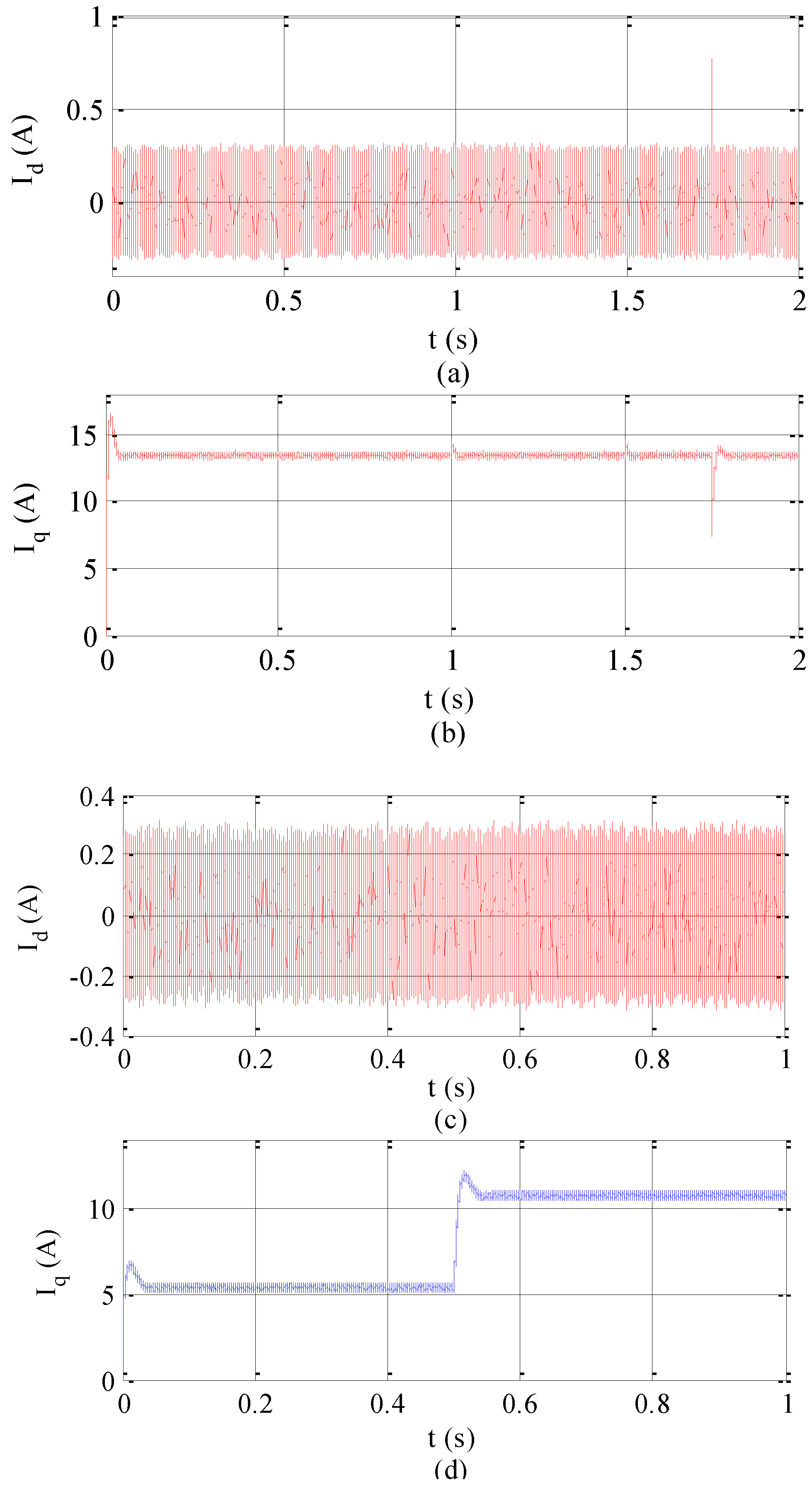
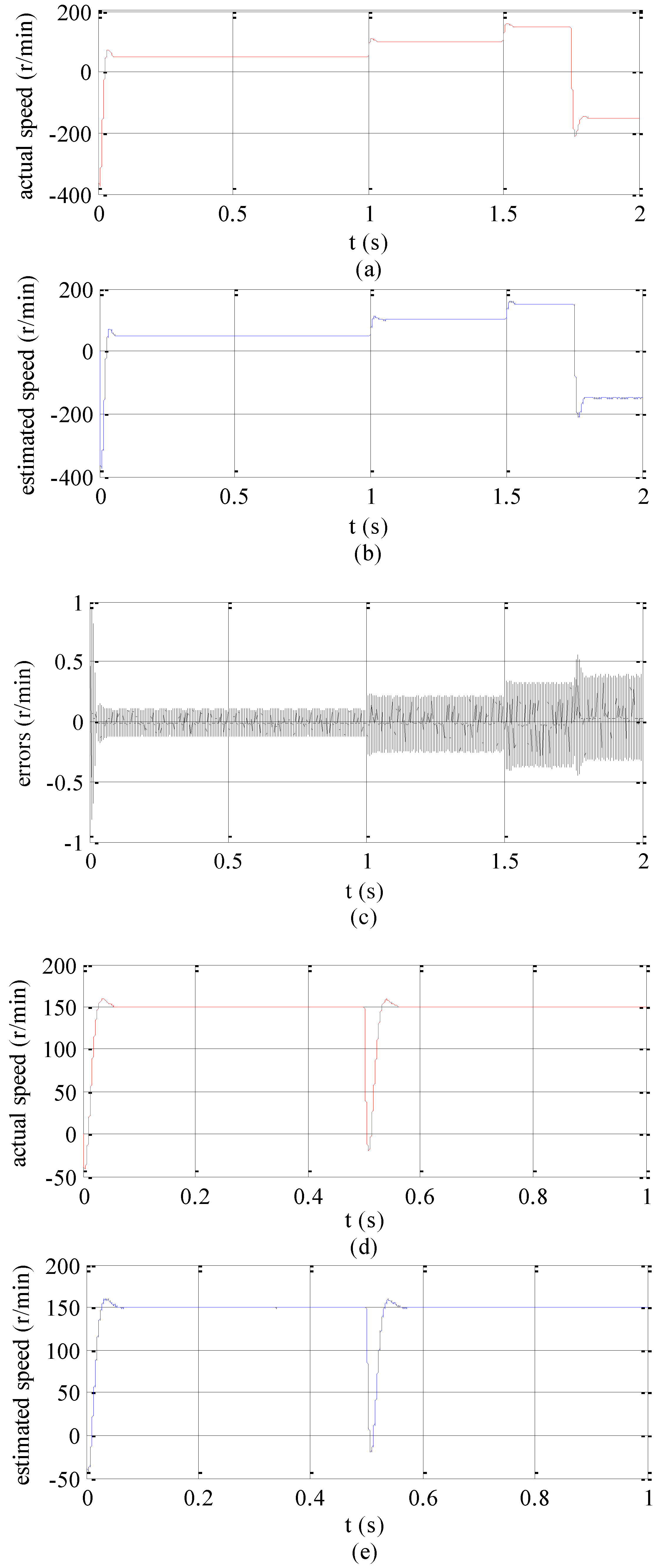
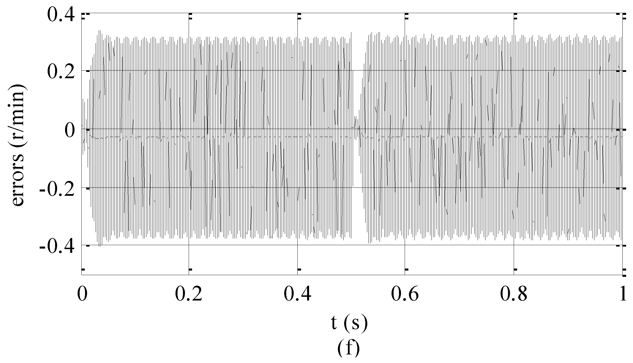
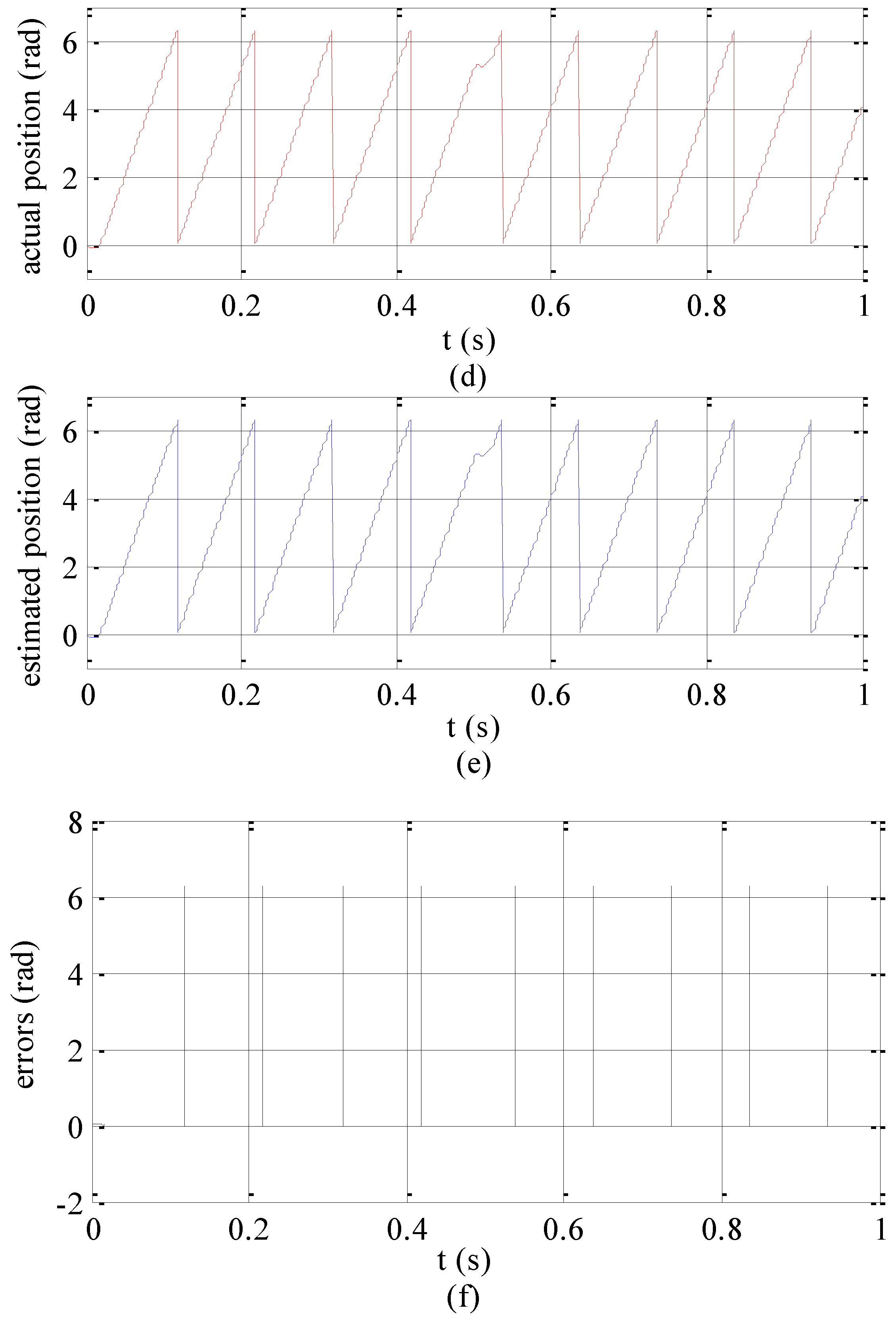
4. Simulation Analysis

The theoretical speed range that the HF injection algorithm with the SOGI can estimate accurately is 10 r/min to 300 r/min. Therefore, we chose different speeds to verify in the simulation. The rotor position estimation model of the PMSM and the whole electric propulsion ship system were built in MATLAB/Simulink according to the vector control principle and the HF voltage injection algorithm with the SOGI. The required motor simulation parameters are shown in Table 1.
The motor starts with TN = 2 Nm and the initial speed n = 50 r/min. At t = 1 s, the speed jumps to 100 r/min; at t = 1.5 s, the speed jumps to 150 r/min; and at t = 1.75 s, the speed reverses to −150 r/min. At n = 150 r/min, the given load jumps to 4 Nm at t = 0.5 s in the second simulation. The simulation waveforms are shown in Figure 7, Figure 8 and Figure 9.
Figure 7 gives the waveforms of the d-axis and q-axis currents. The q-axis currents are related to the torque and estimated rotor position and they fluctuate with the changes of speed from Figure 7b. It can be seen in Figure 7d that the changes of the q-axis currents agree with the changes of the torque, which conforms to theoretical analysis. In addition, the current on the d-axis is near zero from Figure 7a,c.
Figure 8 displays the waveforms of rotor speed. It can be seen from Figure 8a,b that actual speed and estimated speed are very close during the steady operation. There are large deviations only at the start, at the moment of load change and speed change. As seen in Figure 8c, the deviations are close to zero. Furthermore, at n = 50 r/min, the ripples are at 0.4%, at n = 100 r/min, the ripples are at 0.5%, at n = 150 r/min, the ripples are at 0.53%, and at n = -150r/min, the ripples are at 0.67%. In the second simulation with torque changes, the speed can also be estimated accurately from Figure 8d–f.
Figure 9 are the waveforms of rotor position. It can be seen that actual position and estimated position are very close and the estimated position slightly lags behind the actual position from Figure 9a,b,d,e, and there is a large deviation only when the rotor runs a full circle, which is shown in Figure 9c,f. In the other operation stages, the errors are in the range of 0.05 rad to 0.2 rad from Figure 9c,f.
A comprehensive simulation model of the electric propulsion ship system is constructed by taking the output torque of the propeller model as the load torque of the PMSM and the motor speed as the input of the propeller model. When the propulsion motor is started, the given speed is 100 r/min. At t = 3 s, the speed jumps to 170 r/min. The estimated rotor position and speed are taken as feedback signals during operation and the waveforms of the propulsion motor speed and torque are shown in Figure 10. At the beginning, the motor is in an accelerated state, and the output torque of the propeller model, namely the load torque of the propulsion motor, increases with the increase of the rotating speed. After about 0.5 s, the speed stabilizes at 100 r/min. At that time, the load torque of the motor starts to decrease and gradually stabilizes. After 3 s, with the re-acceleration of the motor, the load torque also begins to increase. Until the propulsion motor runs stably at 170 r/min, the load torque began to decrease and finally stabilizes. The results show that the HF injection position estimation strategy can be applied to the whole ship system.
From the above simulation waveforms, it can be seen that the HF injection algorithm based on the SOGI can estimate the rotor speed accurately within acceptable deviations. Furthermore, the whole electric propulsion ship system can also operate normally with the sensorless control strategy.

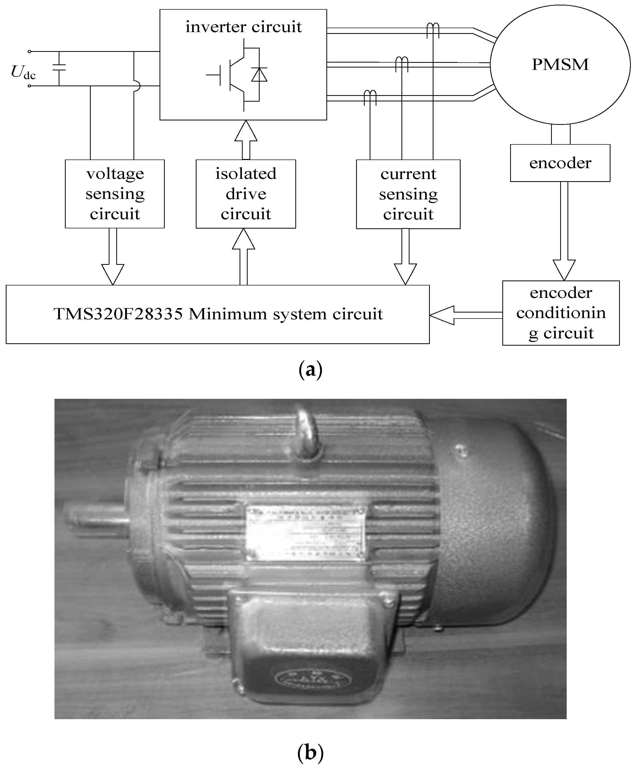
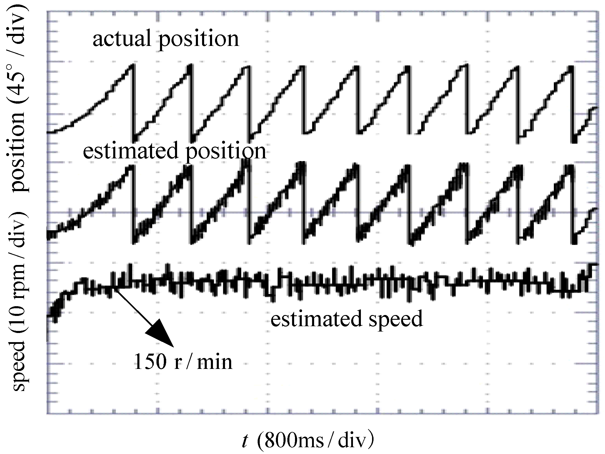
5. Experimental Analysis

To further verify the accuracy of the proposed HF injection algorithm based on the SOGI, the diagram of the system hardware structure and the experimental setup of the electric propulsion ship in the laboratory are shown in Figure 11, in which the TMS320F28335 DSP was adopted as the digital controller. The experimental motor parameters are the same as the simulation parameters. The speed is obtained by speed sensors; the currents are obtained by the current probe and displayed on the oscilloscope; the torque is calculated according to the measured currents.
The experimental waveforms of rotor position and speed are shown in Figure 12. The actual position is measured by mechanical sensor and the estimated rotor position is obtained using the calculation from the HF injection algorithm with the SOGI. It can be seen that the estimated values fluctuate within a certain range around the actual value.
To sum up, the HF injection algorithm based on the SOGI can estimate the rotor position and speed accurately at low speed in the experimental PMSM and it is applicable in the PMSM system.

6. Conclusions

It is inevitable that the electric propulsion ship will replace the traditional diesel engine propulsion ship, and it is significant to study the control method of the propulsion PMSM in the electric propulsion ship system. The HF injection position estimation algorithm based on the SOGI is proposed on the basis of analyzing the structure of the electric propulsion ship system and the vector control of the PMSM. The algorithm can be used to estimate the rotor position and speed at low speed in the electric propulsion ship system within acceptable deviations. In fact, the position sensorless control technology can represent the redundancy of the control system with sensors. Subsequently, when there is a fault in the mechanical sensors, the control system can switch to the sensorless operating control mode, which can further improve the reliability of the electric propulsion ship system.

Funding

This research received no external funding.

Conflicts of Interest

The authors declare no conflict of interest.

References

  1. Ren, J.; Liu, Y.; Wang, N.; Liu, S. Sensorless control of ship propulsion interior permanent magnet synchronous motor based on a new sliding mode observer. ISA Trans. 2015, 54, 15–26. [Google Scholar] [CrossRef] [PubMed]
  2. Bai, H.; Zhu, J.; Qin, J. Performance study of three-phase fault-tolerant permanent magnet motor drive for marine propulsion system based on structure design. J. Ship Res. 2017, 61, 23–34. [Google Scholar] [CrossRef]
  3. He, Z.; Jia, Z.; Zhu, L.; Zhang, F. Performance analysis of sliding mode position observer for marine SPMSM sensorless control. In Proceedings of the PEAC, Shenzhen, China, 4–7 November 2018. [Google Scholar]
  4. Li, H.; Wang, Z. Sensorless control for PMSM drives using the cubature Kalman filter based speed and flux observer. In Proceedings of the ESARS-ITEC, Nottingham, UK, 7–9 November 2018. [Google Scholar]
  5. Hoque, M.A.; Rahman, M. Speed and position sensorless permanent magnet synchronous motor drives. In Proceedings of the CCECE. 1994, pp. 689–692. Available online: https://research.library.mun.ca/5398/ (accessed on 2 February 2020).
  6. Lu, K.; Lei, X.; Blaabjerg, F. Artificial inductance concept to compensate nonlinear inductance effects in the back EMF-based sensorless control method for PMSM. IEEE Trans. Energy Convers. 2013, 28, 593–600. [Google Scholar] [CrossRef]
  7. Song, X.; Fang, J.; Han, B.; Zheng, S. Adaptive compensation method for high-speed surface PMSM sensorless drives of EMF-based position estimation error. IEEE Trans. Power Electron. 2016, 31, 1438–1449. [Google Scholar] [CrossRef]
  8. Bao, D.; Wang, Y.; Pan, X.; Wang, X.; Li, K. Improved sensorless control method combining SMO and MRAS for surface PMSM drives. In Proceedings of the IAS, Cincinnati, OH, USA, 1–5 October 2017; pp. 1–5. [Google Scholar]
  9. Liang, D.; Li, J.; Qu, R. Sensorless control of permanent magnet synchronous machine based on second-order sliding-mode observer with online resistance estimation. IEEE Trans. Ind. Appl. 2017, 53, 3672–3682. [Google Scholar] [CrossRef]
  10. Xu, D.; Wang, B.; Zhang, G.; Wang, G.; Yu, Y. A review of sensorless control methods for AC motor drives. CES Trans. Electr. Mach. Syst. 2018, 2, 104–115. [Google Scholar]
  11. Wang, G.; Kuang, J.; Zhao, N.; Zhang, G.; Xu, D. Rotor position estimation of PMSM in low-speed region and standstill using zero-voltage vector injection. IEEE Trans. Power Electr. 2018, 33, 7948–7958. [Google Scholar] [CrossRef]
  12. Jang, J.H.; Sul, S.K.; Ha, J.I.; Ide, K.; Sawamura, M. Sensorless drive of surface-mounted permanent-magnet motor by high-frequency signal injection based on magnetic saliency. IEEE Trans. Ind. Appl. 2003, 39, 1031–1039. [Google Scholar] [CrossRef]
  13. Wang, S.; Yang, K.; Chen, K. An improved position-sensorless control method at low speed for PMSM based on high-frequency signal injection into a rotating reference frame. IEEE Access 2019, 7, 86510–86521. [Google Scholar] [CrossRef]
  14. Moghadam, M.; Tahami, F. Sensorless control of PMSMs with tolerance for delays and stator resistance uncertainties. IEEE Trans. Power Electr. 2013, 28, 1391–1399. [Google Scholar] [CrossRef]
  15. Reigosa, D.; Fernandez, D.; Yoshida, H.; Kato, T.; Briz, F. Permanent-magnet temperature estimation in PMSMs using pulsating high-frequency current injection. IEEE Trans. Ind. Appl. 2015, 51, 3159–3168. [Google Scholar] [CrossRef]
  16. Busada, C.; Jorge, S.; Leon, A.; Solsona, J. Current controller based on reduced order generalized integrators for distributed generation systems. IEEE Trans. Ind. Electr. 2012, 59, 2898–2909. [Google Scholar] [CrossRef]
  17. Liu, B.; Zhou, B.; Ni, T.H. Enhanced position observer with a selective harmonic error eliminator and an error feed-forward compensator for sensor-less surface-mounted permanent magnet synchronous motor drives. In Proceedings of the IFEEC-ECCE Asia, Kaohsiung, Taiwan, 3–7 June 2017; pp. 1210–1214. [Google Scholar]
  18. Zhang, G.; Wang, G.; Xu, D.; Fu, Y.; Ni, R. Adaptive notch filter based rotor position estimation for interior permanent magnet synchronous motors. Proc. CSEE 2016, 36, 2521–2527. (In Chinese) [Google Scholar]
  19. Yao, W.; Liu, Y.; Yin, Z.; Zeng, D.; Li, H. Speed sensorless vector control of marine podded propulsion motor based on strong track filter. In Proceedings of the CCDC, Qingdao, China, 23–25 May 2015; pp. 1882–1887. [Google Scholar]
  20. Sulligoi, G.; Vicenzutti, A.; Menis, R. All-electric ship design: From electrical propulsion to integrated electrical and electronic power systems. IEEE Trans. Power. Electr. 2016, 2, 507–521. [Google Scholar] [CrossRef]
  21. Ahmadi, R.; Behjati, H.; Ferdowsi, M. Dynamic modeling and stability analysis of an experimental test bench for electric-ship propulsion. In Proceedings of the 2013 IEEE Electric Ship Technologies Symposium, Arlington, VA, USA, 22–24 April 2013; pp. 110–115. [Google Scholar]
  22. Wang, G.; Ding, L.; Li, Z.; Xu, J.; Zhang, G.; Zhan, H.; Ni, R.; Xu, D. Enhanced position observer using second-order generalized integrator for sensorless interior permanent magnet synchronous motor drives. IEEE Trans. Energy Convers. 2014, 29, 486–495. [Google Scholar]
  23. Szalai, T.; Berger, G.; Petzoldt, J. Stabilizing sensorless control down to zero speed by using the high-frequency current amplitude. IEEE Trans. Power Electr. 2014, 29, 3646–3656. [Google Scholar] [CrossRef]
  24. Liu, B.; Zhou, B.; Ni, T. Principle and Stability Analysis of an Improved Self-Sensing Control Strategy for Surface-Mounted PMSM Drives Using Second-Order Generalized Integrators. IEEE Trans. Energy Convers. 2018, 33, 126–136. [Google Scholar] [CrossRef]
  25. Liu, B.; Zhou, B.; Wei, J.; Wang, L.; Ni, T. A novel method for polarity detection of nonsalient PMSMs in initial position estimation. In Proceedings of the APEC, Long Beach, CA, USA, 20–24 March 2016; pp. 2754–2758. [Google Scholar]
Figure 1. Relationship of ship, motor, and propeller.
Electronics 09 00276 g001
Figure 2. Vector control system of a permanent magnet synchronous motor (PMSM) applied in ships.
Electronics 09 00276 g002
Figure 3. Relationship between the three coordinate systems.
Electronics 09 00276 g003
Figure 4. Estimation process of rotor position.
Electronics 09 00276 g004
Figure 5. Basic structure of the second-order generalized integrator (SOGI).
Electronics 09 00276 g005
Figure 6. Principle of the improved position observer structure.
Electronics 09 00276 g006
Figure 7. Waveforms of currents in d-axis and q-axis: (a) d-axis current with speed changes; (b) q-axis current with speed changes; (c) d-axis current with torque changes; (d) q-axis current with torque changes.
Electronics 09 00276 g007
Figure 8. Waveforms of rotor speed: (a) actual rotor speed with speed changes; (b) estimated rotor speed with speed changes; (c) errors between actual rotor speed and estimated rotor speed with speed changes; (d) actual rotor speed with torque changes; (e) estimated rotor speed with torque changes; (f) errors between actual rotor speed and estimated rotor speed with torque changes.
Electronics 09 00276 g008aElectronics 09 00276 g008b
Figure 9. Waveforms of rotor position: (a) actual rotor position with speed changes; (b) estimated rotor position with speed changes; (c) errors between actual rotor position and estimated rotor position with speed changes; (d) actual rotor position with torque changes; (e) estimated rotor position with torque changes; (f) errors between actual rotor position and estimated rotor position with torque changes.
Electronics 09 00276 g009aElectronics 09 00276 g009b
Figure 10. Waveforms of propulsion motor speed and torque: (a) propulsion motor speed; (b) propulsion motor torque.
Electronics 09 00276 g010
Figure 11. Experimental setup of the PMSM: (a) system hardware structure; (b) experimental PMSM; (c) control circuit.
Electronics 09 00276 g011aElectronics 09 00276 g011b
Figure 12. Experimental results of rotor position and speed.
Electronics 09 00276 g012
Table 1. Parameters of the PMSM.
SymbolQuantityValues
npnumber of pole pairs2
Rstator resistance1.51 Ω
Ldwinding inductance0.0048 mH
Lqwinding inductance0.0134 mH
Jrotational inertia0.000244 kg.m2
Bdamping coefficient0.0002517
Ψfrotor flux0.1073 Wb
Udcdirect voltage380 V
Prated power1 kW

