A Fault Diagnosis Strategy Based on Multilevel Classification for a Cascaded Photovoltaic Grid-Connected Inverter

Abstract

In this paper, an effective strategy is presented to realize IGBT open-circuit fault diagnosis for closed-loop cascaded photovoltaic (PV) grid-connected inverters. The approach is based on the analysis of the inverter output voltage time waveforms in healthy and faulty conditions. It is mainly composed of two parts. The first part is to select the similar faults based on Euclidean distance and set the specific labels. The second part is the classification based on Principal Component Analysis and Support Vector Machine. The classification is done in two steps. In the first, similar faults are grouped to do the preliminary diagnosis of all fault types. In the second step the similar faults are discriminated. Compared with existing fault diagnosis strategies for several fundamental periods and under different external environments, the proposed strategy has better robustness and higher fault diagnosis accuracy. The effectiveness of the proposed fault diagnosis strategy is assessed through simulation results.

1. Introduction

Among the renewable energies promoted worldwide due to the environmental issues, photovoltaic (PV) energy systems are one of the most promising due to its lower environmental impact and abundance [1]. However, the connection of PV plant to the power utility grid was limited because of voltage mismatch and grid code requirements that could not be met. Thanks to the development of power converters and their control, PV plants can be connected without degrading the energy conversion efficiency thanks to the low switching frequency of cascaded multilevel inverters [2]. One key aspect in power electronic system is reliability [3], for those applications that consider availability as a critical parameter, it is important that the application continues to operate even under faulty conditions. For PV grid-connected system, the performance of the inverter is one of the key factors that determine whether the system can continue to operate. Open-circuit and short-circuit faults are the most common faults affecting inverters. Since most modern gate-drivers are equipped with short-circuit protection unit, open-circuit fault attracts more attention [4]. Figure 1a shows the application of PV grid-connected system and Figure 1b shows the consequence of photovoltaic inverter fires. Once the fault occurs, the output voltage is distorted and the produced power is degraded. If it cannot be diagnosed and repaired in time, a derivative fault will occur, which may seriously lead to system crash.

The literature on fault diagnosis methods is abundant [6] but for each system, an appropriate strategy is required. For PV grid-connected systems there are many studies on the closed-loop control. However, for the purpose of health monitoring, most of the studies are conducted considering that the system is in open loop, which is not the usual case [7,8,9]. Moreover, fault diagnosis of PV systems cannot ignore the variability of the irradiance and the temperature induced by the environmental conditions. Indeed, this variability influences the inverter output voltage. Therefore, the results presented in [10,11,12,13] which only consider one environmental condition for PV inverter fault diagnosis, are limited in scope. Fault diagnosis methods can be decomposed in four steps: modelling, pre-processing, feature extraction and feature analysis for fault detection, fault classification and fault estimation [14]. In the following, only fault detection and fault classification will be discussed. Fault features can be extracted from different signals obtained from raw measurements in the time domain or transformed into another domain that can be time-frequency, time-scale or frequency. Different techniques can be used to extract and analyze the fault features ranging, e.g., from signal or information processing tools or machine-learning tools.

Here are some examples of signal-processing-based methods. Authors in [15] have proposed a relative weighting operator of principal component analysis (PCA) to extract the fault information of a cascaded inverter. In Reference [16], a multilevel signal decomposition and coefficients reconstruction method is used to generate the multiscale features for fault feature extraction. In [17], authors adopted a second low frequency processing (SLFP) method to obtain the small low-frequency data from the feedback controller. Authors in [18] have used the average bridge arm pole-to-pole (PTP) voltage and error-adaptive thresholds of the inverter to extract the fault information. In [19], an adaptive confidence limit (ACL) fault detection method is proposed to process the changing signals. The main drawbacks of these methods are their sensitivity to frequency resolution and environmental nuisances.

Machine-learning methods are becoming more and more attractive in engineering applications. Authors in [20] have designed a new generator and discriminator of Generative Adversarial Network (GAN) to extract more fault features from Auto Encoder (AE). In Reference [21], authors have proposed a multiclass Relevance Vector Machine (mRVM) to achieve higher model sparsity and shorter diagnosis time. In Reference [22], intuitionistic fuzzy logic is integrated to original spiking neural P systems for dealing with the uncertain knowledge of the power system. Authors in [23] have adopted Genetic Algorithm (GA), Particle Swarm Optimization (PSO) and Cuckoo Search Algorithm (CSA) methods to optimize the neural network in order to have the lowest mean square error.

On one hand, machine learning methods are highly adaptable and do not rely on accurate mathematical models [24]. On the other hand, they need a large amount of data (representing several operating conditions) for training the network, a significant experience to set a large number of parameters, and the effect of each algorithm is very different for different types of input. The computational cost may also constitute an obstacle to its implementation in real engineering applications.

From the above discussion, we can conclude that time-domain analysis using signal and information processing tools may be more suitable for developing an inverter fault diagnosis method for PV grid-connected inverter system. In addition, the method should be able to cope with the closed-loop behavior and be robust to the variations of the environmental conditions (irradiance and temperature). The fault diagnosis strategy proposed in this paper is based on principle component analysis (PCA) and support vector machine (SVM). It consists of three parts. The first part is devoted to group the similar faults based on Euclidean distance and set the specific labels. The second part is the first classification level based on PCA-SVM. PCA is known as one of the most common multivariate statistical process control (MSPC) methods for dimensionality reduction while retaining the meaningful information [25]. After the feature extraction, the fault classification is performed with SVM, a classical algorithm for pattern classification. It has better generalization capability than artificial neural networks (ANN), and guarantees that local and global optimal solutions are identical [26]. The third part is the second classification level. PCA and two-class SVM are used to discriminate the similar faults. The performances of the overall method are evaluated for different environmental conditions.

The fault diagnosis process consists of four steps: modeling, pre-processing, features extraction and features analysis.

The first step is devoted to knowledge building. It can be done through physics-based equations, language-based models or data-driven. In the second step, the input data is pre-processed. The data can be filtered to reduce the nuisances or transformed from time domain to frequency domain or time-frequency domain or projected into another reference frame. The objective of this step is to prepare the information from which the best features will be extracted in the third step. In this third step the fault signatures can be extracted with different techniques ranging from signal processing, information processing and control theory for example. In the last step, the features are analyzed to decide whether a fault has occurred, to classify the different fault types, isolate the faults and eventually estimate the fault severities.

In our study we take benefit of the measured output voltage historical data to model our system. Depending on the applications one can use different signals like vibration, acoustic, phase current or electromagnetic field. Vibration and acoustic signals are most usually used to diagnose mechanical faults. In energy conversion systems the phase currents are very popular. However, in our application the current depends on the load requirement, which varies continuously during daytime. There are many papers [27,28,29] that have already proposed multi-level inverter fault diagnosis using voltage spectral analysis. However, in order to avoid any additional transformation such as Fast Fourier Transform (FFT) or Wavelet Transform, we have decided to exploit the voltage characteristics in the time domain.

Moreover, in multi-level converters [30], the shape of the output voltage depends on the states of the power switches. Therefore, any fault affecting the power converter will directly modify the shape of the output voltage.

This paper is outlined as follows. In Section 2, the open-circuit fault features of a cascaded five-level inverter in closed-loop PV grid-connected system are analyzed under different external environments. In Section 3, the proposed fault diagnosis strategy is presented. In Section 4, the effectiveness of the proposed strategy is evaluated for several operating time durations and under different environmental conditions through numerical simulations. Finally, the conclusion is provided in Section 5.

2. Problem Description

The cascaded five-level inverter for a single-phase PV grid-connected system is shown in Figure 2 [31], which is mainly composed of PV sources, two H-bridge inverters connected in series, inductive filter and the public grid. PV voltages, PV currents, grid current and grid voltage are required to generate control signals for the closed-loop control strategies of Maximum Power Point Tracking (MPPT), voltage and current control loops and power balance control.

In this PV system, the two H-bridges are composed of eight IGBTs. Since the most common faults in the industry are single IGBT open-circuit faults [32]; in this paper, the healthy state of nine conditions will be analyzed, alongside eight single IGBT open-circuit faults.

2.1. Similar Faults

Figure 3 shows the healthy state and eight IGBTs ($S_1~S_8$) open-circuit output voltage waveforms. At fault occurrence (t = 0.2 s) the output voltage waveform is distorted and after a transient it gradually stabilizes due to the closed-loop adjustment. When analyzing these eight IGBTs open-circuit waveforms, we have found a fault diagnosis accuracy of 80% in [33], 85% in [34] and 90% in [35]. We can also deduce from Figure 3 that there are two groups of similar output voltage waveforms as shown in

Table 1. Similar faults.

Group Number	Fault Type
1	S2 open-circuit and S3 open-circuit
2	S5 open-circuit and S8 open-circuit

. The high similarity makes them difficult to distinguish. The $S_2$ and $S_3$ open-circuit faults are in group 1 while $S_5$ and $S_8$ open-circuit faults are in group 2. In the following, due to page limitation, we will focus only on feature analysis of data for the similar faults. Taking group 1 as an example, the inverter output voltage waveforms over several periods and under different environmental conditions will be analyzed in detail.

2.2. The Impact of Different Fundamental Periods and Different Environmental Conditions

In order to illustrate the effect of different fundamental periods and different environmental conditions on the fault waveforms, two conditions are chosen for $S_2$ and $S_3$ open-circuit faults for 10 periods, as shown in Figure 4 and Figure 5. The environmental condition 1 is 9:00 a.m. on February 18th: the solar irradiation intensity is 224 W/m², temperature is 4.5 °C; the environmental condition 2 is 13:00 p.m. on August 18th: the solar irradiation intensity is 698 W/m², temperature is 28.9 °C (the data is acquired from Harnhill and Diddington in the U.K [36]).

Figure 4 shows the inverter output voltage waveform over 10 periods under condition 1. At fault occurrence at 0.2 s, the output voltage waveforms fluctuate in a period of time due to the self-regulating effect of the closed-loop system. We take the moment when the fault occurs as the beginning of the first period $T_1$; $T_n(n=1,2,\dots ,10)$ represents a sequence of fundamental periods—each fundamental period is equal to 0.02 s.

Figure 5 shows the inverter output voltage waveforms over 10 periods when S₂ and S₃ open-circuit faults occur at 0.2 s under condition 2. We can notice from Figure 4 and Figure 5 that despite the same fault there are some differences due to the different environmental conditions. To show the differences more clearly, Euclidean distance is calculated between S₂ and S₃ open-circuit faults in each period under each environmental condition (after standardization). The results are plotted in Figure 6. The first two periods correspond to the healthy state (denoted as $H$), so the Euclidean distances are close to zero. At fault occurrence, the Euclidean distances clearly change. The distances increase during the periods $T_1$ and $T_2$, before decreasing gradually due to the control loops actions. We can also notice slight differences for the two environmental conditions.

The former analysis has pointed out that the output voltage waveform is sensitive to the inverter IGBT open-circuit fault. However, the results also show that the waveform is affected by the dynamics of closed-loop action and the variations of the environmental conditions (the irradiance and the temperature). The results also show that some faults have similar signatures. All these issues should be addressed using the fault diagnosis method detailed in the following section.

3. Fault Diagnosis Strategy Based on Multilevel Classification

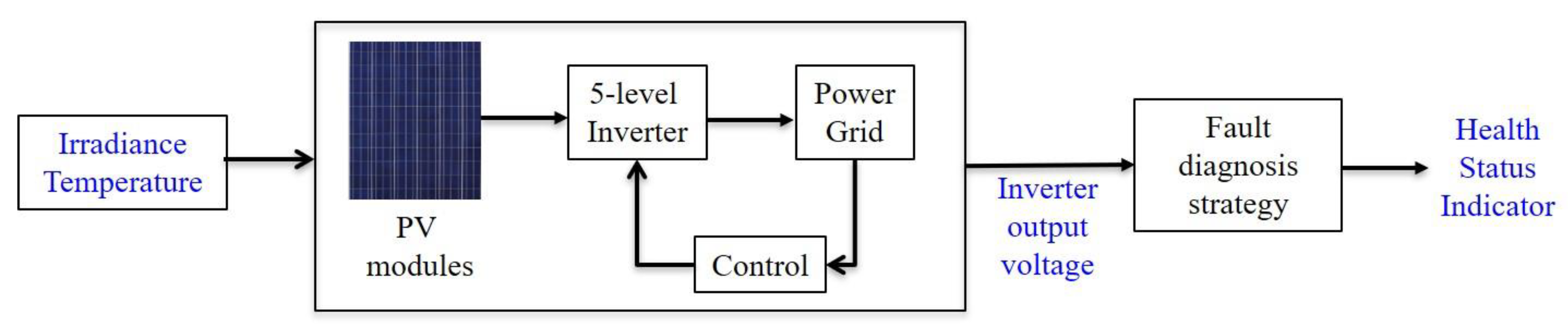
As shown in Figure 7, a block diagram of grid-connected PV plant fault diagnosis is illustrated. The DC supply of 5-level inverter is from PV modules, which is influenced by solar irradiance and temperature. The output of 5-level inverter is connected to the grid by control strategies. The output voltage of the inverter is collected as the fault diagnosis signals and through the proposed fault diagnosis strategy, the health status of the 5-level inverter is monitored. In this section, the fault diagnosis strategy is focused on described in detail, which is contained three parts: data standardization and faults labeling, the first classification level for all fault types and the second classification level for the faults with similar signatures.

3.1. Data Standardization and Faults Labeling

In order to reduce the influence of the dimension and the wide range of variation of the inverter output voltage on the fault diagnosis, the first step is to standardize the input signals using the Z-score method. Let X_[N×m] be the original data matrix, where m is the number of variables and $N$ is the number of samples. The matrix is given by:

X_[N×m] = [x₁, x₂, ⋯, x_j, ⋯, x_m],

(1)

where ${\mathit{x}}_j(j=1,2,\cdots ,m)$ is the $jth$ observation. The Z-score formula is expressed as:

$$z_{ij}=\frac{x_{ij}-\overline{x_j}}{{\sigma }_j},\mathrm{for}i=1,2,\cdots N,j=1,2,\cdots m$$

(2)

where $x_{ij}$ is the $ith$ sample of the $jth$ observation, $\overline{x_j}$ and ${\sigma }_j$ are respectively the mean value and the standard deviation of the $jth$ observation.

Hence, the standardized matrix after Z-score is given by:

$${\mathit{Z}}_{[N\times m]}=[{\mathit{z}}_1,{\mathit{z}}_2,\cdots ,{\mathit{z}}_j,\cdots ,{\mathit{z}}_m],$$

(3)

The second step is to add category labels for the different fault types. In the previous section we have shown that some faults have similar signature. Therefore, in our approach, we will develop a multi-level fault classification. In the first level, faults with similar signatures are merged in the same group and distinguished from other faults. In the second level, they will be discriminated. In this paper we introduce Euclidean distance to group similar faults. Assume that there are $h$ kinds of faults, denoted as ${\mathit{F}}_1,{\mathit{F}}_2,\cdots ,{\mathit{F}}_h$, each kind of fault containing $p$ features. Considering two faults ${\mathit{F}}_v$ and ${\mathit{F}}_w$ their Euclidean distance $dist({\mathit{F}}_v,{\mathit{F}}_w)$ is computed and compared to a threshold. If equation (4) is verified, the two faults ${\mathit{F}}_v$ and ${\mathit{F}}_w$ are assumed to be similar and classified in the same group.

$$dist({\mathit{F}}_v,{\mathit{F}}_w)=\sqrt{\sum _{q=1}^p[{\mathit{F}}_v(q)-{\mathit{F}}_w(q){]}^2}\le \alpha ,$$

(4)

where $\alpha$ is a similarity threshold adaptively set according to the different systems. Based on the similarity threshold, we will obtain $d$ groups of similar faults.

In the first classification level, the similar faults of each group are regarded as one fault and then all fault types are labeled. In the second classification level, the labels of similar faults in each group are updated. Therefore, in the end each fault has its own and unique label.

3.2. The First Classification Level for all Fault Types

The objective of this first classification level using PCA-SVM is to make a preliminary diagnosis of the faults having distinctive signatures.

PCA [37] is one of the most widely used data dimensionality reduction methods. It maps the original data to a new coordinate system through linear transformations. It retains the main features and removes noise and outliers to achieve data dimensionality reduction. Starting with the standardized matrix Z given in Equation (3), the covariance matrix s calculated as

$$\mathit{Cov}=\frac{1}{N-1}{\mathit{Z}}^T\mathit{Z},$$

(5)

where ${(.)}^T$ is the transpose operation. The Cumulative Percentage of Variance for the eigenvalue in descending order is given by:

$$\mathit{CPV}(k)=\frac{{\displaystyle \sum _{j=1}^k}{\lambda }_j}{{\displaystyle \sum _{j=1}^m}{\lambda }_j}\times 100\%,$$

(6)

where CPV(k) is $kth$ cumulative percentage of variance, λ_j(j = 1, 2, ⋯m) are the descending eigenvalues of the covariance matrix. The retained number l of principal components:

l = arg min(CPV(k) ≥ β),

(7)

where $\beta$ is a threshold set to minimize the loss information due to the dimension reduction. Finally, the projection of matrix $\mathit{Z}$ into the principal subspace is the matrix of principal components denoted as:

$$\mathit{Y}=\mathit{Z}\overline{\mathit{P}},$$

(8)

where ${\overline{\mathit{P}}}_{[m\times l]}=[{\mathit{p}}_1,{\mathit{p}}_2,\cdots ,{\mathit{p}}_l]$ is the matrix of eigenvectors spanning the principal subspace.

Support vector machine (SVM) will be used for fault classification. SVM [38,39] has been originally designed for classifying a dataset in two groups. The main idea consists in finding the linear classifier (hyperplane) in a higher dimensional space that will allow to maximizing the distance between the two classes. Currently, to address multi-classification, the original problem is converted into several two-class problems that can be directly solved by multiple SVMs [40]. In this paper, the one-versus-one method is used to do the preliminary classification for all fault types.

One-versus-one SVM uses the majority voting mechanism to classify the unknown samples. The classification result is determined by the largest number of votes. In this study, we have used the LIBSVM tool. $\mathit{Y}$ and labels of the first classification level are used to train the SVM multi-classifier.

3.3. The Second Classification Level for the Faults with Similar Signatures

The goal of this second classification level is to discriminate the faults within the $d$ groups of faults with similar signatures. Indeed, after the first classification these faults share the same label. PCA-SVM is also applied in this part and as the methodology is the same, in the following we use group 1 as an example. The classification is organized in three steps:

Step 1. Select the observations that belong to group 1.

Denote Z_g[Ng×m] as the selected data matrix of group 1 with $N_g$ observations of m feature variables, the selected data matrix is given by:

Z_g[Ng×m] = [(z₁)_g, (z₂)_g, ⋯, (z_m)_g],

(9)

Step 2. Feature extraction for the selected data matrix Z_g[Ng×m] by using PCA. The matrix of principal components Y_g[Ng×lg] is obtained, where l_g is the number of principal components of group 1.

Step 3. Fault classification for the selected observations using ${\mathit{Y}}_g$ and the second level classification labels as input data to SVM.

The flowchart of the multi-level classification fault diagnosis strategy based on PCA-SVM is shown in Figure 8 and the working process can be described as in the following.

The proposed fault diagnosis strategy is divided into two parts, offline process and online process. The offline process includes data standardization, grouping the similar faults based on the similarity threshold, labeling of all faults, then building the proposed classification model, including training the first classification level model for all fault types, and training the second classification level model. For the online process, after the data standardization, the first classification level is performed based on the trained model. Then the similar faults based on the first classification results are processed through the second classification level. Finally, the fault diagnosis results are obtained.

4. Simulation Results and Analysis

In this section, the simulation results of the proposed fault diagnosis strategy are presented along with its performances. The single-phase cascaded five-level photovoltaic grid-connected system is modeled under Matlab-Simulink^®. The output voltage of each PV array is 330 V, the inductance filter is 380 mH, the resistance is 10 Ω, and the voltage frequency of the public grid is 50 Hz. The switching frequency of the inverter is set as 5 kHz, and for data acquisition the sampling frequency is 50 kHz. The corresponding parameters of the fault diagnosis strategy are given in

Table 2. Main parameters of the fault diagnosis strategy.

Notation	Description	Value
$N$	Total number of samples	58,500
$m$	Number of feature variables	1000
$h$	Number of fault categories	9
$\alpha$	The similarity threshold	5
$d$	Number of group with similar faults	2
${\beta }_1,{\beta }_2$	Percentage of the information retained	95%, 99%
$f_{switch}$	Switching frequency	5 kHz
$f_{sample}$	Sampling frequency	50 kHz
$f_{grid}$	Voltage frequency of the public grid	50 Hz
$V_{PV1},V_{PV2}$	Output voltage of each PV array	330 V
$L$	Inductance filter	380 mH
$R$	Resistance	10 Ω
$V_{grid}$	Voltage of the public grid	220 V

. Open-circuit fault is achieved by disconnecting the IGBTs gate drive signals in steady state, and the output voltage of the inverter is used as fault signature.

For the hardware, the system is designed for health monitoring and does not need to be triggered continuously. Considering conventional centralized PV plants, a judicious partitioning could be envisaged between software and hardware. For the electronic hardware, one solution could be to have a dedicated PCB for data acquisition using FPGA (e.g., Altera EP3C16F484C6) at a high sampling rate and another PCB with a microcontroller or a DSP (e.g., TMS320F28335) for data processing. For decentralized PV plants (meaning small DC-DC and DC-AC converters for 2 PV modules) the control and monitoring are embedded within the box attached with the power converters and their sensors. We can take benefit of the rapid development in electronic equipment to include more computational and data acquisition capability for monitoring purposes.

The environmental data for PV panels such as solar irradiation and temperature is acquired from Harnhill and Diddington in United Kingdom [36]. In order to have variability, we retain the data of every three months in a year (February 18, May 18, August 18 and November 18) and several time ranges in each day at 9:00 a.m., 11:00 a.m., 13:00 p.m. and 15:00 p.m. However, because [41] have shown that the PV panels output voltage remain fairly constant below 200 ${\mathrm{W}/\mathrm{m}}^2$, we have removed the data with an irradiance lower than 200 ${\mathrm{W}/\mathrm{m}}^2$ Finally, we have worked with 13 different environmental conditions, denoted as E_c(c = 1,2...,13).

Under these conditions, we have collected the output voltage for the healthy state and the eight faulty conditions. Each voltage time-series is composed of 10 fundamental periods after fault occurrence and 1000 samples per period.

For training the proposed fault diagnosis model,

Table 3. Fault labels in different level classification models.

Fault Type	Label for The First Classification	Label for The Second Classification	Output Label
Healthy state	1		1
S1 open-circuit	2		2
S2 open-circuit	3	3	3
S3 open-circuit	3	4	4
S4 open-circuit	5		5
S5 open-circuit	6	6	6
S6 open-circuit	7		7
S7 open-circuit	8		8
S8 open-circuit	6	9	9

shows the fault labels for the different classification levels. In the first level, $S_2$ and $S_3$ open-circuit faults of group 1 are labeled as 3, $S_5$ and $S_8$ open-circuit faults of group 2 are labeled as 6. The other faults are labeled in order. In the second classification level designed to discriminating faults with similar signatures, the labels of group 1 are changed from 3 to 3 and 4 for $S_2$ and $S_3$ open-circuit faults respectively, and for group 2 are changed from 6 to 6 and 9 for $S_5$ and $S_8$ open-circuit faults respectively. Therefore, the final output labels have a one-to-one correspondence with all the conditions. The CPV (Cumulative Percentage of Variance) is set to 95% for the first classification level and 99% for the second one. The PCA output will be used as input data for the SVM classifier. In the first classification level, we have used the LIBSVM module that adopts the “one-versus-one” method to do the multi-classification. A Radial Basis Function (RBF) is selected as kernel function and its parameter and the error cost coefficient are both set to 2. In the second classification level, linear kernel function is selected, but for group 1 of similar faults, the parameter and the error cost coefficient are set respectively to 2 and 0.5. For group 2 of similar faults, the parameter and the error cost coefficient are set respectively to 3.1 and 0.4.

Finally, its performance is analyzed with regard to the stability of its results over different periods and its robustness against variations in environmental conditions.

4.1. Stability over Different Periods of The Proposed Strategy

In order to demonstrate that the proposed fault diagnosis strategy is still effectiveness for all types of faults over different periods, we use 10 periods of faulty samples as 10 different test sets for evaluation. Each of the tests set contains samples representing the different environmental conditions. Denote the first period after the fault occurrence as $T_1$, the second period is $T_2$ and so on. The accuracy is introduced as an evaluation index of the performance of the fault diagnosis strategy, and its formula is given by:

$$\mathrm{Accuracy}=\frac{\mathrm{Predict}\mathrm{the}\mathrm{correct}\mathrm{samples}\mathrm{in}\mathrm{the}\mathrm{test}\mathrm{set}}{\mathrm{Samples}\mathrm{of}\mathrm{the}\mathrm{test}\mathrm{set}}\times 100\%,$$

(10)

Table 4. Accuracy in percentage of different fault diagnosis strategies over 10 periods.

	${\mathit{T}}_1$	${\mathit{T}}_2$	${\mathit{T}}_3$	${\mathit{T}}_4$	${\mathit{T}}_5$	${\mathit{T}}_6$	${\mathit{T}}_7$	${\mathit{T}}_8$	${\mathit{T}}_9$	${\mathit{T}}_{10}$
[35]	89.74	96.58	95.73	88.03	94.02	90.60	93.16	88.89	95.73	90.60
[33]	83.76	76.07	81.20	79.49	82.05	78.63	77.78	81.20	77.78	76.07
[34]	85.47	88.03	89.74	87.18	88.03	89.74	88.89	84.62	87.18	87.18
Our proposal	98.29	94.02	94.87	91.45	98.29	92.31	96.58	91.45	98.29	95.73

shows the accuracy of the strategy over the 10 periods and for comparison, three other classical fault diagnosis strategies are chosen, PCA-SVM [35], PCA-ELM (Extreme Learning Machine) [33] and PCA-DT (Decision Tree) [34]. It can be seen from Table 4 that the accuracy of the proposed strategy is always above 90% and the average accuracy is 95.13%. PCA-SVM is the first part of the proposed strategy but the output labels have a one-to-one correspondence with all types of faults. The accuracy of PCA-SVM is around 90% and the average accuracy is 92.31%, which is lower than the proposed strategy. In the diagnostic strategy of PCA-ELM, the hidden layer nodes are set to 40, and the activation function of the hidden layer neuron is ‘sig’. The accuracy of PCA-ELM is around 80% and the average accuracy is 79.40%, which is much lower than the proposed strategy. PCA-DT is used with the C4.5 algorithm. The accuracy of PCA-DT is around 87%, and the average accuracy is 87.61%.

In order to show the performance of each fault diagnosis strategy more intuitively, we have drawn the results in Table 4 into a line chart, as shown in Figure 9. The red line is the accuracy of proposed strategy, and the blue yellow and green lines represent PCA-SVM, PCA-ELM and PCA-DT, respectively. From Figure 9, we can observe that the accuracy of the proposed strategy is higher than that of the other three strategies over all periods except for T₂ and $T_3$ where PCA-SVM performs better. Taking period $T_2$ under the environment $E_1$ as an example,

Table 5. Euclidean distance for every two faults over period $T_2$ under $E_1$.

Open-Circuit	Healthy	${\mathit{S}}_1$	${\mathit{S}}_2$	${\mathit{S}}_3$	${\mathit{S}}_4$	${\mathit{S}}_5$	${\mathit{S}}_6$	${\mathit{S}}_7$	${\mathit{S}}_8$
Healthy	0
$S_1$	22.32	0
$S_2$	23.23	34.83	0
$S_3$	21.03	32.24	10.95	0
$S_4$	22.49	12.97	35.73	32.93	0
$S_5$	22.54	12.86	35.36	32.85	7.98	0
$S_6$	23.81	34.47	11.71	11.25	35.42	35.05	0
$S_7$	23.95	36.23	9.59	14.14	36.93	36.47	13.10	0
$S_8$	21.75	12.74	34.33	31.75	10.89	7.98	33.90	35.47	0

shows the Euclidean distance for every two faults over period $T_2$ under $E_1$. From Table 5 we can see that the Euclidean distance between $S_4$ and $S_5$ open-circuit faults is smaller than that between $S_2$ and $S_3$ open-circuit faults (group 1); meaning that the proposed fault diagnosis strategy with its two classification levels has no advantage over PCA-SVM. The same results are observed over period $T_3$.

4.2. Robustness Against Different Environmental Conditions

We have used different kinds of fault samples as test sets to evaluate the robustness of the proposed strategy against the variation of the environmental conditions; irradiance and temperature.

Table 6. Accuracy of different fault diagnosis strategies under 13 different environmental conditions ($E_1$ to $E_{13}$).

	13 Different Environmental Conditions: E1~E13
	$E_1$	$E_2$	$E_3$	$E_4$	$E_5$	$E_6$
[35]	68.89%	96.67%	93.33%	97.78%	92.22%	87.78%
[33]	73.33%	70%	85.56%	76.67%	77.78%	75.56%
[34]	67.78%	82.22%	90%	86.67%	87.78%	73.33%
proposal	98.89%	97.78%	97.78%	98.89%	90%	96.67%
$E_7$	$E_8$	$E_9$	$E_{10}$	$E_{11}$	$E_{12}$	$E_{13}$
83.33%	77.78%	82.22%	83.33%	81.11%	80%	87.78%
77.78%	78.89%	74.44%	78.89%	76.67%	75.56%	81.11%
81.11%	74.44%	72.22%	80%	77.78%	75.56%	80%
96.67%	96.67%	92.22%	93.33%	96.67%	93.33%	96.67%

shows the accuracy of the different fault diagnosis strategies under 13 environmental conditions. The corresponding line chart is shown in Figure 10. It can be seen from Table 6 that the accuracy of the proposed strategy is around 95%, and the average accuracy is 95.81%. Its accuracy is higher than PCA-SVM (85.56%), PCA-ELM (77.10%) and PCA-DT (79.15%). From Figure 10, we can see that the proposed strategy has a higher accuracy in most cases. The accuracy of PCA-SVM in $E_5$ is a little bit higher than the proposed strategy, as a whole. The accuracy of PCA-SVM oscillates too much compared to the proposed strategy. That is to say, PCA-SVM has good fault diagnosis performance for constant environmental condition, but the proposed fault diagnosis strategy is more suitable, stable and robust for variable environmental conditions.

5. Conclusions

In this paper, a fault diagnosis strategy for a cascaded PV grid-connected inverter has been proposed. Open-circuit faults are addressed. The output inverter voltage waveform in the time domain is used as input signal for features extraction. Unfortunately, the analysis has shown that different faults have similar signatures, for which a Euclidean distance has been found lower than the preset threshold. Therefore, the method is based on a two-level classification approach using PCA-SVM. In the first level, the classification is done among faults having distinctive signatures while the similar ones having the same label are grouped. In the second classification level, those with similar signatures are discriminated with updated labels. The method has been evaluated with a closed-loop PV system and under different environmental conditions with changing irradiance and temperature. The simulation results have shown the effectiveness of the proposed strategy over several fundamental periods and under different irradiances and temperatures. The comparison with classical fault diagnosis strategies such as PCA-SVM, PCA-ELM and PCA-DT has shown an improvement in fault diagnosis performances.