New SOGI-FLL Grid Frequency Monitoring with a Finite State Machine Approach for Better Response in the Face of Voltage Sag and Swell Faults

Abstract

The SOGI-FLL (Second-Order Generalized Integrator–Frequency-Locked Loop) is a well-known and simple adaptive filter that allows for estimating the parameters of grid voltage with a small computational burden. However, the SOGI-FLL has been shown to be especially sensitive to voltage sags and voltage swells, which deeply distort the estimated parameters, especially the frequency. This problem can be alleviated by simply using a saturation block at the Frequency-Locked Loop (FLL) output to limit the impact of distortion on the estimated frequency. Improving upon this straightforward approach, in this paper we propose the use of a finite state machine (FSM) for the definition of the different states of the SOGI-FLL frequency response during a voltage sag or swell fault. The FSM approach allows for applying different gains during the fault, enhancing the SOGI-FLL transient response. The performance of the FSM-based SOGI-FLL is evaluated by using simulation results, which show a better and faster response to these kinds of faults.

1. Introduction

The phase, amplitude, and frequency of utility voltage are critical information for the operation of inverter-based distributed generators. Therefore, fast and accurate detection of these voltage parameters is essential to ensure good quality for the power supplied to the grid network. In this regard, the synchronization block of power converters should be able to quickly detect fault events in the grid, like voltage sags, to avoid the deep impact that they have on the estimated parameters of the grid voltage, which is especially strong for the case of the estimated frequency [1].

There are several methods reported in the literature [2,3,4] for obtaining the grid voltage parameters. Among them, the Second-Order Generalized Integrator–Frequency-Locked Loop (SOGI-FLL) is popular due to its simplicity of implementation and low computational requirements [5,6]. The SOGI-FLL behaves well under grid normal conditions and even with some amount of harmonic distortion. The behavior of the SOGI-FLL is well studied in the literature. In [7,8,9], the SOGI-FLL was presented as the coupling between its two main parts, the SOGI and the FLL, whose dynamics correspond to that of a second-order system. However, the behavior of the SOGI-FLL is deeply perturbed by voltage sags, which produce high distortion peaks in the FLL response [10,11,12].

A voltage sag, or dip, is defined by the IEEE 1159 as a short-time reduction in the grid voltage amplitude due to a fault in the line, which can be caused by a short circuit, overload, or starting of large motors [13,14,15,16]. A voltage sag can have a duration that can range from of 0.5 cycles to 1 min and can go from 0.9 per-unit (pu) to 0.1 pu in voltage magnitude. According to their duration, voltage sags are classified into three categories: instantaneous sags lasting from 0.5 cycles to 30 cycles, momentary sags from 30 cycles to 3 s, and temporary sags from 3 s to 1 min. If the sag lasts more than 1 min, it is classified as an undervoltage. In the same way, a voltage swell is defined as a short-time increase in the grid voltage amplitude due to a single line-to-ground fault or by the de-energization of a very large load, among other causes. Voltage swells are classified also into the same three categories made for voltage sags. Voltage swells can be instantaneous, from 0.5 cycles to 30 cycles and for voltage magnitudes that range from 1.1 pu to 1.8 pu; momentary, from 30 cycles to 3 s and for voltage magnitudes that range from 1.1 pu to 1.4 pu; and temporary, from 3 s to 1 min and for voltage magnitudes that range from 1.1 pu to 1.2 pu. The impact of strong voltage swells such as 1.8 pu in the SOGI-FLL estimated frequency is also high, as in the case of 0.2 pu voltage sags [17,18,19,20,21].

To the authors’ knowledge, there are no papers in the literature dealing with the alleviation of the perturbations induced by voltage sags or swells in the SOGI-FLL estimated frequency. However, this distortion can be reduced by simply using a saturation block after the FLL, in order to restrict the output frequency between the grid boundaries where an unlimited time of operation is required, i.e., from 49 Hz to 51 Hz. So, once the frequency reaches one of the saturation bounds during a fault, it will return to normal operation after some recovering time from the fault disappearance.

As a first objective, we propose to further improve the SOGI-FLL response in the event of a voltage sag beyond the basic saturation approach described above. This is accomplished by modeling the system as a finite state machine (FSM) in which different states of the SOGI-FLL are identified. During the perturbation caused by the fault, the FSM algorithm moves through these different states, eventually returning to the normal operation state after the fault is gone. Then, different FLL gains are employed for each of the defined states, which are optimally tuned by a series of trial and error simulations and lead to a better and faster transient response after a voltage sag. The structure of the proposed FSM-based method is simple and only involves the addition of a small computational burden regarding the basic SOGI-FLL approach. Second, the same FSM algorithm is applied for voltage swells, due to the fact that they cause a perturbation in the frequency response that is symmetric and opposite to that of voltage sags. The response for a 1.8 pu voltage swell is like a mirror of the response to a 0.2 pu voltage sag [21,22,23,24,25,26,27]. Consequently, the same FSM is applied to voltage swells with a few additional considerations that make the algorithm more versatile.

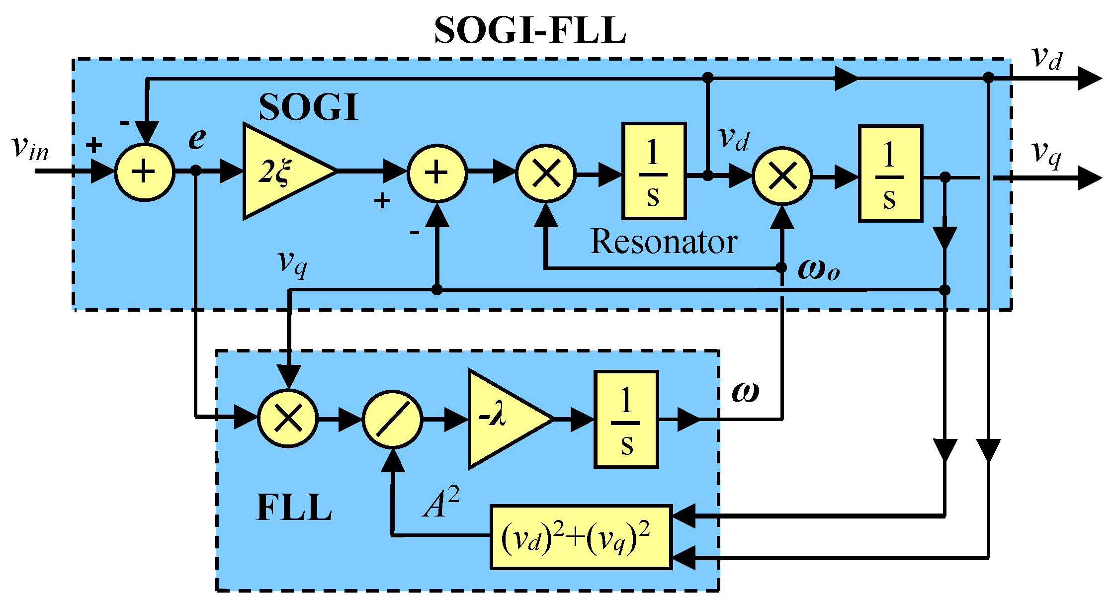
2. SOGI-FLL Response to Voltage Sags

The structure of the SOGI-FLL is shown in Figure 1, where ${\mathrm{v}}_{\mathrm{in}}$ is the input grid voltage, ${\mathsf{\omega }}_{\mathrm{o}}$ is the center frequency of the SOGI filter, ${\mathrm{v}}_{\mathrm{d}}$ and ${\mathrm{v}}_{\mathrm{q}}$ are its in-phase and quadrature-phase outputs, and $\mathsf{\omega }$ is the FLL estimated grid frequency acting as the center frequency of the SOGI filter.

The SOGI has band-pass filter (BPF) behavior for ${\mathrm{v}}_{\mathrm{d}}$ and low-pass filter (LPF) behavior for ${\mathrm{v}}_{\mathrm{q}}$, with their transfer functions defined as [6]

$${\mathrm{H}}_{\mathrm{d}}\left(\mathrm{s}\right)=\frac{{\mathrm{v}}_{\mathrm{d}}\left(\mathrm{s}\right)}{{\mathrm{v}}_{\mathrm{in}}\left(\mathrm{s}\right)}=\frac{{2\mathsf{\xi }\mathsf{\omega }}_{\mathrm{o}}·\mathrm{s}}{{\mathrm{s}}^2{+2\mathsf{\xi }\mathsf{\omega }}_{\mathrm{o}}·{\mathrm{s}+\mathsf{\omega }}_{\mathrm{o}}^2},$$

(1)

$${\mathrm{H}}_{\mathrm{q}}\left(\mathrm{s}\right)=\frac{{\mathrm{v}}_{\mathrm{q}}\left(\mathrm{s}\right)}{{\mathrm{v}}_{\mathrm{in}}\left(\mathrm{s}\right)}=\frac{{2\mathsf{\xi }\mathsf{\omega }}_{\mathrm{o}}^2}{{\mathrm{s}}^2{+2\mathsf{\xi }\mathsf{\omega }}_{\mathrm{o}}·{\mathrm{s}+\mathsf{\omega }}_{\mathrm{o}}^2},$$

(2)

The linearized model of the SOGI-FLL at a quasi-locked operating point has second-order dynamic behavior to a frequency change, described in [2] as

$$\frac{\mathsf{\omega }\left(\mathrm{s}\right)}{{\mathsf{\omega }}_{\mathrm{g}}\left(\mathrm{s}\right)}=\frac{\mathsf{\lambda }/2}{{\mathrm{s}}^2{+\mathsf{\xi }\mathsf{\omega }}_{\mathrm{n}}·\mathrm{s}+\mathsf{\lambda }/2},$$

(3)

where ${\mathsf{\omega }}_{\mathrm{g}}$ is the grid frequency and ${\mathsf{\omega }}_{\mathrm{n}}$ is its nominal value.

As seen in (3), the transient response of the estimated frequency to a change in the grid frequency is determined by the system parameters, i.e., the SOGI filter damping factor $\mathsf{\xi }$ and the FLL gain $\mathsf{\lambda }$. These same parameters are responsible for the estimated frequency behavior under whatever input voltage condition, either nominal or perturbed. In particular, the frequency response is greatly distorted in the case of voltage sag faults, exhibiting high nonlinear oscillating peaks.

For SOGI-FLL normal operation, these parameters are designed according to an inherent trade-off between the rejection of harmonic distortion at the SOGI outputs (1)–(2) and the transient response to frequency step perturbation in the grid voltage (3). An optimal value for the rejection of harmonics was used in [2,3] by choosing $\mathsf{\xi }=0.707$ for the SOGI gain. Also, an optimal damping factor of $1/\sqrt{2}$ was recommended in [2] for the transient response to a frequency step perturbation. According to (3), this damping factor leads to FLL gain $\mathsf{\lambda }=0.28·{\mathsf{\omega }}_{\mathrm{n}}^2$, with ${\mathsf{\omega }}_{\mathrm{n}}=2\mathsf{\pi }·50$ rad/s.

The response of the SOGI-FLL to a voltage sag depends on the moment when the fault happens. When the faults take place at non-zero input voltage, they first induce in the estimated frequency a transient peak above the 50 Hz nominal level, followed by a second transient peak below 50 Hz (see Figure 2a). Conversely, when the faults happen only at zero crossing input voltage, they first produce a peak below 50 Hz, followed by another peak above 50 Hz (see Figure 2b).

In the following, the responses in Figure 2a,b will be referenced as type-a and type-b, respectively. Figure 2 shows the responses to different voltage sag depths, namely, 20%, 40%, 60%, 80%, and 90%. Type-a sags happen at 0.195 s, when the grid voltage amplitude is negative, and type-b sags happen at 0.2 s, when the grid voltage is at zero crossing. A type-a sag response is also produced for positive values of grid voltage. The SOGI-FLL parameters are $\mathsf{\xi }=0.707$ and $\mathsf{\lambda }=0.28·{\mathsf{\omega }}_{\mathrm{n}}^2$ (rad/s²).

As seen in Figure 2, type-a and -b voltage sags have a high impact on the estimated frequency that increases with the sag depth. Figure 3 shows the evolution of the peak-to-peak amplitude of the estimated frequency distortion with the depth of type-a (upper subplot) and type-b (lower subplot) sags. Note that in both cases the perturbation trend is nonlinear but increases with the sag depth. Also, it is worth mentioning that although type-b voltage sags induce higher distortion in the estimated frequency, their likelihood of occurrence is much lower than that of type-a faults.

In view of Figure 2, the SOGI-FLL performance could be improved by limiting the estimated frequency distortion, which would allow faster system recovery after the fault. A straightforward solution to achieve this could simply be to saturate the estimated frequency at the boundaries where continuous or unlimited time of operation is required in the grid network (49 Hz and 51 Hz, respectively, for European grid codes), which is explained next.

3. SOGI-FLL Approaches with Saturation and with FSM

3.1. SOGI-FLL with a Saturation Approach

The first approach to face the fault is simply the insertion of a saturation block at the output of the FLL in order to bound the frequency estimation to the 49–51 Hz band, see Figure 4.

Figure 5 shows the response to an 80% depth voltage sag for $\mathsf{\xi }=0.707$ and $\mathsf{\lambda }=0.28·{\mathsf{\omega }}_{\mathrm{n}}^2$ (rad/s²). Note in Figure 5 that the perturbation is limited by the saturation block and that the time involved in the transient response has also been reduced.

3.2. SOGI-FLL with an FSM Approach

The SOGI-FLL response can be further improved by adopting a finite state machine (FSM) for identifying different stages in the frequency response of the system. This approach allows for defining better parameters for each stage of the response, in order to reduce the distortion impact and improve the transient response. A total of five stages in the operation of the SOGI-FLL during the fault are identified for the definition of the FSM.

An FSM is normally used in the definition of automatic control actions for the control of a wide variety of systems. It is defined according to the states identified in the operative steps needed to perform a given process. The FSM evolves from one state to another according to the value of its inputs and outputs in a given moment [14,15].

Proper tuning of the SOGI-FLL parameters is the key point to optimize its response through each one of the possible stages in the face of a fault. The optimization objective consists of retained the system to normal conditions as soon as possible.

In this work, the operation of the SOGI-FLL during a fault is depicted in the FSM of Figure 6, in which the following five stages are defined.

3.2.1. State S1. Normal Operation

The FLL frequency is between the maximum (51 Hz) and minimum (49 Hz) bounds. The SOGI-FLL operates with nominal parameters, designed for obtaining a given estimated frequency behavior. In this work the nominal parameters are $\xi =0.707$ and $\lambda =0.28·{\omega }_n^2$ (rad/s²). In this state, the system is waiting for a fault event, and the FSM will not perform any action until a saturation bound is reached.

3.2.2. State S2. Down-Saturation

The FLL frequency is reduced below 49 Hz due to a fault event, and the FSM keeps the output frequency saturated to 49 Hz. Here, the $\mathsf{\xi }$ and $\mathsf{\lambda }$ parameters are changed to different values designed by a trial and error procedure, in order to minimize the duration of the SOGI-FLL time response.

3.2.3. State S3. Up-Saturation

The FLL frequency goes beyond 51 Hz due to a fault, and the FSM holds the output frequency as saturated to 51 Hz. The $\mathsf{\xi }$ and $\mathsf{\lambda }$ parameters are optimized in order to achieve a better transient response.

3.2.4. State S4. Up to Down Transient

The FSM moves from state S3 (up-saturation) to S4 when the FLL frequency is lower than or equal to 51 Hz. Once in S4, the FSM can transition to three different states: either to S2 (down-saturation) if the FLL frequency is reduced below 49 Hz, or to S3 (up-saturation) if the FLL frequency again exceeds 51 Hz, or to S1 (normal operation). The transition from S4 to S1 is decided by a counter ${\mathrm{T}}_{\mathrm{C}}$ which is activated whenever the FLL frequency enters a narrow ±0.02% band, named $∆$, around 50 Hz, i.e., between 50.1 Hz and 49.9 Hz. The counter Tc is reset if the FLL frequency leaves that band. Therefore, a return to normal state S1 is only produced if Tc reaches a given maximum value ${\mathrm{T}}_{{\mathrm{C}}_{\max }}$.

3.2.5. State S5. Down to Up Transient

S5 is reached from S2 (down-saturation) when the FLL frequency is greater than or equal to 49 Hz. Once in S5, the FSM can either go to S3 (up-saturation), or return back to S2 (down-saturation), or go to S1 (normal operation). The return mechanism to the S1 state is the same as that defined previously for S4. If ${\mathrm{T}}_{\mathrm{C}}>{\mathrm{T}}_{{\mathrm{C}}_{\max }}$, then the FSM returns to S1.

Figure 7 depicts an example of a usual response of the SOGI-FLL during a voltage sag. Note in this figure how the FSM goes from S1 to S3 when the voltage sag begins, and then transitions from S3 to S4, then to S2, then to S5, and finally returns to S1. It can be seen how at S5 the estimated frequency enters the boundary labeled as $2∆$. From this moment, the counter ${\mathrm{T}}_{\mathrm{C}}$ is started, and the FSM returns to normal state S1 when the maximum count $T_{C_{max}}$ is reached, i.e., when ${\mathrm{T}}_{\mathrm{C}}>{\mathrm{T}}_{{\mathrm{C}}_{\max }}$. Note that the checking of the return condition illustrated for a response entering the S5 state also applies to responses entering the S4 state; see the FSM diagram in Figure 6.

Figure 8 shows the transient responses to a 90% depth type-a voltage sag of the unsaturated (in blue) and the saturated (in red) SOGI-FLL and also of the FSM-based SOGI-FLL (in green).

During the fault, the FSM-based SOGI-FLL was operated with different $\mathsf{\xi }$ and $\mathsf{\lambda }$ gains for each state. The SOGI gain was optimized by a series of trial and error simulations for 90%, 80%, 60%, and 40% sag depths, and the parameter values are shown in the upper section of

Table 1. FSM-based SOGI-FLL parameters for 90% to 40% depth type-a and type-b voltage sags.

Parameter			State
Type-a	S1	S2	S3	S4	S5
λ90%	0.28	0.07	0.07	0.08	0.05
λ80%	0.28	0.11	0.11	0.1	0.07
λ60%	0.28	0.12	0.12	0.14	0.13
λ40%	0.28	0.2	0.2	0.22	0.19
ξ90%	0.707	0.8	0.8	0.8	0.8
ξ80%	0.707	0.75	0.75	0.75	0.75
ξ60%	0.707	0.65	0.65	0.65	0.65
ξ40%	0.707	0.55	0.55	0.55	0.55
Type-b	S1	S2	S3	S4	S5
λ90%	0.28	0.07	0.07	0.04	0.03
λ80%	0.28	0.11	0.11	0.1	0.034
λ60%	0.28	0.12	0.12	0.2	0.055
λ40%	0.28	0.2	0.2	0.3	0.08
ξ90%	0.707	0.75	0.75	0.75	0.75
ξ80%	0.707	0.7	0.7	0.7	0.7
ξ60%	0.707	0.6	0.6	0.6	0.6
ξ40%	0.707	0.5	0.5	0.5	0.5

(note that λ is expressed as a fraction of ${\omega }_n^2$).

The same procedure was carried out for voltage sags of type-b. The $\mathsf{\xi }$ and $\mathsf{\lambda }$ values are shown in the lower section of Table 1. Figure 9 shows the transient responses to a 90% sag of the SOGI-FLL (in blue), the saturated (in red) SOGI-FLL, and the FSM-based SOGI-FLL (in green) for this case. As shown in Figure 8, the FSM-based transient response returned to normal operation faster.

As can be seen in Table 1, for each state and each depth percentage of voltage sag, there is a progression in the values of $\mathsf{\xi }$ and $\mathsf{\lambda }$. In general, there is an increase in the value of $\mathsf{\lambda }$ as the voltage sag depth decreases, and $\mathsf{\xi }$ decreases as the sag depth decreases. This behavior allows for determining the sustained progression trend of the parameters with the several sag depths. To do that, the sag depth is determined as

$${\mathrm{x}=1-\mathrm{A}}_{\mathrm{pu}},$$

(4)

where ${\mathrm{A}}_{\mathrm{pu}}$ is the estimated peak voltage amplitude in pu (i.e., ${\mathrm{A}}_{\mathrm{pu}}=\mathrm{A}/{\mathrm{A}}_{\mathrm{n}}$, where ${\mathrm{A}}_{\mathrm{n}}=\sqrt{2}·230{\mathrm{V}}_{\mathrm{rms}}$ is the nominal grid voltage amplitude) and x is the voltage sag depth in pu. $\mathrm{A}$ is obtained by means of the quadrature outputs of the SOGI as (see Figure 1)

$${\mathrm{A}=(\mathrm{v}}_{\mathrm{d}}{}^2{+\mathrm{v}}_{\mathrm{q}}{}^2{)}^{1/2}.$$

(5)

Now, with (4) and (5), the equations presented in

Table 2. Equations expressing $\lambda$ as a function of the sag depth x for each of the FSM states and sag types.

State	λ = f(x) Equation
Type-a
S2 & S3	$\mathsf{\lambda }=-4.58x^3+9.37x^2-6.39x+1.57$
S4	$\mathsf{\lambda }=0.36x^2-0.74x+0.46$
S5	$\mathsf{\lambda }=0.09x^2-0.41x+0.34$
Type-b
S2 & S3	$\mathsf{\lambda }=-4.58x^3+9.37x^2-6.39x+1.57$
S4	$\mathsf{\lambda }=-0.09x^2-0.39x+0.47$
S5	$\mathsf{\lambda }=0.1x^2-0.23x+0.15$

can be used for obtaining the $\mathsf{\lambda }$ values for the cases of type-a and -b sags and for any depth ranging from 40% to 90%. In the case of $\mathsf{\xi }$, the relationship is simpler and only two equations are needed, one for type-a and another for type-b (see

Table 3. Equations expressing $\xi$ as a function of the sag depth x for each of the FSM states and sag types.

Sag Type	ξ = f(x) Equation
Type-a	$\xi =0.5x$ + 0.35
Type-b	$\xi =0.5x$ + 0.3

).

Figure 10 and Figure 11 show the results of using the equations of Table 2 and Table 3 to obtain $\mathsf{\xi }$ and $\mathsf{\lambda }$ parameters for type-a and -b sags and for 70% and 50% sag depths, respectively. Observe in Figure 10 and Figure 11 that the FSM-based SOGI-FLL response is less oscillatory and faster than the others, guaranteeing a smooth return to a normal state of operation.

The recovery times of the three SOGI-FLL schemes were obtained for different sag depths, as shown in

Table 4. Recovery times of the different SOGI-FLL schemes for various voltage sag depths.

Sag Depth	SOGI-FLL UNSAT(s)	SOGI-FLL SAT(s)	SOGI-FLL FSM(s)	% Reduction
90%	0.0439	0.0354	0.0150	66%
80%	0.0433	0.0349	0.0164	62%
70%	0.0422	0.0337	0.0213	50%
60%	0.0374	0.0324	0.0218	42%
50%	0.0360	0.0302	0.0227	37%
40%	0.0349	0.0271	0.0228	35%

. The percentage time reduction of the FSM scheme regarding the SOGI-FLL was also evaluated. Notice that the FSM-based method achieved better results for the deeper voltage sags.

4. FSM Modification for Grid Frequency Tracking and Response to Grid Harmonics

The FSM was initially designed and simulated working at a constant 50 Hz grid nominal frequency, with fixed saturation bounds at ±1 Hz relative to the nominal value (or ±2π rad/s). Therefore, the FSM could not work properly when the grid frequency is outside these boundaries. The FSM scheme was then modified to be able to track the grid frequency changes. The modification can be seen in Figure 12 and consists of including an LPF in the path supplying the estimated grid frequency ω to the FSM. The LPF is first-order and has the following transfer function:

$${\mathsf{\omega }}_{\mathrm{LPF}}\left(\mathrm{s}\right)=\frac{\mathrm{a}}{\mathrm{s}+\mathrm{a}}\mathsf{\omega }\left(\mathrm{s}\right),$$

(6)

where ${\omega }_{LPF}$ is the LPF output and $a=2\pi f_c$ is its cutoff frequency (rad/s).

The LPF was designed to have a low cutoff frequency with the purpose of achieving the average of the estimated frequency, i.e.,

$${\mathsf{\omega }}_{\mathrm{LPF}}\left(\mathrm{t}\right)=⟨\mathsf{\omega }\left(\mathrm{t}\right)⟩,$$

(7)

where <–> denotes the average. Then, the LPF transient response is slow and serves as an analog memory of the value that the estimated grid frequency ω had just before the fault event. The ${\mathsf{\omega }}_{\mathrm{LPF}}$ signal was introduced as a new input to the FSM and is used for defining the saturation bound levels, which are now variable. The saturation bounds are determined during normal operation of the FSM, at state S1, and are defined as

$${\mathsf{\omega }}_{{\mathrm{SAT}}_{\mathrm{up}}}{=\mathsf{\omega }}_{\mathrm{LPF}}+2\mathsf{\pi },$$

(8)

$${\mathsf{\omega }}_{{\mathrm{SAT}}_{\mathrm{down}}}{=\mathsf{\omega }}_{\mathrm{LPF}}-2\mathsf{\pi },.$$

(9)

where ${\mathsf{\omega }}_{{\mathrm{SAT}}_{\mathrm{up}}}$. and ${\mathsf{\omega }}_{{\mathrm{SAT}}_{\mathrm{down}}}$ are the FSM upper and lower saturation bounds (rad/s).

The functioning of (8), (9) can be well understood using the time response depicted in Figure 13, which shows the FSM and ${\mathsf{\omega }}_{\mathrm{LPF}}$ transient responses to an 80% depth voltage sag happening at t = 0.195 s. The LPF had a cutoff frequency of ${\mathsf{\omega }}_{\mathrm{c}}=10\mathsf{\pi }$ rad/s.

In Figure 13, it can be seen how $\mathsf{\omega }$ very quickly reaches the upper saturation bound ${\mathsf{\omega }}_{{\mathrm{SAT}}_{\mathrm{up}}}$ at the end of the time interval from 0.1950 s to 0.1964 s, during which the FSM is in the S1 normal operation state. At this point (t = 0.1964 s), $\mathsf{\omega }={\mathsf{\omega }}_{{\mathrm{SAT}}_{\mathrm{up}}}$ and the FSM state changes from S1 to S3. It is also at this moment that the value of ${\mathsf{\omega }}_{\mathrm{LPF}}$ is stored in an inner memory variable named ${\mathsf{\omega }}_{{\mathrm{LPF}}_{\mathrm{Mem}}}$ for later use. Then, ${\mathsf{\omega }}_{{\mathrm{LPF}}_{\mathrm{Mem}}}$ is defined as

$${\mathsf{\omega }}_{{\mathrm{LPF}}_{\mathrm{Mem}}}{=\mathsf{\omega }}_{{\mathrm{LPF}}_{{|\mathsf{\omega }=\mathsf{\omega }}_{{\mathrm{SAT}}_{\mathrm{up}}}}},$$

(10)

According to Figure 13, ${\mathsf{\omega }}_{{\mathrm{LPF}}_{\mathrm{Mem}}}=2\mathsf{\pi }·50.019$ rad/s and ${\mathsf{\omega }}_{{\mathrm{SAT}}_{\mathrm{up}}}={\mathsf{\omega }}_{{\mathrm{LPF}}_{\mathrm{Mem}}}+2\mathsf{\pi }=2\mathsf{\pi }·51.019$ rad/s. Note that ${\mathsf{\omega }}_{{\mathrm{LPF}}_{\mathrm{Mem}}}$ is slightly away from the nominal $2\mathsf{\pi }·$ 50 rad/s value, which supposes that ${\mathsf{\omega }}_{{\mathrm{SAT}}_{\mathrm{up}}}$ is a little bit displaced from the ideal value of $2\mathsf{\pi }$·51 rad/s. However, the effect over the behavior of $\mathsf{\omega }$ is negligible.

Consequently, the fixed upper 51 Hz and lower 49 Hz saturation bounds employed in Figure 6 are replaced by the new saturation variables ${\mathrm{SAT}}_{\mathrm{up}}$ and ${\mathrm{SAT}}_{\mathrm{down}}$ determined by (8) and (9), respectively, which are stored in inner variables.

Moreover, the return of the FSM to the normal operating conditions state S1, defined in Figure 6 for the transitions from S4 to S1 and from S5 to S1, has also changed. Now, ${\mathsf{\omega }}_{{\mathrm{LPF}}_{\mathrm{Mem}}}$ is used instead of ${\mathsf{\omega }}_n$ as center of the $\pm ∆=\pm 0.02\%$ narrow band, i.e.,

$${\mathsf{\omega }}_{{\mathrm{LPF}}_{\mathrm{Mem}}}-∆\le \mathsf{\omega }\le {\mathsf{\omega }}_{{\mathrm{LPF}}_{\mathrm{Mem}}}+∆,$$

(11)

Then, when $\mathsf{\omega }$ is confined within these bounds, the ${\mathrm{T}}_{\mathrm{C}}$ counter is started and the return to S1 is decided if ${\mathrm{T}}_{\mathrm{C}}\ge {\mathrm{T}}_{{\mathrm{C}}_{\mathrm{Max}}}$. The counter ${\mathrm{T}}_{\mathrm{C}}$ is reset when $\mathsf{\omega }$ leaves the band, which can happen due to unexpected interference or to the presence of huge levels of harmonic distortion in the grid. Otherwise, in normal conditions, $\mathsf{\omega }$ progressively stabilizes, the counter ${\mathrm{T}}_{\mathrm{C}}$ starts to count when condition (11) is met, and the FSM returns to state S1 when ${\mathrm{T}}_{\mathrm{C}}\ge {\mathrm{T}}_{{\mathrm{C}}_{\mathrm{Max}}}$. The value of ${\mathrm{T}}_{{\mathrm{C}}_{\mathrm{Max}}}$ can be set to adjust the time needed to return to the normal operation state once the band $2$Δ has been reached. Upon return to state S1, the integrator of the LPF is initialized to the actual grid frequency, i.e., ${\mathsf{\omega }}_{\mathrm{LPF}}=\mathsf{\omega }$ (see Figure 13c), which supposes that the system is ready again to face a new fault.

Finally, Figure 14 depicts the results obtained when considering three different scenarios which have in common the occurrence of an 80% depth voltage sag at $t=0.22s$. In the first scenario, the grid frequency goes from 50 Hz to 50.5 Hz at $t=0.15s$ (blue line), while it remains at 50 Hz in the second scenario (red line) and goes down to 49.5 Hz also at $t=0.22s$ in the third scenario (green line). It can be seen how the FSM algorithm is able to follow the step frequency changes and the voltage sags properly. Also, the FSM keeps a saturation band of $\pm 1$ Hz on the grid frequency.

The same modification explained in this section for tracking the grid frequency changes allows the system to respond to faults happening in grid networks distorted by harmonics. Figure 15 shows the behavior of $\mathsf{\omega }$ and ${\mathsf{\omega }}_{\mathrm{LPF}}$ when an 80% depth voltage sag takes place at t = 0.195 s in a grid distorted by a 5th harmonic with 3% amplitude.

It can be seen in Figure 15 how the FSM can work properly with the distorted grid voltage. The condition for being able to handle harmonic distortion is that the peak-to-peak amplitude ${∆}_{\mathsf{\omega }}$ of the distortion in the grid frequency should be less than the boundary width, i.e.,

$${∆}_{\mathsf{\omega }}<2∆,$$

(12)

Then, the setting of the value for the boundary $2∆$ should take into consideration the maximum harmonic distortion that the FSM has to face. Also, a proper value for ${\mathrm{T}}_{{\mathrm{C}}_{\mathrm{Max}}}$ should be chosen to determine a reasonable time for returning the state of the FSM to S1.

5. Swell Fault and Short Transient Response Capability

Figure 16 depicts the response of the SOGI-FLL to voltage swell perturbations ranging from 1.1 pu to 1.8 pu, with optimal parameters $\mathsf{\xi }=0.707$ and $\mathsf{\lambda }=0.28·{\mathsf{\omega }}_{\mathrm{n}}^2$ rad/s². This figure shows that swell perturbations have a different distortion impact than voltage sags on the SOGI-FLL estimated frequency.

Notice in Figure 16 that for swells happening at non-zero input voltage moments (type-a), the perturbations almost do not reach the $\pm 1\mathrm{Hz}$ saturation bounds in almost all cases. So, for type-a swells, the FSM will not act. However, for swells happening at zero voltage (type-b), the perturbations surpass the established $\pm 1\mathrm{Hz}$ bounds for fault levels ranging from 1.3 pu to 1.8 pu, and the FSM can be applied to these cases to improve the response.

In conclusion, for type-b swells ranging from 1.3 pu to 1.8 pu, $\mathsf{\omega }$ will reach ${\mathrm{SAT}}_{\mathrm{up}}$ and the FSM can be applied in the same way that it was applied for voltage sags, provided that the variable $\mathrm{x}$ defined in (4) is appropriately modified. For instance, a 1.3 pu swell can be treated by the FSM like a voltage sag of 30% depth if the variable $\mathrm{x}$ is set to $\mathrm{x}=0.3$ pu. In the same way, a 1.8 pu swell can be treated by the FSM as a sag having $\mathrm{x}=0.8$, or 80% depth. Therefore, the FSM can be applied to voltage sags and swells in the same way by using the following relation instead of (4):

$$\mathrm{x}=1-\mathrm{abs}\left({\mathrm{A}}_{\mathrm{y}}{-\mathrm{A}}_{\mathrm{pu}}\right),$$

(13)

where ${\mathrm{A}}_{\mathrm{y}}=0$ holds for voltage sags and ${\mathrm{A}}_{\mathrm{y}}=2$ for voltage swells, and abs(–) represents the absolute value function. The block diagram depicted in Figure 17 clarifies this issue well and is used in the algorithm to differentiate a voltage sag from a voltage swell.

The FSM from here on incorporates the algorithm of Figure 17 and uses Equation (13) to respond in the same way to voltage sags or swells.

Figure 18 illustrates the response of the SOGI-FLL-FSM to several voltage swells (Figure 18a,b) and sags (Figure 18c,d) with different durations. Fault events in Figure 18a,c extend for four cycles, while those in Figure 18b,d do so for two cycles, which correspond to the shorter event duration that does not result in overlapped transients at the beginning and at the end of the faults. As fault transients, we consider here the event of a voltage swell or sag and recovery to nominal grid voltage in a short time.

In Figure 18a,b, the swells rise to 1.8 pu and then return to 1 pu. In Figure 18c,d, the sags go down to 0.2 pu and then return to 1 pu. Notice in these figures that the FSM can respond well to both type of faults, which can improve the capability to respond to short-time-duration transients.

Finally, the SOGI-FLL-FSM response to the same voltage sag as that in Figure 18d is shown in Figure 19 when the grid voltage is affected by a 5th harmonic distortion with 4% amplitude. Notice in this figure that the response is similar to that achieved in Figure 18d, but in this case the harmonic distortion is reflected in the estimated frequency response.

6. Discussion

In this paper we aimed to improve the response of the SOGI-FLL to voltage sags since it is highly sensitive to this kind of fault. We first showed the scope of this problem for a given set of gain parameters. Then, we proposed a simple solution by using a saturation block placed after the FLL integrator to limit the frequency response to the grid operating bounds of 51 Hz and 49 Hz. After that, we proposed an FSM as a way to operate with different SOGI-FLL gains through the pattern developed by the system frequency response to the fault. A set of five stages was identified in the frequency response of the SOGI-FLL to a voltage sag fault. These stages were used to construct an FSM algorithm. The FSM was designed to work on two types of patterns that were identified in the frequency response: type-a and type-b patterns, caused by faults happening at no zero crossing and at zero crossing of the grid voltage, respectively. The FSM allows for defining different SOGI-FLL gains for the different FSM states, according to the fault pattern. The response of the SOGI-FLL was then optimized by a series of trial and error simulations in order to achieve the best responses to given voltage sags with depths ranging from 40% to 90%. Analytical functions relating the system parameters to the sag depths were fitted to the gains obtained by this procedure, facilitating operation with any voltage sag depth. Finally, simulations proved the feasibility of this method that improves the response of the SOGI-FLL to voltage sags and reduces the recovery time involved in the transient perturbation. Moreover, an LPF was incorporated into the defined FSM in order to track the grid frequency changes, including harmonic distortion. Finally, the FSM was also applied to voltage swells, showing that it is able to handle both kind of faults: sags and swells. More research should be performed in order to reduce the number of stages of the FSM and simplify the overall structure. Further research should be performed regarding several aspects, such as applying more elaborate tuning methods for the SOGI-FLL-FSM, which is a nontrivial task due to the increased nonlinearity introduced by the saturation and the highly transient nature of the analyzed sag and swell perturbations. Research should also be performed regarding the introduction of the error signal of the SOGI structure into the FSM algorithm in order to accelerate the response to a fault and reduce the time response. Moreover, the FSM idea can be applied to other grid monitoring approaches and its performance assessed compared with the actual approach.

References

1. Teodorescu, R.; Liserre, M.; Rodriguez, P. Grid Converters for Photovoltaic and Wind Power Systems; John Wiley & Sons: Hoboken, NJ, USA, 2011; Volume 29. [Google Scholar]
2. Golestan, S.; Ebrahimzadeh, E.; Guerrero, J.M.; Vasquez, J.C. An adaptive resonant regulator for single-phase grid-tied VSCs. IEEE Trans. Power Electron. 2018, 33, 1867–1873. [Google Scholar] [CrossRef]
3. Rodríguez, P.; Luna, A.; Candela, I.; Mujal, R.; Teodorescu, R.; Blaabjerg, F. Multiresonant frequency-locked loop for grid synchronization of power converters under distorted grid conditions. IEEE Trans. Ind. Electron. 2011, 58, 127–138. [Google Scholar] [CrossRef] [Green Version]
4. Matas Alcalá, J.; Martín Cañadas, M.E.; El Mariachet Carreño, J.; Abusorrah, A.; Al-Turki, Y.A. A new LPF-based grid frequency estimation for the SOGI filter with improved harmonic rejection. In Renewable Energy and Power Quality Journal (RE&PQJ); UPCommons: Salamanca, Spain, 2018. [Google Scholar]
5. Ye, S. Fuzzy sliding mode observer with dual SOGI-FLL in sensorless control of PMSM drives. ISA Trans. 2019, 85, 161–176. [Google Scholar] [CrossRef] [PubMed]
6. Ngo, T.; Nguyen, Q.; Santoso, S. Improving performance of single-phase SOGI-FLL under DC-offset voltage condition. In Proceedings of the IECON 2014-40th Annual Conference of the IEEE Industrial Electronics Society, Dallas, TX, USA, 29 October–1 November 2014. [Google Scholar]
7. Park, S.J.; Nguyen, T.H.; Lee, D.-C. Advanced SOGI-FLL scheme based on fuzzy logic for single-phase grid-connected converters. J. Power Electron. 2014, 14, 598–607. [Google Scholar] [CrossRef] [Green Version]
8. Kang, J.W.; Shin, K.W.; Lee, H.; Kang, K.M.; Kim, J.; Won, C.Y. A Study on Stability Control of Grid Connected DC Distribution System Based on Second Order Generalized Integrator-Frequency Locked Loop (SOGI-FLL). Appl. Sci. 2018, 8, 1387. [Google Scholar] [CrossRef] [Green Version]
9. Matas, J.; Martin, H.; de la Hoz, J.; Abusorrah, A.; Al-Turki, Y.A.; Al-Hindawi, M. A family of gradient descent grid frequency estimators for the SOGI filter. IEEE Trans. Power Electron. 2018, 33, 5796–5810. [Google Scholar] [CrossRef]
10. Cao, W.; Liu, K.; Kang, H.; Wang, S.; Fan, D.; Zhao, J. Resonance Detection Strategy for Multi-Parallel Inverter-Based Grid-Connected Renewable Power System Using Cascaded SOGI-FLL. Sustainability 2019, 11, 4839. [Google Scholar] [CrossRef] [Green Version]
11. Kim, B.J.; Kum, H.J.; Park, J.M.; Won, C.Y. Analysis, Design and Implementation of Droop-Controlled Parallel-Inverters Using Dynamic Phasor Model and SOGI-FLL in Microgrid Applications. Energies 2018, 11, 1683. [Google Scholar] [CrossRef] [Green Version]
12. Matas, J.; Castilla, M.; Miret, J.; de Vicuña, L.G.; Guzman, R. An adaptive prefiltering method to improve the speed/accuracy tradeoff of voltage sequence detection methods under adverse grid conditions. IEEE Trans. Ind. Electron. 2014, 61, 2139–2151. [Google Scholar] [CrossRef]
13. Huang, Z.; Bian, L. A Differential Resonant Voltage Sensor Consisting of Piezo Bimorph and Quartz Crystal Double-ended Tuning Fork Resonators. Sensors 2019, 19, 5031. [Google Scholar] [CrossRef] [Green Version]
14. Hong, P.; Turk, M.; Huang, T.S. Gesture modeling and recognition using finite state machines. In Proceedings of the Fourth IEEE International Conference on Automatic Face and Gesture Recognition (Cat. No. PR00580), Grenoble, France, 28–30 March 2000. [Google Scholar]
15. Benini, L.; De Micheli, G.; Vermeulen, F. Finite-state machine partitioning for low power. In Proceedings of the 1999 IEEE International Symposium on Circuits and Systems (ISCAS), Orlando, FL, USA, 30 May–2 June 1998. [Google Scholar]
16. El Mariachet, J.; Matas, J.; Martín, H.; Li, M.; Guan, Y.; Guerrero, J.M. A Power Calculation Algorithm for Single-Phase Droop-Operated-Inverters Considering Linear and Nonlinear Loads HIL-Assessed. Electronics 2019, 8, 1366. [Google Scholar] [CrossRef] [Green Version]
17. Matas, J.; Martin, H.; De La Hoz, J.; Abusorrah, A.; Al-Turki, Y.A.; Alshaeikh, H. A New THD Measurement Method with Small Computational Burden Using a SOGI-FLL Grid Monitoring System. IEEE Trans. Power Electron. 2020, 35, 5797–5811. [Google Scholar] [CrossRef]
18. Naidoo, R.; Pillay, P. A new method of voltage sag and swell detection. IEEE Trans. Power Deliv. 2007, 22, 1056–1063. [Google Scholar] [CrossRef]
19. Yunus, A.S.; Masoum, M.A.; Abu-Siada, A. Application of SMES to enhance the dynamic performance of DFIG during voltage sag and swell. IEEE Trans. Appl. Supercond. 2012, 22, 5702009. [Google Scholar] [CrossRef]
20. Popavath, L.N.; Kaliannan, P. Photovoltaic-STATCOM with low voltage ride through strategy and power quality enhancement in a grid integrated wind-PV system. Electronics 2018, 7, 51. [Google Scholar] [CrossRef] [Green Version]
21. Bai, H. Position Estimation of a PMSM in an Electric Propulsion Ship System Based on High-Frequency Injection. Electronics 2020, 9, 276. [Google Scholar] [CrossRef] [Green Version]
22. Zeb, K.; Islam, S.U.; Din, W.U.; Khan, I.; Ishfaq, M.; Busarello, T.D.C.; Ahmad, I.; Kim, H.J. Design of Fuzzy-PI and Fuzzy-Sliding Mode Controllers for Single-Phase Two-Stages Grid-Connected Transformerless Photovoltaic Inverter. Electronics 2019, 8, 520. [Google Scholar] [CrossRef] [Green Version]
23. Du, H.; Sun, Q.; Cheng, Q.; Ma, D.; Wang, X. An Adaptive Frequency Phase-Locked Loop Based on a Third Order Generalized Integrator. Energies 2019, 12, 309. [Google Scholar] [CrossRef] [Green Version]
24. Filipović, F.; Petronijević, M.; Mitrović, N.; Banković, B.; Kostić, V. A Novel Repetitive Control Enhanced Phase-Locked Loop for Synchronization of Three-Phase Grid-Connected Converters. Energies 2020, 13, 135. [Google Scholar] [CrossRef] [Green Version]
25. Rey-Boué, A.B.; Guerrero-Rodríguez, N.F.; Stöckl, J.; Strasser, T.I. Modeling and Design of the Vector Control for a Three-Phase Single-Stage Grid-Connected PV System with LVRT Capability according to the Spanish Grid Code. Energies 2019, 12, 2899. [Google Scholar] [CrossRef] [Green Version]
26. Doget, T.; Etien, E.; Rambault, L.; Cauet, S. A PLL-Based Online Estimation of Induction Motor Consumption Without Electrical Measurement. Electronics 2019, 8, 469. [Google Scholar] [CrossRef] [Green Version]
27. Sun, Y.; de Jong, E.C.W.; Wang, X.; Yang, D.; Blaabjerg, F.; Cuk, V.; Cobben, J.F.G. The Impact of PLL Dynamics on the Low Inertia Power Grid: A Case Study of Bonaire Island Power System. Energies 2019, 12, 1259. [Google Scholar] [CrossRef] [Green Version]
Figure 1. Block diagram structure of the Second-Order Generalized Integrator–Frequency-Locked Loop (SOGI-FLL) filter.
Electronics 09 00612 g001
Figure 2. Perturbations induced in the SOGI-FLL estimated frequency for different voltage sag depths: (a) at non-zero input voltage; (b) at zero crossing input voltage.
Electronics 09 00612 g002
Figure 3. Evolution of the peak-to-peak amplitude of the estimated frequency distortion with the sag depth. Upper: type-a sag. Lower: type-b sag.
Electronics 09 00612 g003
Figure 4. FLL with a saturation block.
Electronics 09 00612 g004
Figure 5. SOGI-FLL response to an 80% depth type-a voltage sag. In blue: without a saturation block. In red: with a saturation block.
Electronics 09 00612 g005
Figure 6. Proposed finite state machine (FSM) for the SOGI-FLL.
Electronics 09 00612 g006
Figure 7. Example of FSM evolution during a voltage sag.
Electronics 09 00612 g007
Figure 8. Transient responses to a 90% depth type-a voltage sag. In blue: SOGI-FLL. In red: SOGI-FLL with saturation. In green: FSM-based SOGI-FLL.
Electronics 09 00612 g008
Figure 9. Transient response to a 90% depth type-b voltage sag. In blue: unsaturated SOGI-FLL. In red: SOGI-FLL with saturation. In green: FSM-based SOGI-FLL.
Electronics 09 00612 g009
Figure 10. Transient responses to a 70% sag depth using the equations of Table 2 and Table 3 to obtain ξ and λ . In blue: SOGI-FLL. In red: SOGI-FLL with saturation. In green: FSM-based SOGI-FLL Upper: type-a sag. Lower: type-b sag.
Electronics 09 00612 g010
Figure 11. Transient responses to a 50% sag depth using the equations of Table 2 and Table 3 to obtain ξ and λ . In blue: unsaturated SOGI-FLL. In red: SOGI-FLL with saturation. In green: FSM-based SOGI-FLL Upper: type-a sag. Down: type-b sag.
Electronics 09 00612 g011
Figure 12. Block diagram structure of the SOGI-FLL-FSM including a low-pass filter (LPF) for tracking the grid frequency.
Electronics 09 00612 g012
Figure 13. Estimated grid frequency ω and its average value ω L P F transient responses to an 80% depth voltage sag happening at t = 0.195 s. (a) ω and ω LPF transient responses. (b,c) Transient details.
Electronics 09 00612 g013
Figure 14. Estimated frequency transient responses to 80% depth voltage sags produced at different grid frequency values. In blue: ω g = 50.5   Hz. In red: ω g = 50   Hz. In green: ω g = 49.5   Hz.
Electronics 09 00612 g014
Figure 15. ω and ω LPF transient responses to an 80% depth voltage sag happening at t = 0.195 s for a grid voltage distorted by a 5th harmonic with 3% amplitude.
Electronics 09 00612 g015
Figure 16. Perturbations induced in the SOGI-FLL estimated frequency for different voltage swell levels. Upper: at non-zero input voltage. Lower: at zero crossing input voltage.
Electronics 09 00612 g016
Figure 17. Algorithm used for differentiating voltage sags from voltage swells.
Electronics 09 00612 g017
Figure 18. Response of the SOGI-FLL-FSM to short-duration voltage swells and sags. (a,b): 1.8 pu swells at 0.2 s with four and two cycles duration, respectively. (c,d): 0.2 pu sags at 0.2 s with four and two cycles duration, respectively.
Electronics 09 00612 g018aElectronics 09 00612 g018b
Figure 19. Response of the SOGI-FLL-FSM to a two-cycle 0.2 pu voltage sag at 0.2 s in the presence of a 5th harmonic with 4% amplitude in the grid voltage.
Electronics 09 00612 g019