Abstract
With the higher penetration of renewable energy, the influence of grid equivalent distribution cable impedance on grid-connected inverter stability is attracting increasing attention. In order to suppress the interaction between grid distribution cable impedance and output impedance of the grid-connected system, the active damping strategy is often used. When a capacitive current loop is used, the damping coefficient increases with the grid impedance increasing. However, the excessive damping coefficient will cause the unstable operation of the system. In order to enhance the robustness of the system, a novel control strategy which is suitable for wide-range grid impedance variation is proposed. In this strategy, the capacitor current inner loop is combined with the grid current inner loop, and grid voltage feedforward is included. Since the virtual impedance, active damping and voltage feed-forward are normalized, the changing tendency of the damping coefficient of the grid-current inner loop is opposite to that of capacitor current inner-loop. The overall damping coefficient of the system remains relatively constant when the grid impedance changes, and this effectively suppresses the resonance of the system. In this paper, the method is analyzed and the parameters are designed and optimized. Finally, the simulation and experiment are presented to verify the analysis.
1. Introduction
With the aggravation of the global energy crisis, the development and utilization of renewable energy is especially important [1]. The higher penetration and position uncertainty of independent distributed generation systems mean that the grid-connected inverter distribution cable cannot be ignored. Moreover, the increase in non-linear load makes the grid contain a large number of background harmonics which are no longer ideal a voltage source. These two principal reasons lead to a weak grid. The effect of the interaction between the distribution cable impedance and the output impedance of the inverter on the grid current quality can no longer be ignored in a weak grid. In a broad sense, the grid impedance should be defined as the equivalent impedance of the grid. The traditional grid impedance only includes the impedance of transmission lines and the impedance of the transmission equipment. Moreover, the equivalent impedance of power grid also includes the equivalent output impedance of power generation equipment in distributed generation system, which is equivalent to the impedance of the grid side. The grid impedance varies according to the geographic location of the power generation equipment; the change in penetration will also cause changes in the equivalent impedance of the power grid while the geographic location of the power generation equipment is fixed. Therefore, the equivalent impedance of the grid will change when the penetration of the grid-connected renewable power generation changes, so that the system may resonate. Therefore, it is of great significance to study the control strategy suitable for wide-range grid impedance variation.
An LCL filter is a T-filter network, composed of inductance and capacitance. It has stronger ability to suppress the high frequency components of current, but it has resonance peaks, which easily lead the system to oscillate [2]. At present, the active damping method [3,4] or effective control of cut-off frequency [5,6,7,8] is commonly used to suppress resonance. The LCL virtual damping with physical meaning corresponding to different state feedbacks was studied in [9,10]. It adopts inverter-side current closed-loop to achieve damping in [11]. However, none of the above control schemes can adapt to the change in grid impedance under weak grid conditions.
Scholars have proposed various control schemes for the problem of a weak grid, including series virtual impedance [12], phase compensation [13,14], and robust control [15,16,17,18]. In [12], a series-parallel virtual impedance setting scheme was proposed to overcome the disadvantage that the capacitive current closed-loop virtual impedance method suppress the stability of the system with the increase in grid impedance. In [13], the conclusion was drawn that the phase margin of the system decreases gradually with the increase in grid impedance under weak grid conditions. In addition, the lead-lag compensation function is obtained to compensate the phase of system by measuring grid impedance on-line. In [14], the relationship between virtual impedance of capacitor current inner-loop and lead-lag compensation function was analyzed, then the lead-lag compensation control function was proposed, but the value of grid impedance should be known, which is a very important premise. [18,19] used robust control to design the controller directly according to the performance of the inverters, taking grid impedance into account. However, this control scheme requires a lot of variables to be collected and the calculation is complicated. In [20], The stability of voltage feedforward and current decoupling system in weak grid is analyzed by complex vector. The system stability is related to the grid impedance, so the control scheme needs to be improved. The above control strategies for weak power grids has the disadvantages of complex control and difficulty in accurately obtaining grid impedance on-line. Therefore, these strategies cannot adapt to the wide range variation of grid impedance.
The analysis shows that when a capacitive current loop is used to increase the system damping coefficient, the damping coefficient increases with the grid impedance increasing. Moreover, the excessive damping coefficient will lead to the second-order damping system becoming two first-order inertia links, thus reducing the phase margin of the system. In [21,22,23], the grid-current inner loop is used as the active damping; due to the damping coefficient varying with the grid impedance, the robustness is poor.
In addition to the guaranteed stability properties, the goal of the closed-loop control of grid-connected inverters also needs to take harmonic suppression and grid interference suppression into account. At present, there are two main schemes to suppress grid background harmonics: improving the outer-loop controller and adding additional loops. Nowadays, improving the outer-loop controller commonly uses harmonic quasi proportional integral resonance controller (H-QPIR) and harmonic quasi proportional complex integral controller (H-QPCI) with phase compensation function. Adding additional loops is mainly used to suppress grid interference by adding a circuit related to grid voltage. In [24,25], full voltage feed-forward is obtained from the closed-loop transfer function. However, full voltage feed-forward contains differential items which are easy to generate interference, so only proportional feed-forward is generally used. Of course, scholars have also put forward many improved control schemes for voltage feed-forward.
According to the above, in order to make the control system suitable for wide range variation of grid impedance and able suppress the grid background harmonics, in this paper, through parameter design, the damping coefficient of the grid-current closed loop decreases with the increase in the grid impedance. In addition, the trend is opposite to the change in the damping coefficient of the capacitor current inner-loop. At the same time, the grid voltage proportion feedforward is included, thus effectively suppressing the impact on the system, which is caused by the change in the equivalent impedance of the power grid. This control strategy is certainly creative.
The first part of this paper analyzes the new problems under weak grid conditions which exist in the current closed-loop control of grid based on active damping of capacitor current feedback; in the second part, a normalized active damping control strategy is proposed; in the third part, the parameters of the proposed control scheme are designed; in the fourth part, the correctness and effectiveness of the proposed control strategy and the obtained parameters are verified by simulation and experiment; and in the fifth part, the conclusions are drawn.
2. Closed-Loop Control of Grid Current Based on Capacitor Current Feedback Active Damping (Scheme 1)
The three-phase grid-connected inverter is transformed to α-β frame through coordinate transformation. Figure 1 is the structure diagram of α-axis equivalent system. The figure is composed of two parts: the main circuit and the control circuit. When grid impedance contains resistance components, it is beneficial to the stability of the system. In order to analyze the worst case, pure inductance is selected as the grid impedance in this paper. Hc(s) is the feedback coefficient of capacitor current inner loop, Gc(s) is the control compensator of grid current loop, and Gfd(s) is the feed-forward coefficient. Vdc is the DC bus voltage, ug is the AC grid line voltage, and Lg is the grid inductance.
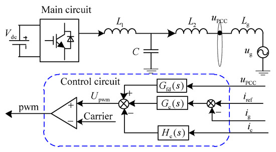
Figure 1.
Closed-loop system of grid-connected inverter with Scheme 1.
Scheme 1 selects the capacitive current loop as LCL filter damping. In order to suppress the grid harmonics, the following two control strategies can be considered to suppress the grid background harmonics.
Case 1: Adding the full feed-forward control of grid voltage [23], then the interference of grid voltage could be eliminated, but in full feed-forward control, only proportional feed-forward is usually used because of the existence of differential;
Case2: Add a harmonic controller to the outer-loop controller Gc(s) to achieve an infinite open-loop gain at the specified sub-harmonic, thereby suppressing the harmonic current.
The mathematical model corresponding to Figure 1 can be obtained.
The open-loop transfer function can be obtained from Figure 2 [26].
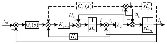
Figure 2.
System equivalent block diagram of Figure 1.
Kpwm is the amplification factor of the power-switching device, which is related to the input DC-voltage and the amplitude of the modulation wave. Kpwm is 400 in this paper.
When considering the suppression of background harmonics, it is known from the above analysis that the voltage feedforward and harmonic controller can choose one of them. Therefore, when selecting voltage proportional feed-forward, Gh(s) = 0, and when choosing harmonic controller, Gfd(s) = 0. Set the LCL filter parameters in this paper as: L1 = 4 mH; L2 = 2 mH; C = 6 × 10⁻⁶ μF [27].
In order to simplify the calculation, no matter which method is adopted to suppress the grid background harmonic, the outer loop controller could be designed according to the proportional integral (PI) controller.
Case 1: Adding the full feed-forward control of grid voltage is selected to suppress the background harmonics, the outer loop is the fundamental quasi proportional integral resonance (QPIR). At the fundamental frequency, this controller can provide a larger open-loop gain compared with the PI controller, thus reducing the steady-state tracking error of the system. Then, the amplitude and phase of both controllers are basically the same at the cut-off frequency and the harmonic frequency, which does not affect the stability of the system.
Case 2: When H-QPIR is selected to suppress background harmonics, the outer-loop controller Gc(s) contains the harmonic controller. Compared with the Bode diagram of open-loop transfer function with PI controller as outer loop, the amplitude curve of this controller moves up as a whole. By adjusting the Bode diagram, the Kp corresponding to the same cut-off frequency as a PI controller can be obtained. In medium and high frequency bands (ω > 7ω0), PI controllers can be equivalent to proportional controllers.
The typical second-order model can be used to design regulator parameters. In order to obtain the optimal static and dynamic characteristics under strong grid conditions, the parameters are calculated according to Lg = 0 mH. As the length of this article is limited and Scheme 1 is not the focus of this paper, only the design parameters are given: Hc = 0.144; ωc = 1.5;
Case 1: When voltage feed-forward control is adopted to suppress grid background harmonics, Kp = 0.052 and Kr = 10.8 are the values of the outer-loop control compensator Gc(s);
Case 2: When the harmonic control compensator is used to suppress the grid background harmonics, Kp = 0.035 and Kr = 7.3 are the values of the outer-loop control compensator Gc(s).
The open-loop Bode diagram with different grid impedances in both cases of Scheme 1 are given in Figure 3 and Figure 4.
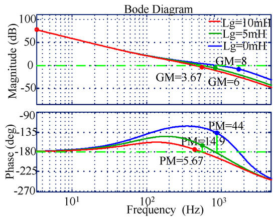
Figure 3.
Open-loop transfer function Bode diagram using the approach of proportional voltage feed-forward.
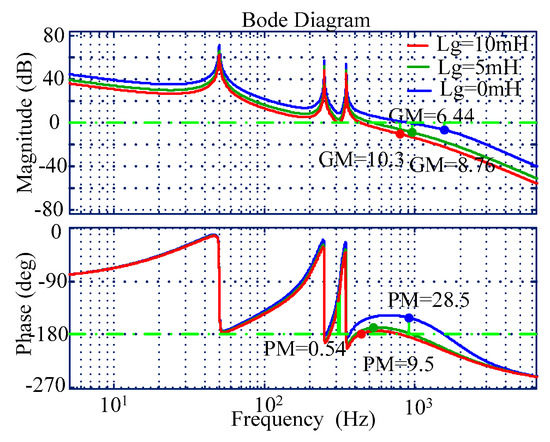
Figure 4.
Open-loop transfer function Bode diagram using the approach of harmonic controller.
From Figure 3 and Figure 4, no matter which control method is adopted in Scheme 1. As the grid impedance changes (Lg = 0 mH to Lg = 10 mH), the phase margin and cut-off frequency of the open-loop transfer function drop sharply. In addition, this could result in the slower dynamic response of the system, then poor stability, ultimately making it unstable. Therefore, Scheme 1 cannot adapt to the change in grid impedance, thus Scheme 2 is proposed to solve this problem.
3. Normalized Active Damping Voltage Feed-forward (Scheme 2)
It can be seen from previous study that if the grid current inner-loop produces the same virtual impedance effect as the capacitor current inner-loop, it is needed that both of their open-loop transfer functions are consistent around the natural resonant frequency [6,7]. Therefore, the feedback function of grid current inner-loop can be introduced as:
Figure 5 is a closed-loop block diagram of single-phase grid-connected inverter. The figure is composed of two parts, the main circuit and the control circuit. In order to analyze the worst case, pure inductance is selected as the grid impedance. Hc(s) is the feedback coefficient of capacitive current inner-loop; Hg(s) is the feedback function of grid current inner-loop; Gc(s) is the control compensator of grid current outer-loop; and Gfd(s) is the feed-forward coefficient.
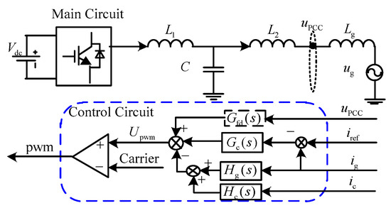
Figure 5.
Closed loop system of grid-connected inverter with Scheme 2.
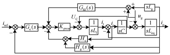
Figure 6.
System equivalent block diagram of Scheme 2.
Compared with Scheme 1, Scheme 2 introduces two new functions: Hg(s) and Gfd(s). According to the previous analysis, both a harmonic controller and PCC point voltage feed-forward are used to suppress the grid background harmonics. At the same time, both of them can change the cut-off frequency of open-loop transfer function , but their degree of change is different. The harmonic controller enlarges the proportional coefficient Kp of controller Gc(s), and feed-forward reduces the impact of grid impedance on the system. Therefore, when the system contains a harmonic controller, the PCC point voltage feed-forward is no longer used to suppress the grid background harmonics. It cooperates with the harmonic controller to change the cut-off frequency of the open loop and suppress the start-up inrush current. Therefore, the function of Gfd(s) represents the introduction of fundamental grid voltage and k(k ≤ 1) times harmonic voltage. The fundamental grid voltage feed-forward does not affect the cut-off frequency ωc of the open-loop transfer function ; it only improves the initial response speed of the system. The k times harmonic voltage feed-forward can change the open-loop cut-off frequency and restrain the grid background harmonic.
As before, in order to design parameters rapidly, the above controller is simplified to PI controller. Without considering the steady-state error around the fundamental frequency, the open-loop transfer function can be approximately divided into two parts according to the time constant T in the feedback function Hg(s) of the grid current loop [20,21].
The purpose of introducing the grid current inner-loop feedback is to increase the damping of the system. It is found from Formula (4) that the normalized damping can be added only when sT > 1. Therefore, the cut-off frequency crossing point should be in the part of sT < 1 in Formula (4) and the natural resonance frequency should be in the part of sT > 1 in Formula (4).
where
Therefore, at the frequency ω1res, the system should run on the part of sT > 1 in Formula (4). The time constant T of Hg(s) is used to convert to the part of sT > 1 in Formula (4), so the time constant of Hg(s) satisfies:
On the premise of satisfying Formula (5), the approximate open-loop transfer function expression and damping coefficient at cut-off frequency ωc, the amplitude and damping coefficient of the open-loop transfer function at harmonic frequency are obtained.
4. Parameter Design
4.1. Design of Control Parameters at Cut-off Frequency
According to the above analysis, the open-loop transfer function expression at cut-off frequency ωc is shown in Formula (6).
Formula (6) shows that the ωc decreases with the increase in grid impedance, and ωc is positively correlated with Kp, k, and Kg. This verifies the conclusion mentioned above that both the harmonic controller and the feed-forward control can increase the cut-off frequency ωc. In order to ensure that the cut-off frequency is within the range of [400,1000], Formula (7) can be obtained from Formula (6)
from Formula (7):
On the premise of satisfying Formula (8), then study Kp to make it satisfy Formula (7). Formula (8) shows that k > 0.1 and the larger the value of k, then the larger the value of Kg. Therefore, Formulas (7) and (8) show that k not only directly affects the cut-off frequency, but also indirectly changes the cut-off frequency through Kg. Therefore, under the premise of ensuring that the cut off frequency is within the range of 400 to 1000, the larger value of k will make the ωc larger, which means the larger bandwidth can be obtained.
It can be known from the part of sT < 1 in Formula (4) that the phase margin at the cut-off frequency ωc is related not only to the damping coefficient ξc but also to the ratio of the first natural resonance frequency ω1res corresponding to the cut-off frequency. For the convenience of analysis, the part of sT < 1 in Formula (4) can be changed to:
where
From Formula (9), it can be concluded that the open-loop transfer function consists of three parts: proportion, integral and second-order damping function. The integral part causes a phase lag of 90°, and the second-order damping function generates a phase lag of 90° at the natural resonance frequency . If the frequency-band damping before natural resonance frequency is larger, the phase lag will be more serious.
For the convenience of the following analysis, we needed to obtain the law of the natural resonance frequency of the part of sT < 1 in Formula (4) and the grid impedance. To start with, the assumption is that of the part of Ts < 1 in Formula (4) decreases with the increase in the grid impedance. So
where
Compared with Equation (8), when k is less than 1, it can be obtained as
Therefore, it can be obtained that the natural resonance frequency ω1res of the part of Ts < 1 in Formula (4) decreases with the increase in the grid impedance Lg. Therefore, when Lg = 10 mH, ω1res gets the minimum value, which can be known from Formula (5):
From Equation (9), the damping coefficient at cut-off frequency can be obtained as
It is known that ω1res decreases with the increase in Lg, while ω1resξc does not change. Therefore, the damping ξc increases with the increase in Lg and is positively correlated with Kg, k and Hc. That means the magnitude of ξc is related to these three parameters, and the growth ratio is only related to Kg and k, which can be known from Equation (14).
The ξc0 in Formula (14) is the value of ξc at Lg = 0. Therefore, it is necessary to lower the cut-off frequency to thereby increase the phase margin correspondingly, which is contradictory to maintaining a high bandwidth. In order to measure the change law of the relationship between cut-off frequency, damping coefficient and resonance frequency, a standardized proportional product function is introduced as:
In Formula (15), ωc0f, ξc0f and ω1res0f are the ratios of their real values to their initial values respectively. The smaller the value of function (15), the larger the phase margin at the cut-off frequency, but the lower the cut-off frequency. Therefore, a compromise between response speed and stability is needed. The value of is positively correlated with k and negatively correlated with Kg in Formula (15).
4.2. Design of Control Parameters at Resonant Frequency
The part of sT > 1 in Formula (4) can be simplified as
where
From Formula (16), it can be concluded that the open-loop transfer function consists of three parts: proportion, integral and second-order damping function. The natural resonance frequency ω2res obviously decreases with the increase in Lg, and the smaller the value of k, the slower the decrease tendency of ω2res. At this point, the damping part is divided into two parts. (ξ1res + ξ2res = ξres):
Formula (17) shows that the damping coefficient ξ1res varies with Lg. Moreover, as the k becomes smaller, the increase rate of ξ1res becomes slower, which is irrelevant to the operating frequency point, and it decreases compared with ξc of Formula (13). In addition, Formula (18) shows that the ξ2res is related to the operating frequency point.
The damping at resonance frequency is composed of Formula (17) and Formula (18). If the damping coefficient ξres is greater than 1, the second-order damping part will be divided into two first-order time constants. Due to the larger time constants affecting the phase margin at cut-off frequency ωc, the damping coefficient ξres should be less than 1. As the damping coefficient ξ1res increases with the increase in Lg, it is necessary to reduce or increase the damping coefficient ξ2res with the increase in Lg, but to ensure that the total damping coefficient is between 0.4 and 0.7.
In order to analyze the influence of the damping coefficient at the resonance frequency on the phase margin at the cut-off frequency with the change in Lg, a standardized proportional function (19) is introduced.
In Formula (19), ξ2ref0f and ω2res0f are the ratios of their real values to their initial values respectively.
When ξ2res decreases as the grid impedance Lg increases, the parameter design can be simplified, and the conditional Formula (20) needed to be satisfied is:
The ξ2ref0 in Formula (20) is the value of ξ2res at Lg = 0. The ratio of Formula (20) varies with grid impedance Lg and k, then a three-dimensional Figure 7 can be obtained.

Figure 7.
Function values of Formula (20) with different k and Lg.
It can be seen from the Figure 7 that when k < 0.5, the greater the grid impedance, the easier it is to satisfy Formula (20); however, when 0.5 < k < 1, the greater the grid impedance, the more difficult it is to meet the conditions. In addition, the previous analysis tries to keep sum of the two dampings unchanged. The smaller the k, the slower the ξ1res increase and the faster the ξ2res decrease, so it is not easy to find the value of k that meets the requirements intuitively. Therefore, it is necessary to further analyze the change ratio of the two dampings. Therefore, a standardized damping proportional function is given as
The ξ1ref0 in Formula (20) is the value of ξ1res at Lg = 0. From Equation (21), a three-dimensional graph of the relationship between the standardized value of the damping proportional function and the grid impedance Lg and feed-forward k can be obtained:
From Figure 8, it can be seen that when k ≤ 0.5, the standardized value of the damping ratio function does not change much with the increase in the grid impedance, but when k > 0.5, the standardized value of the damping ratio function increases with the increase in the grid impedance and increases rapidly. It is basically consistent with the conclusion shown in Figure 7. In Figure 8, when k ≤ 0.5, the function value increases first and then decreases with the increase in grid impedance Lg. Therefore, we can use the maximum product criterion to set two dampings as equal when the ratio is maximum, and then make the sum of the two dampings equal to the sum of the two dampings when Lg = 0 mH.
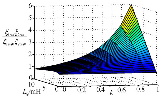
Figure 8.
Function values of Formula (21) with different k and Lg.
In Formula (15), when KgKpwm is taken as a constant value, the changing law of function value and the requirement for k value are basically consistent with that in Formula (21). When the range of k value is changed, considering the k value of Formula (21) from the viewpoint of mathematical calculation, it can generally satisfy Formula (15). Through the cut-off frequency Formulas (7) and (8) of the system, it can be known that the feed-forward coefficient k is expected to obtain a larger value to obtain a larger bandwidth. When considering the stability of the system, k needs to satisfy Formulas (15) and (21), so k = 0.5. At this point, Figure 8 becomes:
According to Figure 9, it can be found that when Lg = 6 mH, the normalized damping proportional function of Equation (21) reaches the maximum value, but when Lg > 6mH, the decrease tendency of function value is slower, which indicates that the sum of the final value of damping is larger than the sum of the initial value of damping. Therefore, by choosing , Lg = 6 mH can be brought into Equations (17) and (18), respectively.
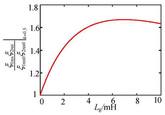
Figure 9.
Function values of Formula (21) varying with Lg when k = 0.5.
The parameters can get: Hc = 0.41; T = 10.8Kg. It can be seen that the added damping coefficient of grid current feedback mainly provides damping at the resonance frequency, restrains the resonance peak, and has little influence on the damping coefficient at the cut-off frequency. Thus, the damping coefficients at cut-off frequency and resonance frequency can be designed separately to meet the requirements of the phase margin and amplitude margin. At the same time, the magnitude of additional damping provided by the grid current inner-loop is related to the ratio of T to Kg.
Taking Hc = 0.041 and T = 10.8Kg into Equations (17) and (18), and summing up the two dampings, the total damping curve changing with the grid impedance is obtained in Figure 10 (red line):
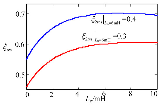
Figure 10.
ξres with impedance changes of Formula (13).
It can be seen from Figure 10 that the damping at the resonance frequency increases with grid impedance increasing. It is consistent with the conclusion shown in Figure 9. However, when Lg = 0 mH, the damping is small and the resonance peak easily occurs. It is found from Formulas (13) and (17) that ξ1res is directly related to ξc. For ξc, the smaller the ξc, the better. At the same time, ξ2res is not related to ξc, so . At this point, T = 8.13kad, a new damping curve is obtained in Figure 10 (blue line). Although the larger the damping of , the smaller the peak value at the resonance frequency, it has been found that the excessive damping at this point will also affect the phase margin at the cut-off frequency.
In order to get the parameter Kg, k = 0.5 can be taken into Equation (8), and we can get: Kg < 0.67 × 10⁻⁵.
The influence of Kg and Lg on the damping coefficient ξc can be obtained by introducing k = 0.5 and Hc = 0.41 into Equation (13):
It can be seen from Figure 11 that when Kg is constant, the damping coefficient increases with grid impedance. At the same time, when Kg becomes larger, the increasing extent of the damping coefficient is small. As the magnitude of the damping coefficient cannot fully represent the phase margin, so it needs to be judged by Formula (15). Therefore, the effect of Kg and Lg on the normalized value of the proportional product function is obtained by taking k = 0.5 into Equation (15) as shown in Figure 12.
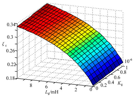
Figure 11.
Function value of Formula (13) with different Lg and Kg.
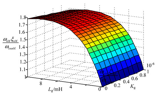
Figure 12.
Function value of Formula (15) with different Lg and Kg.
From Figure 12, it is found that the larger the Kg, the smaller the ratio of functions, which is consistent with the conclusion of Formula (15). Therefore, Kg is expected to obtain a larger value. In addition, it is necessary to analyze the influence of the damping coefficient at resonance frequency on the phase margin with the change of impedance Lg and Kg. Take k = 0.5, Hc = 0.41, T = 8.13Kg into Equation (19) and get Figure 13.
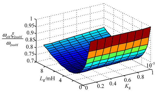
Figure 13.
Function value of Formula (19) with different Lg and Kg.
As can be seen from Figure 13, no matter what the grid impedance is, that the effect of Kg on the value of the function is negligible. When Lg = 4 mH, the parameters at the resonant frequency have the least influence on the phase margin. The parameter design of this paper is based on Lg = 6 mH, so it is necessary to verify the phase margin on the Bode diagram when Lg = 0, 4, 6, and 10 mH.
In the frequency band of the part of sT > 1 in Formula (4), the focus of the open-loop transfer function is the peak value around the resonance frequency, and the peak value at the natural resonance frequency is used to replace the amplitude margin. Therefore, the amplitude at the resonant frequency needs to satisfy Equation (23):
As the denominator of Formula (23) increases, the worst case is that when Lg = 0 mH, Kp < 0.09 is obtained. So far, the maximum meeting the requirements can be selected: Kg = 0.67 × 10⁻⁵, and bring it in Formula (7) to get 0.044 < Kp < 0.052. The larger the Kp is, the larger the cut-off frequency is. Therefore, Kp = 0.052 is chosen, and this satisfies Formula (12).
The above parameters neglect the influence of the phase lag of the PI controller, so the smaller Kr is, the smaller the influence on the system is. Generally, the inflection frequency of PI controller whose cut-off frequency is more than 5 times can be taken. The larger Kr is, the smaller the steady-state error is, so the Kr is 32.7.
By substituting the above parameters into Equations (15) and (18), the influence on the phase margin of the open-loop transfer function can be obtained. At the same time, because ω2res > ω1res, the influence of the two parts on the phase margin is different. In order to normalize, proportional factor should be introduced as
The curve with grid impedance changing is obtained according to (24).
It can be seen from Figure 14 that with the increase in grid impedance, the system parameters make the phase margin GM decreases first and then increases, but the overall change ratio is not large.
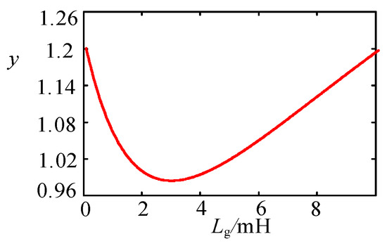
Figure 14.
y with grid impedance variation.
5. Analysis and Verification
5.1. Analysis of Control Parameters
The parameter design is mainly based on the phase margin PM, amplitude margin GM and cut-off frequency ωc of the open-loop transfer function T(s), so as to ensure the stability of the system. Through the above analysis, the control parameters under PI control are shown in Table 1.

Table 1.
Control parameters under PI controller.
The Bode diagram of the open-loop transfer function can be obtained by taking the parameters in Table 1 into Formula (3), as shown in the Figure 15.
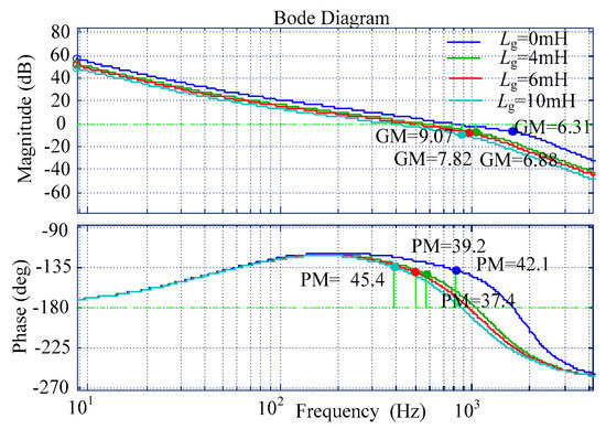
Figure 15.
Bode diagram of open loop transfer function with different Lg.
It is found that the amplitude margin increases with grid impedance Lg increasing. The amplitude margin is related to the amplitude at the second resonance frequency. The larger the damping at the resonance frequency is, the smaller the resonance amplitude is. This is consistent with the conclusion shown in Figure 10 that the damping at the resonance frequency increases with the increase in the Lg. The phase margin decreases first and then increases with the increase in Lg. The phase margin is related to the parameters at the cut-off frequency, which is completely consistent with the conclusion shown in Figure 14.
As mentioned above, compared with the harmonic controller and PI controller, the amplitude curve of the open-loop transfer function under the harmonic controller moves up under the same proportional coefficient. Therefore, Khp = 0.035 is obtained by the Bode diagram. The Bode diagram of the open-loop transfer function can be obtained by introducing this parameter into Formula (3).
It can be seen from the diagram that the phase margin and amplitude margin of the open-loop transfer function do not change much with the increase in the Lg, and can adapt to the change in equivalent impedance of power grid well, and are within acceptable range compared with the parameters of PI controller.
According to Figure 3, Figure 4 and Figure 16, with the increase in grid impedance (Lg = 0 mH to 10 mH), for the traditional strategy, the phase margin drops sharply; this could result in the slower dynamic response of the system, then poor stability and ultimately making it unstable; for the normalized active damping strategy, the phase margin is basically unchanged.
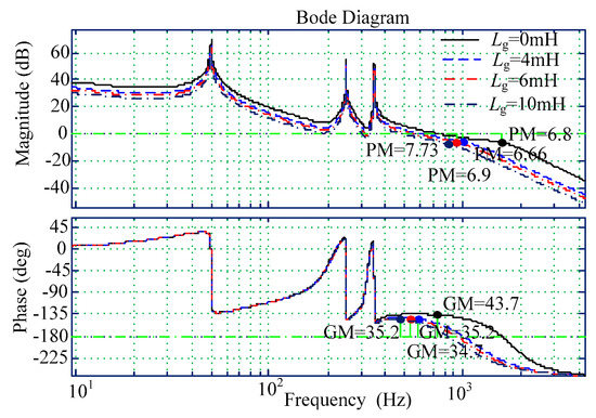
Figure 16.
Open loop transfer function T(s) bode diagram of Scheme 2.
5.2. Simulation Analysis
In order to simulate the grid background harmonic, the grid background harmonic, as shown in Table 2, is added to the grid voltage.
Table 2.
The parameters of the grid background harmonics.
Figure 17 shows the grid voltage waveform with harmonics.
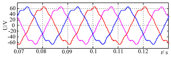
Figure 17.
Grid voltage waveform with harmonics.
In the case of the strong grid, the two cases in Scheme 1 are compared with the normalized active damping scheme proposed in this paper, the inverter is in a stable state, and the simulation of the Scheme 1 under the strong grid is no longer necessary to analyzed. Figure 18 and Figure 19 are the simulation waveforms of the grid current under Scheme 1 when the grid impedance is Lg = 5 mH.
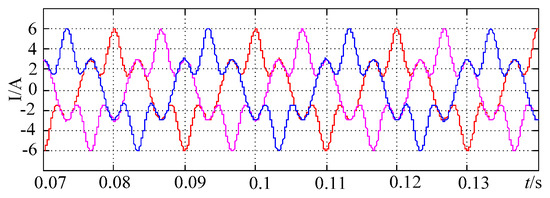
Figure 18.
Waveform of the grid current using the feed-forward control when Lg = 5 mH in Scheme 1.
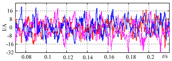
Figure 19.
Waveform of the grid current using harmonic quasi proportional integral resonance controller (H-QPIR) control when Lg = 5 mH in Scheme 1.
Figure 18 shows that the system is stable, but the ability to suppress harmonics is limited. The grid current contains a large number of fifth and seventh harmonics, which is consistent with the Bode diagram in Figure 3. The open-loop gain in the low frequency band is low and the ability to suppress harmonics is poor; Figure 19 shows that the system is in an unstable state, and the harmonics around the cut-off frequency are amplified, which is consistent with the Bode diagram in Figure 4. The harmonic amplification is caused by the low phase margin.
Figure 16 in Scheme 2 shows that the phase margin and cut-off frequency of the open-loop transfer function T(s) are similar when Lg = 4 and 6 mH, then Lg = 5 mH is used in simulation.
Figure 20, Figure 21 and Figure 22 verify the Bode diagram of T(s) of Figure 16. It shows that the system can maintain stability when the equivalent impedance of the power grid changes from 0 to 10 mH and can suppress the grid background harmonics. The only difference is that the dynamic response becomes slower with the increase in the Lg. The given current amplitude increases abruptly from 3 to 5 A at 0.093 s, as shown in Figure 20, Figure 21 and Figure 22. When the grid inductance Lg = 0 mH, the dynamic rise time of the incoming current is 0.002 s; when the grid inductance Lg = 5 mH, the rise time of the grid current is 0.003 s; when the grid inductance Lg = 10 mH, the rise time of the grid current is 0.005 s. The bigger the grid impedance, the slower the transient response of the grid current and the PCC point voltage is, which is consistent with the conclusion in Figure 16.
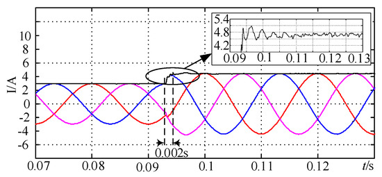
Figure 20.
Grid current waveform of the Scheme 2 when Lg = 0 mH.
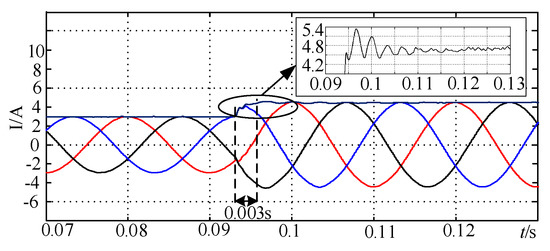
Figure 21.
Grid current waveform of the Scheme 2 when Lg = 5 mH.
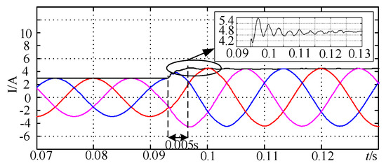
Figure 22.
Grid current waveform of the Scheme 2 when Lg = 10 mH.
According to the previous analysis, both the traditional active damping strategy and the normalized active damping strategy are in stable state under strong grid. When the grid impedance is 5 mh, according to Figure 18, Figure 19 and Figure 21, the previous strategy has poor ability to suppress harmonics, while the normalized active damping strategy has strong ability to suppress harmonics. In addition, the previous strategy cannot adapt to the changing grid impedance, and the normalized active damping strategy can still ensure the stable operation of the system when the grid impedance changes from 0 to 10 mH.
5.3. Experimental Verification
In order to verify the correctness of the above theoretical analysis and simulation, a three-phase grid-connected inverter experimental platform of DSP (Digital Signal Processor) + FPGA (Field Programmable Gate Array) control board was built in the laboratory. Figure 23 shows the experimental platform. DSP adopts TMS320F28335 of TI company (Dallas, TX, USA), FPGA adopts EP3C25Q240C8N of Altera company (San Jose, CA, USA). The parameters used in experiments are as follows: Vdc = 80 kV, f1 = 50 Hz, fs = 20 KHz, ug = 50 V. The other system parameters are shown in Table 1.
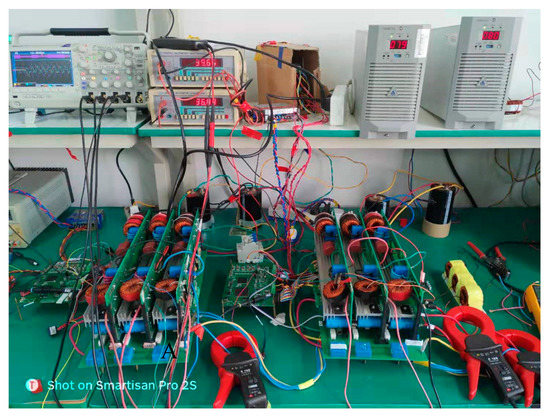
Figure 23.
Experimental platform.
Figure 24 is the voltage waveform with grid background harmonics; Figure 25 is the experimental waveform corresponding to Figure 18; Figure 26 is the experimental waveform corresponding to Figure 19; Figure 27, Figure 28 and Figure 29 show the experimental waveform of Figure 20, Figure 21 and Figure 22. The four curves in the figure represent three-phase current and d-axis current after equivalent coordinate transformation.
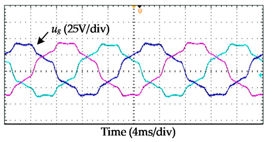
Figure 24.
Experimental waveform of grid voltage with grid background harmonic.
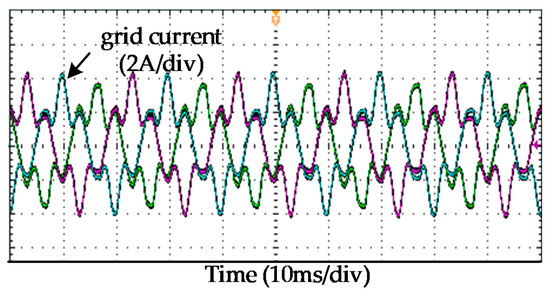
Figure 25.
Experimental waveforms of the grid current using feed-forward control in Scheme 2 when Lg = 5 mH
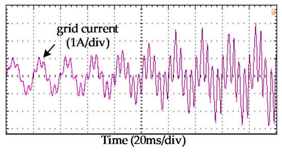
Figure 26.
Experimental waveforms of grid current using H-QPIR in Scheme 1 when Lg = 5 mH.
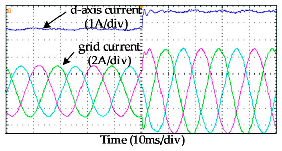
Figure 27.
Experimental waveforms of grid current in Scheme 2 when Lg = 0 mH.
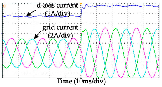
Figure 28.
Experimental waveforms of grid current in Scheme 2 when Lg = 5 mH.
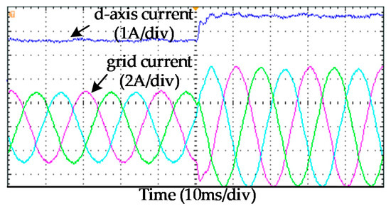
Figure 29.
Experimental waveforms of grid current in Scheme 2 when Lg = 10 mH.
The grid current in Figure 25 contains a lot of harmonics, which is consistent with the simulation waveform in Figure 18. In Figure 26, the grid current loses stability, which is consistent with the simulation waveform in Figure 19. Figure 27, Figure 28 and Figure 29 show that with the increase in the grid impedance, the grid background harmonics can be well suppressed, which is consistent with the simulation waveform in Figure 20, Figure 21 and Figure 22. In Figure 30 and Figure 31, compared with Scheme 1, Scheme 2 has more advantages in harmonic suppression in a weak grid.
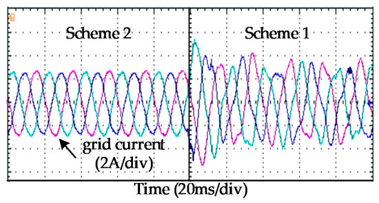
Figure 30.
Experimental waveforms of grid current in different schemes when Lg = 3 mH.
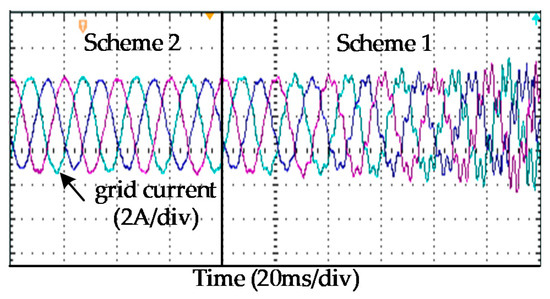
Figure 31.
Experimental waveforms of grid current in different schemes when Lg = 6 mH.
When the grid impedance is 5 mH, according to Figure 25, Figure 26 and Figure 28, the previous strategy has poor ability to suppress harmonics, while the novel strategy mentioned in this paper has a strong ability to suppress harmonics. According to Figure 30 and Figure 31, it can be intuitively found that the capacitor current feedback active damping cannot adapt to the change in grid impedance. Moreover, the normalized active damping solves the problem of the traditional strategy, the system can operate stably when the grid impedance varying between 0 and 10 mH.
The experimental results show that the traditional control strategies can also suppress harmonics, but the ability is limited in weak grids. The normalized active damping strategy can suitable for wide-range grid impedance variation and ensure the stability of grid connected system.
6. Conclusions
In view of the disadvantage in that the LCL grid-connected inverters with traditional control schemes cannot adapt to the change in the equivalent impedance of a power grid, three new control variables are introduced, and the normalized active damping strategy is designed through detailed theoretical deduction. By optimizing the parameters, the changing tendency of the damping coefficient of the grid-current inner loop is opposite to that of capacitor current inner-loop. Then, the grid-connected inverters can maintain stability when the equivalent impedance of the power grid changes from 0 to 10 mH and can suppress the grid background harmonics. The sum of the damping produced by these two damping is basically unchanged with the change of grid impedance. The derivation process of the theoretical basis of this method is slightly complicated, but only a few formulas are needed to complete the parameter design in practical application. For different LCL filter parameters, according to the design steps in this paper, the corresponding control parameters can be obtained, and the following conclusions can be drawn.
(1) The active damping generated by capacitive current loop is positively correlated with the equivalent impedance of the power grid. When the damping system becomes larger, the LCL filter will become the cascade connection of an integrator and two first-order inertia links, which will reduce the phase margin of the open-loop transfer function.
(2) In this paper, the functional relationship between cut-off frequency ωc, damping coefficient ξ and natural resonance frequency ωres related to phase margin is introduced, which is suitable for judging the phase margin of all second-order functions and can be used to observe the variation of the phase margin.
(3) The sum of the damping produced by capacitive current loop and grid current loop is basically unchanged with the change of grid impedance. It is suitable for the system of wide-range grid impedance variation, and has strong robustness.
(4) Proportional feed-forward of grid voltage is not only used for harmonic suppression, but also positively correlated with the cut-off frequency ωc of the open-loop transfer function of the system, and thus it can be used to improve the cut-off frequency.
Author Contributions
Conceptualization, Y.L. and X.W.; methodology, Y.L., Q.Y. and X.W.; formal analysis, Y.L.; validation, Y.L. and Q.Y.; writing—original draft, Y.L.; writing—review and editing, Y.L., X.W. and X.Z.; supervision, X.W. and C.Z. All authors have read and agreed to the published version of the manuscript.
Funding
This research was funded by National Natural Science Foundation of China, grant number 51607154 and Foundation of the Higher Education Institutions of Hebei Province, grant number QN2017362. Project Supported by the Natural Science Foundation of Hebei Province, China, grant number E2018203152.
Conflicts of Interest
The authors declare no conflict of interest.
References
- Blaabjerg, F.; Teodorescu, R.; Liserre, M.; Timbus, A.V. Overview of Control and Grid Synchronization for Distributed Power Generation Systems. IEEE Trans. Ind. Electron. 2006, 53, 1398–1409. [Google Scholar] [CrossRef]
- Gullvik, W.; Norum, L.; Nilsen, R. Active damping of resonance oscillations in LCL-filters based on virtual flux and virtual resistor. In Proceedings of the European Conference on Power Electronics, Aalborg, Denmark, 2–5 September 2007; pp. 1–10. [Google Scholar]
- Malinowski, M.; Bernet, S. A simple voltage sensorless active damping scheme for three-phase PWM converters with an LCL filter. IEEE Trans. Ind. Electron. 2008, 55, 1876–1880. [Google Scholar]
- Dannehl, J.; Liserre, M.; Fuchs, F.W. Filter-Based Active Damping of Voltage Source Converters with LCL Filter. IEEE Trans. Ind. Electron. 2011, 58, 3623–3633. [Google Scholar] [CrossRef]
- Yao, W.; Yang, Y.; Zhang, X.; Blaabjerg, F.; Loh, P.C. Design and Analysis of Robust Active Damping for LCL Filters Using Digital Notch Filters. IEEE Trans. Power Electron. 2016, 32, 2360–2375. [Google Scholar] [CrossRef]
- Pan, D.; Ruan, X.; Bao, C.; Li, W.; Wang, X. Capacitor-Current-Feedback Active Damping With Reduced Computation Delay for Improving Robustness of LCL-Type Grid-Connected Inverter. IEEE Trans. Power Electron. 2014, 29, 3414–3427. [Google Scholar] [CrossRef]
- Sun, J.; Wang, Y.; Gong, J.; Zha, X.; Li, S. Adaptability of weighted average current control to the weak grid considering the effect of grid-voltage feedforward. In Proceedings of the 2017 IEEE Applied Power Electronics Conference and Exposition (APEC), Tampa, FL, USA, 26–30 March 2017; pp. 3530–3535. [Google Scholar]
- Shen, G.; Xu, D.; Cao, L.; Zhu, X. An Improved Control Strategy for Grid-Connected Voltage Source Inverters With an LCL Filter. IEEE Trans. Power Electron. 2008, 23, 1899–1906. [Google Scholar] [CrossRef]
- Xu, J.; Xi, S. LCL-resonance damping strategies for grid-connected inverters with LCL filters: A comprehensive review. J. Mod. Power Syst. Clean Energy 2018, 6, 292–305. [Google Scholar] [CrossRef]
- He, J.; Li, Y.W. Generalized Closed-Loop Control Schemes with Embedded Virtual Impedances for Voltage Source Converters with LC or LCL Filters. IEEE Trans. Power Electron. 2012, 27, 1850–1861. [Google Scholar] [CrossRef]
- Tang, Y.; Loh, P.C.; Wang, P.; Choo, F.H.; Gao, F. Exploring Inherent Damping Characteristic of LCL-Filters for Three-Phase Grid-Connected Voltage Source Inverters. IEEE Trans. Power Electron. 2012, 27, 1433–1443. [Google Scholar] [CrossRef]
- Yang, D.; Ruan, X.; Wu, H. Impedance Shaping of the Grid-Connected Inverter with LCL Filter to Improve Its Adaptability to the Weak Grid Condition. IEEE Trans. Power Electron. 2014, 29, 5795–5805. [Google Scholar] [CrossRef]
- Zheng, C.; Zhou, L.; Yu, X.; Li, B.; Liu, J. Online phase margin compensation strategy for a grid-tied inverter to improve its robustness to grid impedance variation. IET Power Electron. 2016, 9, 611–620. [Google Scholar] [CrossRef]
- Peña-Alzola, R.; Liserre, M.; Blaabjerg, F.; Sebastián, R.; Dannehl, J.; Fuchs, F.W. Systematic Design of the Lead-Lag Network Method for Active Damping in LCL-Filter Based Three Phase Converters. IEEE Trans. Ind. Inform. 2013, 10, 43–52. [Google Scholar] [CrossRef]
- Yang, S.; Lei, Q.; Peng, F.Z.; Qian, Z. A Robust Control Scheme for Grid-Connected Voltage-Source Inverters. IEEE Trans. Ind. Electron. 2010, 58, 202–212. [Google Scholar] [CrossRef]
- Kahrobaeian, A.; Mohamed, A.R.I. Robust Single-Loop Direct Current Control of LCL-Filtered Converter-Based DG Units in Grid-Connected and Autonomous Microgrid Modes. IEEE Trans. Power Electron. 2014, 29, 5605–5619. [Google Scholar] [CrossRef]
- Xu, J.; Xie, S.; Huang, L.; Ji, L. Design of LCL-filter considering the control impact for grid-connected inverter with one current feedback only. IET Power Electron. 2017, 10, 1324–1332. [Google Scholar] [CrossRef]
- Pérez, J.; Cóbreces, S.; Wang, X.; Blaabjerg, F.; Griñó, R. A robust grid current controller with grid harmonic and filter resonance damping capabilities using a closed-loop admittance shaping. In Proceedings of the 2017 IEEE Applied Power Electronics Conference and Exposition (APEC), Tampa, FL, USA, 26–30 March 2017; pp. 2625–2632. [Google Scholar]
- Pérez, J.; Cobreces, S.; Grino, R.; Sánchez, F.J. H∞ current controller for input admittance shaping of VSC-based grid applications. IEEE Trans. Power Electron. 2016, 32, 3180–3191. [Google Scholar] [CrossRef]
- Huang, J.; Yuan, X. Impact of the voltage feed-forward and current decoupling on VSC current control stability in weak grid based on complex variables. In Proceedings of the 2015 IEEE Energy Conversion Congress and Exposition (ECCE), Montreal, QC, Canada, 20–24 September 2015; pp. 6845–6852. [Google Scholar]
- Xu, J.; Xie, S.; Tang, T. Active Damping-Based Control for Grid-Connected LCL -Filtered Inverter with Injected Grid Current Feedback Only. IEEE Trans. Ind. Electron. 2014, 61, 4746–4758. [Google Scholar] [CrossRef]
- Xu, J.; Xie, S.; Zhang, B.; Qian, Q. Robust Grid Current Control with Impedance-Phase Shaping for LCL-Filtered Inverters in Weak and Distorted Grid. IEEE Trans. Power Electron. 2018, 33, 10240–10250. [Google Scholar] [CrossRef]
- Wang, X.; Blaabjerg, F.; Loh, P.C. Grid-Current-Feedback Active Damping for LCL Resonance in Grid-Connected Voltage-Source Converters. IEEE Trans. Power Electron. 2015, 31, 213–223. [Google Scholar] [CrossRef]
- Wang, X.; Ruan, X.; Liu, S.; Chi, K.T. Full Feedforward of Grid Voltage for Grid-Connected Inverter With LCL Filter to Suppress Current Distortion Due to Grid Voltage Harmonics. IEEE Trans. Power Electron. 2011, 25, 3119–3127. [Google Scholar] [CrossRef]
- Li, W.; Ruan, X.; Pan, D.; Wang, X. Full-Feedforward Schemes of Grid Voltages for a Three-Phase, LCL-Type Grid-Connected Inverter. IEEE Trans. Ind. Electron. 2013, 60, 2237–2250. [Google Scholar] [CrossRef]
- Wang, X.; Yang, Q.; Qing, H.; Zhang, C. Hybrid Active Damping Control Method for Grid Connected LCL Inverters under Weak Grid. In Proceedings of the 2018 IEEE International Power Electronics and Application Conference and Exposition (PEAC), Shenzhen, China, 4–7 November 2018; pp. 1–6. [Google Scholar]
- Seo, S.; Cho, Y.; Lee, K.B. LCL Filter Design for Grid Connected Three-Phase Inverter. In Proceedings of the 2018 2nd International Symposium on Multidisciplinary Studies and Innovative Technologies (ISMSIT), Ankara, Turkey, 19–21 October 2018; pp. 1–4. [Google Scholar]


© 2020 by the authors. Licensee MDPI, Basel, Switzerland. This article is an open access article distributed under the terms and conditions of the Creative Commons Attribution (CC BY) license (http://creativecommons.org/licenses/by/4.0/).