Abstract
Recent advances in deep learning have shown exciting promise in various artificial intelligence vision tasks, such as image classification, image noise reduction, object detection, semantic segmentation, and more. The restoration of the image captured in an extremely dark environment is one of the subtasks in computer vision. Some of the latest progress in this field depends on sophisticated algorithms and massive image pairs taken in low-light and normal-light conditions. However, it is difficult to capture pictures of the same size and the same location under two different light level environments. We propose a method named NL2LL to collect the underexposure images and the corresponding normal exposure images by adjusting camera settings in the “normal” level of light during the daytime. The normal light of the daytime provides better conditions for taking high-quality image pairs quickly and accurately. Additionally, we describe the regularized denoising autoencoder is effective for restoring a low-light image. Due to high-quality training data, the proposed restoration algorithm achieves superior results for images taken in an extremely low-light environment (about 100× underexposure). Our algorithm surpasses most contrasted methods solely relying on a small amount of training data, 20 image pairs. The experiment also shows the model adapts to different brightness environments.
1. Introduction
Image restoration is a challenging task, particularly in an extremely dark environment. For example, the recovery of images captured in a scene where the light is very dark is a difficult problem. There are two ways to solve the problem: relying on hardware and relying on software. In the aspect of hardware, the adjustment of the camera settings can partially solve the problem, but there are still difficulties: (1) a higher sensitivity value of the image sensor increases brightness, but it also increases high sensitivity noise, and, although the ISO value in the latest cameras can be set to 25,600, the images with an ISO over 400 should have more noise; (2) the larger aperture receives more light, but it also leads to worse sharpness and a shallower depth of field; (3) extending exposure time is one of the most direct solutions, but a little movement should lead to blurred imaging under the condition; (4) the larger size of the photosensitive element receives more photons, although the size of the photosensitive element is limited by camera size and cost; (5) using flash helps to capture more light, however, the flash range is limited and flash is forbidden in some situations.
In addition to the suitable hardware settings, some sophisticated algorithms have been designed to restore the images in the dark. Many denoising, deblurring, color calibration, and enhancement algorithms [1,2,3,4,5] are applied to low-light images. These algorithms only deal with normal low-light images but are inefficient for the extremely low-light images with brightness as low as 1 lumen. An alternative method, burst alignment algorithms [6,7,8], uses multiple pictures taken continuously. However, this kind of method still loses efficacy on the pictures in extremely low-light conditions. Chen et al. [9] proposed a deep learning end-to-end method which can restore images with only 0.1 lumens. However, this method was trained with massive amounts of training data and needed a huge computational cost. It is well known the deep learning algorithms require big data. One of the reasons is that the quality of partial data is poor. By obtaining better training data, the algorithm can accomplish the same result with less data.
In the past, the low-light data were basically collected in the low-light environment, while the ground truth data were collected by long exposure. This collecting method had many difficulties and generated low-quality training data. We propose a new method to collect dark pictures and corresponding normal exposure pictures by adjusting camera settings in the daytime.
We use an end-to-end neural network to restore the extremely low-light image only by 20 high-quality image pairs based on the work of [9,10]. Our contributions in this paper are summarized as follows: (1) we propose a new low-cost method to capture high-quality image pairs, including dark pictures and corresponding normal exposure pictures; (2) we use the theory of the regularized denoising autoencoder to explain why the algorithm works effectively; (3) our proposed algorithm can restore images taken in an extremely dark environment (100× underexposure light level) by only using 20 image pairs.
The rest of this paper is organized as follows. Related work about low-light images restoration is proposed in Section 2. The image acquisition method and the framework of the neural network are shown in Section 3. The detailed experimental results are shown in Section 4. Several problems that require further research are put forward in Section 5. The paper concludes with Section 6.
2. Related Work
The restoration of low-light images has been extensively studied in the literature. In this section, we provide a short review of related work.
2.1. Low-Light Image Datasets
Well-known public image datasets, such as PASCAL VOC [11], ImageNet [12], and COCO [13] have played a significant role in traditional computer vision tasks. Because less than 2% of the images in these datasets were taken in a low-light environment, the public datasets were unsuitable for training low-light image restoration.
Many researchers proposed low-light image datasets. LLnet [14] darken the original images to simulate low-light images. The original images were used as a ground truth; the generated dark images were artificial. The authors of [5] proposed a new dataset of 3000 underexposed images, each with an expert-retouched reference. PolyU [15] collected real-world noisy images taken from 40 scenes, including indoor normal lighting, dark lighting, and outdoor normal-light scenes. However, the brightness of the images from these datasets is dusky, not extremely black. SID [9] proposed an extremely dark image dataset captured by Sony and Fuji cameras, including 5094 short exposure images and 424 long-exposure images. LOL [16] consists of 500 image pairs. The ExDARK [17] dataset is made up of images captured in real environments, containing various objects. Because the images need careful adjustment of the camera settings in dark conditions, the previously mentioned databases have two common problems: the high cost of collecting data and very few high-quality images.
2.2. Image Denoising
According noise is one of the significant obstacles in the restoration of low-light images; denoising is a notable subtask in low-light enhancement tasks. A classic traditional method of dealing with the low-light image is scaling luminosity and the followed denoising procedure. Image denoising is an often-traversed topic in low-level computer vision. Many approaches have been proposed, such as total variation [18], sparse coding [19], and 3D transform-domain filtering (BM3D) [20], etc. These approaches are grouped into traditional denoising methods. Their effectiveness is often based on an image prior’s information, such as smoothness, low rank, and self-similarity, etc. Unfortunately, most traditional methods only work more effectively for the synthetic noise data, such as salt pepper and Gaussian noise, but the performance of the methods sharply drops for noisy images taken in real-world environments.
Researchers have also widely explored the application of deep learning networks to image denoising. Important methods of deep learning include deep illumination estimation [5], end-to-end convolutional networks [9,21], autoencoders [22,23], and multi-layer perceptron [24]. Generally, most methods based on deep learning work better than traditional methods. However, the former has the requirement of huge amounts of training data.
Except for single image denoising, the alternative, multiple-image denoising [6,7,25], achieves better results since more information is collected. However, it is difficult to select the “lucky image” and the correspondence estimation between images. On some occasions, taking more than one image was infeasible.
2.3. Low-Light Image Restoration
One basic method is histogram equalization to expand the dynamic range of the images. The recent effort on low-light image restoration is the learning-based methods. For instance, the authors of [14] proposed a deep autoencoder approach. WESPE [26] proposed a weakly supervised image-to-image network based on a Generate Adversarial Network (GAN). However, WESPE was more focused on image enhancement. In addition, other methods include the approach based on dark channel prior [27], the wavelet transform [23], and illumination map estimation [28], etc. These methods mentioned above only deal with the images captured in a normal dark environment, such as dusk, morning, and shadow, etc. The end-to-end model proposed by Chen et al. [9] could restore extremely low-light images using RAW sensor data. However, its model was heavyweight. In sum, the current research suggests that either the image in the extreme dark cannot be restored or the algorithms require big data.
3. The Approach
3.1. The End-to-End Pipeline Based on Deep Learning
The pipelines based on deep learning and the traditional method can be used to restore low-light images. Two kinds of pipelines are shown in Figure 1. The deep learning model (the top sub-image) is an end-to-end method. This method generates a model from image pairs, while the traditional method cascades a sequence of low-level vision processing procedures, such as luminosity scaling, demosaicing, denoising, sharpening, and color correction, etc. In Figure 1, luminosity scaling and cBM3D are selected as the major procedures in the traditional method.
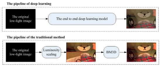
Figure 1.
The two categories of pipelines concerning low-light restoration. The top sub-image shows the pipeline based on deep learning. The bottom sub-image shows a traditional image processing pipeline. The toy images on the right side are the results of the two pipelines, respectively. The sub-image surrounded by a red line box is the zoom-in image. BM3D = 3D transform-domain filtering.
In the pipeline of the traditional method, the first step is luminosity scaling. The images taken by the camera Nikon D700 are Nikon Electric Film (NEF) RAW images with 14 bits. This means that the maximum brightness value is 214, that is, 16,384. Due to the image in the extremely dark condition, the brightness values of the pixels are distributed between 1 and 50. The procedure of light scaling can be expressed as a formula: vx/vmax × 16,384. The parameter vx in the formula represents the brightness value of a pixel, and vmax represents the max brightness value of all pixels. The simple luminosity scaling also amplifies the noise information in the images. The high noise is demoed in the zoom-in image surrounded by the red box after luminance scaling. The second step is noise reduction by BM3D.
In our work, the deep learning neuron network is proposed for direct single image restoration of extremely low-light images. Specifically, a convolutional neural network [29] U-net [10] is used for processing, inspired by the recent algorithms in the work of [9,10]. The structure of the network is shown in Figure 2, and the details about the structure are listed in Table 1.
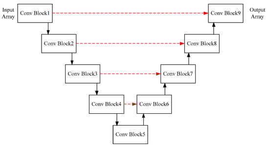
Figure 2.
The structure of the network. The input array is a 4D data converted from the original RAW image. Convolutional block is abbreviated as “Conv Block”, which represents a convolutional block including 2D convolutional layer and pooling layer. The red dotted arrow represents copy and crop operations.

Table 1.
The parameters of the neuronal network. The parameter “32 [3,3]” represents that the output array size is 32 and the convolutional kernel size is 3 × 3.
3.2. Regularized Denoising Autoencoder
In our study, we selected an autoencoder neural network [30,31] similar to U-net to restore dark images. The autoencoder is a neural networks that is trained to attempt to map the input to the output. In other words, it is restricted in some ways to learn the useful properties of the data. It has many layers internally called the hidden layer. The network is divided into two parts: an encoder function h = F(x) and a decoder function G(h) which generates the reconstruction.
Regularized technology [32,33] is used to solve the invalidation of the over-complete autoencoder. The case is called over-complete when the hidden dimension is greater than the input. The over-complete autoencoders fail to learn anything useful if the encoder and decoder have a large number of parameters. Regularized autoencoders use a loss function to learn useful information from the input. The useful information includes the sparsity of the representation, robustness to noise, and robustness to the missing input. In particular, the clear and real image data is useful information, hidden in the dark background. In one word, regularization enables the nonlinear and over-complete autoencoder to learn useful information about the data distribution.
The denoising autoencoder (DAE) [34,35] is one of the autoencoders with corrupted data as input and clear data as output by a trained model. The structure of a DAE is shown in Figure 3. It aims to learn a reconstruction distribution precontstruct(y|x) by the given training pairs (x,y). The DAE minimizes the function L(y,G(F(x))) to obtain the useful properties, where x is a corrupted data relative to the original data y. Specifically, in our study, data x indicates the images with dark noise and data y indicates the ground truth images.
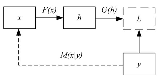
Figure 3.
The structure of a denoising autoencoder (DAE). The input data tagged as x and output data tagged as y represent the noisy data and ground truth, respectably. The function F(x) and G(h) represent the encoder and decoder. The map M(x|y) represents the procedure of generating x from y.
The first step is sampling y from the training data. The second step is sampling the corresponding data point x by M(x|y). The third step is estimating the reconstruction distribution by pdecoder(y|h) with h the output of encoder and pdecoder defined by the decoder G(h). DAE is a feedforward network and trained by the methods of any other feedforward network. We can perform gradient-based approximate minimization on the negative log-likelihood. For example, the stochastic gradient descent can be written by:
In Equation (1), the is the distribution calculated by the decoder and the is the training data distribution.
3.3. The Procedure of Collecting Data
The traditional low-light enhancement methods cascade the procedures: scaling, denoising, and color-correcting. The traditional methods do not need the ground truth images during processing. On the contrary, a deep learning neural network must train the data before the testing phase. The training and testing phases are shown in Figure 4. The upper part of this figure shows that the training data consists of two parts: the low-light (dark) images and corresponding normal-light images. Every image pair in the two parts has the same size and shooting range and aligns pixel by pixel. There are only a few low-light image datasets available, an example from one of these datasets is seen in the upper left. The learned-based model can learn the fitting parameters to map the image pairs. The mapping relationship from the low-light images to normal-light images is non-linear, and thus deep learning is appropriate.
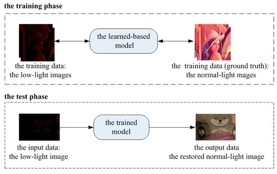
Figure 4.
The schematic diagram of the train and test phase in the deep learning approach. The upper sub-image shows the training phase. The bottom sub-image shows the test phase using the trained model generated in the training phase.
The bottom sub-image of Figure 4 shows the test phase. In the test phase, the low-light images are inputted into the trained model and the restored normal-light images are outputted. In addition, the output restored image (bottom right corner) is unknown, the other three kinds of images are known. Another significant point is that the training and the test images are independent.
In order to improve the effectiveness of the restoration, we can start from the two aspects of the algorithm and the training data. In this section, we describe the training data. Due to the large computational cost of the training data, data collection becomes an obstacle to the deep learning algorithms.
The data collecting method in other deep learning literature is shown as the upper sub-image of Figure 5. The low-light datasets based on deep learning in the computer vision community are almost collected in low-light conditions, shown as the left box of the upper of Figure 5. The corresponding ground truth images are also taken in low-light conditions, shown as the right box of the upper. For taking normal exposure images, the camera is set to a higher ISO, larger aperture, longer exposure time, larger light-sensing element, and flash. However, such settings reduce the quality of the images.
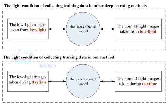
Figure 5.
The different light conditions during the phase of collecting training images in deep learning. The upper sub-figure shows that the image pairs both captured in low-light conditions. In the below sub-figure, our proposed image acquisition method captures images during the daytime. In our method, the low-light images are taken in the normal-light condition.
We collected the training data during the daytime, normal-light condition, shown as the button sub-image of Figure 5. We named the collecting method the NL2LL (normal-light to low-light). The environment with enough light brings convenience to shoot high-quality data. Three pillars of the photography: shutter speed, ISO, and aperture can be set as “better” parameters during the daytime. We set the shorter exposure speeds, lower ISO, and larger aperture values to take the dark images during the daytime.
The influence of the aperture is rarely discussed in the relevant literature. Aperture is defined as the opening in the lens through which light passes to enter the camera. Small aperture numbers represent a large aperture opening size, whereas large numbers represent small apertures. The critical effect of the aperture is the depth of field. Depth of field is the amount of the photograph that appears sharp from front to back. According to the principles of optics, a larger aperture size (smaller aperture value) leads to a shallower depth of field and therefore more defocus blur.
The effect of the aperture size on the image depth of field is shown in Figure 6. The left half of this figure has a “thin” depth of field, where the background is completely out of focus. On the contrary, the right sub-image of Figure 6 has a “deep” depth of field, where both the foreground and the background are sharp; the camera focuses on the foreground. Because the zoom-in images surrounded by the solid red box are near the focus point, both images (the first and the third image at the bottom) are clear. However, the distance between the dotted red region and the camera is far from that between the focus point and the camera. According to the principles of optics, the background area away from the focus point becomes blurred with a large aperture camera setting. The zoom-in sub-image taken in the big aperture size (the second image at the bottom) is more blurred than the respective sub-image taken in the small aperture size (the fourth image at the bottom).
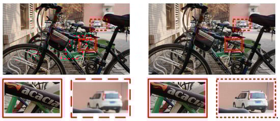
Figure 6.
The influence of the aperture size on the image quality. The aperture of the left and right images is set as 4 (large aperture size) and 25 (small aperture size), respectively. The center of the red circle is the location of the focal point. The area surrounded by the solid red box and dotted red box is in foreground and background, respectively.
If the images are taken in dark conditions, the aperture must be set as large as possible to receive more light. The large aperture setting in the camera inevitably results in a large amount of background blur. The training dataset used in deep learning has many image pairs. Every image pair consists of a low-light image and a corresponding normal-light image. To achieve high-quality data, each pixel pair in both images must match one-to-one. Unfortunately, the blur of some pixels impacted the quality of the training data [9,14].
The large aperture size should blur the image. It is also plain to see that the longer exposure time and the higher ISO reduces the quality of the image pair. More specifically, it is harder to align the two images pixel by pixel. When there is less light at night, the exposure time must be increased to capture more light for the images. Then, during the day it is important to decrease the exposure time; this will in turn reduce the amount of light that enters the apparatus. The exposure time of the ground truth in the literature [9] is 10 s and 30 s, while the respective exposure time in our data is between 1/10 s to 3 s. The parameter ISO plays the same role. The value of ISO can then be adjusted to the smaller value (the better quality) in the daytime and set to 100 in our first experiment.
Moreover, we adopted Wi-Fi equipment to remotely adjust the camera settings, and the camera was fixed on the tripod. The hardware devices ensure the stability of the camera while taking image pairs.
Most researchers consider that the training data used for low-light restoration methods based on deep learning must be collected in low-light conditions. On the contrary, our experiments have shown that the training data can be collected in normal-light conditions. As opposed to previous methods to photograph in a low-light environment, our proposed method takes images in a bright environment. Figure 7 shows all the training images in our experiment. The shooting parameters are listed in Table 2. Our algorithm achieves exciting results only using 20 image pairs. The camera parameters in our method make it easier to take a high-quality image.
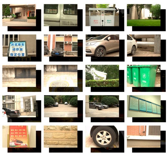
Figure 7.
All images in our dataset. Normal-light images (ground truth) are shown at the front. The low-light images (extremely dark) are shown behind.
Table 2.
The EXIF parameters of the training images. The first ID column indicates the number of image pairs. The order of ID is from left to right of every line, then the next line, and so on. The second column EXIF indicates the photos’ parameters. GT = ground truth. All the parameters of the dark images are as same as that of GT except shutter time.
4. Experiments
4.1. Dataset
The images in our dataset were collected from real-world scenes instead of by the artificial brightness adjustment. The images in our training dataset were taken in a cloudy environment by a Nikon D700 made in Japan. The lens was the fixed-focus lens labeled as AF-S NIKKOR 50 mm f/1.4G. Because the RAW format can save more low-light information than the sRGB format, the images were saved in the RAW format. The data collection environments of various algorithms are shown in Table 3. The dataset was divided into the training data and the test data. All the training images were taken outdoors and selected randomly from the image pairs. The training data included the 20 image pairs shown in Figure 7. To avoid overfitting, the test images were taken separately in the low-light environment and independent of the training data. The test images were taken from a variety of scenes, such as a bedroom and outdoors. They were taken from the environment about 1 lumen, approximately 100 times lower brightness than that of the training images. Some of the test images are shown in Figure 8. The exposure time of the training pictures was reduced exactly 100 times compared to the test data picture. The training images and test images were independent and identically distributed (i.i.d.) to guarantee the effectiveness of our algorithm.
Table 3.
The environments of collecting images in various algorithms.
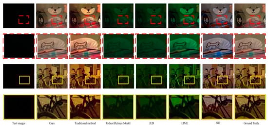
Figure 8.
The results of the various algorithms. The images marked with a red dotted box on the second row are the zoom-in images of the region surrounded by the small red dotted box in line 1, respectively. The images surrounded by the orange boxes in the fourth line are also the magnified images from the solid orange box region in line 3. The indoor test image (upper left sub-image) was taken with the parameters: exposure compensation +1.0, f 6.1, 0.1 s and ISO 400. The outdoor test image (third line and first column) was taken with the parameters: f 3.5, 0.2 s and ISO 400. The first column shows the test images taken in an extremely dark condition. The second column shows our results by the end-to-end deep learning model. The third column shows the results by the traditional method which cascades luminosity scaling and BM3D [20]. The fourth to the seventh columns show the results by the Robust Retinex Model algorithm [36], by JED [37], by LIME [28] and SID [9]. The last column shows the ground truth taken with a long exposure time.
4.2. Qualitative Results and Perceptual Analysis
The methods as a comparative baseline include the traditional method and the “modern” method. The traditional method cascades a luminosity scaling algorithm and a denoising algorithm. BM3D was selected as the classic denoising algorithm in our research because it outperforms most techniques facing the images with real noise. The modern data-driven approach selects some machine learning algorithms that have been proposed in recent years.
The process of determining the level of image quality is called Image Quality Assessment (IQA). IQA is part of the quality of experience measures. Image quality can be assessed using two kinds of methods: subjective and objective. In the subjective method, the corresponding result images processed by different pipelines were presented to students, who determine which image had higher quality. The images were presented in a random order, with a random left–right order without any indication of the provenance. A total of 100 comparisons were performed by five students. The students found the results using the traditional method (the third column) still had a good aspect of light, but there were some yellow patches in the large white region and noise particles. Other “modern” algorithms [28,36,37] did not work well in the extremely dark real environments. Our results were superior in the aspects of the image contrast, color accuracy, dynamic range, and exposure accuracy. Our pipeline significantly outperformed the traditional method and the “modern” methods in the aspect of denoising and color collection, respectively. The results by the various algorithms are shown in Figure 8.
4.3. Quantitative Analysis
The objective IQA methods were used to quantitatively measure the results. The objective methods can be classified into full-reference (FR) methods, reduced-reference (RR) methods, and no-reference (NR) methods.
FR metrics try to assess an image quality by comparing it with a reference image (ground truth) that is assumed to have perfect quality. The classical FR methods, the peak signal-to-noise ratio (PSNR) and the structural similarity index (SSIM [38]) were selected in our quantitative analysis. The higher the value of the two FR methods, the better the image quality.
The ENIQA [39] and Integrated Local NIQE (IL-NIQE) [40] present the high-performance general-purpose NR IQA methods based on image entropy. IL-NIQE uses a feature-enriched completely blind image quality evaluator. NIQE [41] makes a completely blind image quality analyzer and is also one of the NR methods. SSEQ [42] evaluates image quality assessment based on spatial and spectral entropies without a reference image. The lower scores calculated by these NR methods represents better image quality.
The quantitative IQA of the experimental results is shown in Table 4 and Table 5. The size of the toy image in Table 4 was set to 512 × 339 pixels. The size of the bicycle image in Table 5 was set to 512 × 340 pixels. The images in the PNG format were evaluated by the following IQA algorithms, except SID [9]. The original model in SID only accepted the 16-bit raw image taken by the Sony camera and 14-bit raw image taken by the Fuji camera. Our test images were taken with a Nikon DSLR D700 made in Japan. Therefore, we modified the test code of SID to accept our test images.
Table 4.
The Image Quality Assessment (IQA) of the recovery results about the toy image. The first column shows the various IQA methods. The columns (from second to seventh) show the corresponding IQA scores of the image results by various algorithms. The last column shows the score of the ground truth. The bold font and “(1)” indicate the value that is the best score. The underline and “(2)” represent second place.
Table 5.
The IQA of the recovery results about the bicycle image. The first column shows the various IQA methods. The columns (from second to seventh) show the corresponding IQA scores of the image results by various algorithms. The last column shows the score of the ground truth. The bold font and “(1)” indicate the value that is the best score. The underline and “(2)” represent second place.
Similar to the qualitative assessment, our method also exceeds most methods in quantitative analysis. The Robust Retinex Model, JED, and LIME can achieve better effect in this degree of light at dusk, but these methods do not work in extremely dark environments.
Due to the lack of reference images, the NR methods do not know which image is the ground truth. By NIQE and SSEQ (Line 5 and Line 6), the scores of our result even are a little better than that of ground truth. The close scores of ours and ground truth calculated by NIQE mean that our restored images are well.
Next, we analyzed the generalization performance of the network model. The generalization performance of a learning algorithm refers to the performance on out-of-sample data of the models learned by the algorithm. The test images in Figure 8 were shot in an environment that is as bright as that of the training images. In this experiment, the test images were taken with different camera parameters in an extremely low-light environment by different parameters. The camera metering system indicated the setting (F5, 50 s, ISO 400) can achieve normal exposure. The test images with different levels of darkness were collected by only adjusting the shutter time. For example, the exposure time was set to 0.5 second to 100 × less exposure, as shown in the second column of Figure 7. Similarly, the exposure times were set to 1 s, 1/4 s, 1/8 s, and 1/15 s, which means 50×, 200×, 400×, and 750× less exposure, respectively.
The curves are smooth in the second line of Figure 9. However, some line deformation can be found in the fourth line of Figure 9. The details of the line illustrate that our method has more powerful capabilities to restore details than the traditional method. The sub-images from the first to third column show that our algorithm adapts to the environments with varying degrees of darkness. Even in extreme exposure condition (750× less exposure), our method can restore the acceptable details.
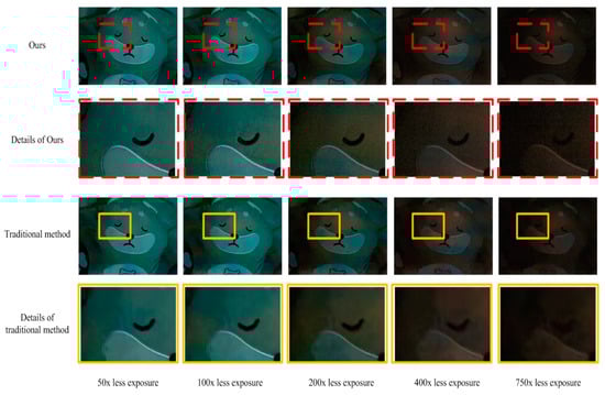
Figure 9.
The restoration results in different brightness environments. The first line shows the restoration results of the test images with different black levels by our algorithm. The second line shows the details of the results. The bottom two lines show the results handled by traditional methods. The columns represent the different original brightness levels.
In addition to subjective analysis, several objective IQA methods were adopted to evaluate image quality. The quantitative analysis of the effect of different exposures is shown in Table 6. It is obvious to see our method surpasses the traditional approach.
Table 6.
The IQA of the recovery results about the image with different exposures. In line 1, the word “n”× (“n” indicates a number) indicates n times reduction of exposure amount on the bases of normal exposure. The first column indicates the assessment methods and restoration algorithm. The traditional method is abbreviated as TM. Bold numbers represent the best results in this line. Underlined numbers indicate better results in different algorithms.
4.4. Implementation Details
In our study, the input images are the RAW images with the size H × W × 1. H and W are the abbreviations of the height and the width and are equal to 2832 and 4256, respectively. The input images were packed into four channels and correspondingly cut in half in each dimension. Thus, the size of the channels was 0.5 H × 0.5 W × 4. The packed data was fed into a neural network. Because the U-net network has a residual connection [43,44] and supports the full-resolution image in GPU memory, we selected a network with the architecture similar to U-net [10]. The output of the deep learning network was a 12-channel image with the size 0.5 H × 0.5 W × 12. Lastly, the 12-channel image was processed by a sub-pixel layer to recover the RGB image with the size H × W × 3.
Our implementation was based on TensorFlow and python. In all of our experiments, we used L1 loss, the Adam optimizer [45], and the Leaky ReLU (LRelu) [46] activation function. We trained the network for the Nikon D700 camera images. The initial learning rate was set to 0.0001, weight decay to 0.00001, and dampening to 0. The initial learning rate decreased according to the cosine function. According to the practical effect of the experiment, we set the training epoch as 4000.
5. Discussion
In this work, we shared a new collecting image method that can be used for future research on machine learning. Our algorithm was only trained with 20 image pairs and achieved the inspiring result in the restoration of the extremely low-light images with the help of a high-quality dataset. The method can be used in most supervised learning tasks.
In the future, we will try to improve our work in the following points. (1) It is known that Restricted Boltzmann Machines (RBMs) [47] can be used to preprocess the data and help the machine learning process become more efficient. The NL2LL model based on RMB might provide even better results. (2) Improved U-net networks can be used to improve performance. (3) The generalization performance of the method still needs to be studied. In our study, the recovered images were poor when the brightness of test images was magnified more than 400 times. Prior information about the environment light can be used for the algorithm. (4) The shooting environment can be extended to more complex scenarios, such as the condition with dark and blur and the condition with dark and scatting, etc. (5) The method can be used for low movement data (spatiotemporal data) and 3D objects (3D geometry).
Our research is of great significance in areas such as underwater robots and surveillance.
6. Conclusions
To see in the extreme dark, we have proposed a new method, NL2LL (collecting a low-light dataset in normal-light condition) to collect image pairs. The method has many potential implementations in convolutional neural network, dilated convolutional NN, regression, and graphical models. Our end-to-end approach is simple and highly effective. We have demonstrated its efficacy in low-light image restoration. The experiment shows that our approach can achieve inspiring results by only using 20 image pairs.
Author Contributions
All authors contributed to the paper. H.W. performed project administration; Y.X. conceived, designed and performed the experiments; Y.X. and G.D.C. wrote and reviewed the paper; S.R. performed the experiments; W.S. analyzed the data. All authors have read and agreed to the published version of the manuscript.
Funding
This research was funded by National Science Foundation of China (NSFC) grant No. 61571369. It was also funded by Zhejiang Provincial Natural Science Foundation (ZJNSF) grant No.LY18F010018. It was also supported by the 111 Project under Grant No. B18041.
Conflicts of Interest
The authors declare no conflict of interest.
References
- Hu, Z.; Cho, S.; Wang, J.; Yang, M.H. Deblurring low-light images with light streaks. In Proceedings of the IEEE Conference on Computer Vision and Pattern Recognition, Columbus, OH, USA, 24–27 June 2014; pp. 3382–3389. [Google Scholar]
- Remez, T.; Litany, O.; Giryes, R.; Bronstein, A.M. Deep Convolutional Denoising of Low-Light Images. arXiv 2017, arXiv:1701.01687. [Google Scholar]
- Zhang, X.; Shen, P.; Luo, L.; Zhang, L.; Song, J. Enhancement and noise reduction of very low light level images. In Proceedings of the 21st International Conference on Pattern Recognition (ICPR2012), Tsukuba, Japan, 11–15 November 2012. [Google Scholar]
- Plotz, T.; Roth, S. Benchmarking denoising algorithms with real photographs. In Proceedings of the IEEE Conference on Computer Vision and Pattern Recognition, Honolulu, HI, USA, 21–26 July 2017; pp. 1586–1595. [Google Scholar]
- Wang, R.; Zhang, Q.; Fu, C.W.; Shen, X.; Zheng, W.S.; Jia, J. Underexposed Photo Enhancement using Deep Illumination Estimation. In Proceedings of the IEEE Conference on Computer Vision and Pattern Recognition, Long Beach, CA, USA, 16–20 June 2019. [Google Scholar]
- Hasinoff, S.W.; Sharlet, D.; Geiss, R.; Adams, A.; Barron, J.T.; Kainz, F.; Chen, J.; Levoy, M. Burst photography for high dynamic range and low-light imaging on mobile cameras. ACM Trans. Graph. 2016. [Google Scholar] [CrossRef]
- Liu, Z.; Yuan, L.; Tang, X.; Uyttendaele, M.; Suny, J. Fast burst images denoising. ACM Trans. Graph. 2014. [Google Scholar] [CrossRef]
- Mildenhall, B.; Barron, J.T.; Chen, J.; Sharlet, D.; Ng, R.; Carroll, R. Burst Denoising with Kernel Prediction Networks. In Proceedings of the IEEE Conference on Computer Vision and Pattern Recognition, Salt Lake City, UT, USA, 18–22 June 2018. [Google Scholar] [CrossRef]
- Chen, C.; Chen, Q.; Xu, J.; Koltun, V. Learning to See in the Dark. In Proceedings of the IEEE Conference on Computer Vision and Pattern Recognition, Salt Lake City, UT, USA, 18–22 June 2018. [Google Scholar] [CrossRef]
- Ronneberger, O.; Fischer, P.; Brox, T. U-Net: Convolutional Networks for Biomedical Image Segmentation. In International Conference on Medical Image Computing and Computer-Assisted Intervention; Springer: Cham, Switzerland, 2015; pp. 234–241. [Google Scholar] [CrossRef]
- Everingham, M.; van Gool, L.; Williams, C.K.I.; Winn, J.; Zisserman, A. The pascal visual object classes (VOC) challenge. Int. J. Comput. Vis. 2010. [Google Scholar] [CrossRef]
- Russakovsky, O.; Deng, J.; Su, H.; Krause, J.; Satheesh, S.; Ma, S.; Huang, Z.; Karpathy, A.; Khosla, A.; Bernstein, M.; et al. ImageNet Large Scale Visual Recognition Challenge. Int. J. Comput. Vis. 2015. [Google Scholar] [CrossRef]
- Cheng, M.M.; Zhang, Z.; Lin, W.Y.; Torr, P. BING: Binarized normed gradients for objectness estimation at 300fps. In Proceedings of the IEEE Conference on Computer Vision and Pattern Recognition, Columbus, OH, USA, 23–28 June 2014. [Google Scholar] [CrossRef]
- Lore, K.G.; Akintayo, A.; Sarkar, S. LLNet: A deep autoencoder approach to natural low-light image enhancement. Pattern Recognit. 2017. [Google Scholar] [CrossRef]
- Xu, J.; Li, H.; Liang, Z.; Zhang, D.; Zhang, L. Real-World Noisy Image Denoising: A New Benchmark. arXiv 2018, arXiv:1804.02603. [Google Scholar]
- Wei, C.; Wang, W.; Yang, W.; Liu, J. Deep Retinex Decomposition for Low-Light Enhancement. arXiv 2018, arXiv:1808.04560. [Google Scholar]
- Loh, Y.P.; Chan, C.S. Getting to know low-light images with the Exclusively Dark dataset. Comput. Vis. Image Underst. 2019. [Google Scholar] [CrossRef]
- Rudin, L.I.; Osher, S.; Fatemi, E. Nonlinear total variation based noise removal algorithms. Phys. D Nonlinear Phenom. 1992. [Google Scholar] [CrossRef]
- Mairal, J.; Bach, F.; Ponce, J.; Sapiro, G.; Zisserman, A. Non-local sparse models for image restoration. In Proceedings of the 2009 IEEE 12th International Conference on Computer Vision, Kyoto, Japan, 29 September–2 October 2009. [Google Scholar] [CrossRef]
- Dabov, K.; Foi, A.; Katkovnik, V.; Egiazarian, K. Image denoising by sparse 3-D transform-domain collaborative filtering. IEEE Trans. Image Process. 2007. [Google Scholar] [CrossRef]
- Zhang, K.; Zuo, W.; Chen, Y.; Meng, D.; Zhang, L. Beyond a Gaussian denoiser: Residual learning of deep CNN for image denoising. IEEE Trans. Image Process. 2017. [Google Scholar] [CrossRef] [PubMed]
- Xie, J.; Xu, L.; Chen, E. Image denoising and inpainting with deep neural networks. Adv. Neural Inf. Process. Syst. 2012. [Google Scholar] [CrossRef]
- Łoza, A.; Bull, D.; Achim, A. Automatic contrast enhancement of low-light images based on local statistics of wavelet coefficients. In Proceedings of the 2010 IEEE International Conference on Image Processing, Hong Kong, China, 26–29 September 2010. [Google Scholar] [CrossRef]
- Burger, H.C.; Schuler, C.J.; Harmeling, S. Image denoising: Can plain neural networks compete with BM3D? In Proceedings of the 2012 IEEE Conference on Computer Vision and Pattern Recognition, Providence, RI, USA, 16–21 June 2012. [Google Scholar] [CrossRef]
- Joshi, N.; Cohen, M.F.; Seeing, M.T. Rainier: Lucky imaging for multi-image denoising, sharpening, and haze removal. In Proceedings of the 2010 IEEE International Conference onComputational Photography (ICCP), Cambridge, MA, USA, 29–30 March 2010. [Google Scholar] [CrossRef]
- Ignatov, A.; Kobyshev, N.; Timofte, R.; Vanhoey, K.; van Gool, L. WESPE: Weakly supervised photo enhancer for digital cameras. In Proceedings of the IEEE Conference on Computer Vision and Pattern Recognition Workshops, Salt Lake City, UT, USA, 18–22 June 2018. [Google Scholar] [CrossRef]
- Dong, X.; Wang, G.; Pang, Y.; Li, W.; Wen, J.; Meng, W.; Lu, Y. Fast efficient algorithm for enhancement of low lighting video. In Proceedings of the 2011 IEEE International Conference on Multimedia and Expo, Barcelona, Spain, 18–15 July 2011. [Google Scholar] [CrossRef]
- Guo, X.; Li, Y.; Ling, H. LIME: Low-light image enhancement via illumination map estimation. IEEE Trans. Image Process. 2017. [Google Scholar] [CrossRef] [PubMed]
- LeCun, Y.; Boser, B.; Denker, J.S.; Henderson, D.; Howard, R.E.; Hubbard, W.; Jackel, L.D. Backpropagation Applied to Handwritten Zip Code Recognition. Neural Comput. 1989, 1, 541–551. [Google Scholar] [CrossRef]
- le Cun, Y.; Fogelman-Soulié, F. Modèles connexionnistes de l’apprentissage, Intellectica. Rev. l’Association Pour Rech. Cogn. 1987. [Google Scholar] [CrossRef]
- Hinton, G.E.; Zemel, R.S. Autoencoders Minimum Description Length and Helmholtz free Energy. Adv. Neural Inf. Process. Syst. 1994. [Google Scholar] [CrossRef]
- Poggio, T.; Torre, V.; Koch, C. Computational vision and regularization theory. Nature 1985. [Google Scholar] [CrossRef]
- Friedman, J.H. Regularized discriminant analysis. J. Am. Stat. Assoc. 1989. [Google Scholar] [CrossRef]
- Vincent, P.; Larochelle, H.; Bengio, Y.; Manzagol, P.A. Extracting and composing robust features with denoising autoencoders. In Proceedings of the 25th International Conference on Machine Learning, Helsinki, Finland, 5–9 July 2008. [Google Scholar] [CrossRef]
- Goodfellow, A.C.I. Yoshua Bengio, Deep Learning Book. Deep Learn. 2015. [Google Scholar] [CrossRef]
- Li, M.; Liu, J.; Yang, W.; Sun, X.; Guo, Z. Structure-Revealing Low-Light Image Enhancement Via Robust Retinex Model. IEEE Trans. Image Process. 2018. [Google Scholar] [CrossRef]
- Ren, X.; Li, M.; Cheng, W.H.; Liu, J. Joint enhancement and denoising method via sequential decomposition. In Proceedings of the 2018 IEEE International Symposium on Circuits and Systems (ISCAS), Florence, Italy, 27–30 May 2018; pp. 1–5. [Google Scholar]
- Wang, Z.; Bovik, A.C.; Sheikh, H.R.; Simoncelli, E.P. Image quality assessment: From error visibility to structural similarity. IEEE Trans. Image Process. 2004. [Google Scholar] [CrossRef] [PubMed]
- Chen, X.; Zhang, Q.; Lin, M.; Yang, G.; He, C. No-reference color image quality assessment: From entropy to perceptual quality, Eurasip. J. Image Video Process. 2019. [Google Scholar] [CrossRef]
- Zhang, L.; Zhang, L.; Bovik, A.C. A feature-enriched completely blind image quality evaluator. IEEE Trans. Image Process. 2015. [Google Scholar] [CrossRef] [PubMed]
- Mittal, A.; Soundararajan, R.; Bovik, A.C. Making a “completely blind” image quality analyzer. IEEE Signal Process. Lett. 2013. [Google Scholar] [CrossRef]
- Liu, L.; Liu, B.; Huang, H.; Bovik, A.C. No-reference image quality assessment based on spatial and spectral entropies. Signal Process. Image Commun. 2014. [Google Scholar] [CrossRef]
- He, K.; Zhang, X.; Ren, S.; Sun, J. Deep Residual Learning for Image Recognition. In Proceedings of the 2016 IEEE Conference on Computer Vision and Pattern Recognition, Las Vegas, NV, USA, 27–30 June 2016. [Google Scholar] [CrossRef]
- Xu, Y.; Wang, H.; Liu, X. An improved multi-branch residual network based on random multiplier and adaptive cosine learning rate method. J. Vis. Commun. Image Represent. 2019, 59, 363–370. [Google Scholar] [CrossRef]
- Kingma, D.P.; Ba, J.L. Adam: A method for stochastic optimization. arXiv 2015, arXiv:1412.6980. [Google Scholar]
- Xu, B.; Wang, N.; Chen, T.; Li, M. Empirical Evaluation of Rectified Activations in Convolutional Network. arXiv 2015, arXiv:1505.00853. [Google Scholar]
- Salakhutdinov, R.; Mnih, A.; Hinton, G. Restricted Boltzmann machines for collaborative filtering. In Proceedings of the 24th International Conference on Machine Learning, Corvalis, OR, USA, 20 June 2007; pp. 791–798. [Google Scholar]


© 2020 by the authors. Licensee MDPI, Basel, Switzerland. This article is an open access article distributed under the terms and conditions of the Creative Commons Attribution (CC BY) license (http://creativecommons.org/licenses/by/4.0/).