Experimental and Model-Based Study of the Vibrations in the Load Cell Response of Automatic Weight Fillers

Abstract

The paper presents a study of the vibrations in the load cell response of automatic weight fillers for fluids, due to the dynamics of the system. The aim is to characterize vibratory phenomena through both experimental and model-based analysis, in order to identify the main causes and identify compensation strategies. Two test campaigns were conducted, on a test bench and on a sixteen stations machine, with the simultaneous acquisition of acceleration signals and load cell signals. A detailed sensitivity analysis based on experimental data, as many system parameters vary, has been developed. For the system modelling, a one Degree of Freedom (1 DoF) model, with lumped parameters and time-variant mass, including fluidic forces, was considered and numerically implemented. Genetic algorithms were used for the identification problems in the model-based analysis. The model allowed a deeper understanding of the phenomena that occur, showing promising results for the vibration prediction in a compensation process.

1. Introduction

In the consumer goods industries, a common task is to fill bottles with an exact quantity of liquid (juice, water, oil, drink, detergent, etc.). The filling process is sometimes performed with a continuous control of the net weight of the dispensed product, in other cases with a flow rate control. In the first case, the machine that carries out the filling is called the weight filler, whereas, in the second case, it is called the volumetric filler. Weight fillers assure that the quantity of product injected into the container satisfies the requirements with a gram order tolerance, and they can be customized for different volumes and sizes of bottles. For the weighing task, commonly used sensors are single-point strain gauge load cells, widely diffused in industrial applications (checkweighers, catchweighers, weight-price labelers, multi-head weighers, etc.). The fundamental performance for weight filling machines is their accuracy in filling and short cycle times. Typically, operation variables (e.g., filling flow-rate), environmental conditions (e.g., temperature, humidity), fluid properties (e.g., viscosity) and vibrations of the mechanical components affect the weighing process. Vibration assessment is a critical issue for weight fillers, in fact in the dynamic weighing process, a definitive measure can only be achieved when a stable equilibrium is achieved [1,2,3,4]. A filling problem widely studied in the literature concerns vibratory phenomena and their effect on low-dose capsules’ filling (e.g., [5,6]), but few works deal with liquid filling machines [7]. Rotary weight filler machines are generally moved at very high speed, having to carry out the filling in a very short time and are inserted in a system with other machines, therefore reliability is an extremely important issue.

The condition monitoring problem of these machines has been widely studied, often with artificial intelligence-based approaches [8,9,10]. Sensor response is often influenced by low frequency vibrations induced by the oscillatory behavior of the load cell and by environmental vibrations (also called “floor” vibrations). The common approach, consisting in correcting the measured signal by filtering the high frequency Fourier components (low-pass filters), in such cases may not be effective. The floor vibrations are associated with excitations caused by internal (inertial) or external (impacts) vibration sources, combined with the flexibility of the machine frame. To overcome the limitations associated with the correction of the load cell response with low-pass filters, many solutions have been proposed in literature [11,12]. A model-based approach, experimentally validated, is proposed in [13], for the compensation of the environmental vibrations transmitted by the elastic frame. An interesting use of load cell-based weight measurement is the dynamic weighing calibration of liquid flowmeters [14,15]. An innovative approach in the dynamic weighing approach proposed by the authors permits the reduction of the calibration time, energy cost and workload in liquid flow calibration laboratories. Instead, the analysis of the interaction between the dynamics of the weighing system and the forces induced by the flow is the basis of the proposed approach.

This work proposes a theoretical and an experimental study of the vibrations in a weight filler. Experiments carried on a dedicated test-bench, on a sixteen stations machine and on a forty-four stations machine in different working conditions, by achieving load-cell and accelerometer measures, allowed the performance of a sensitivity analysis of the vibration phenomena. The fluid, the tank filling level, the delivered mass and the distance between the dispenser and the support plate of the bottle have been varied to study how the load cell measurement is affected by them. A theoretical analysis, based on a one degree of freedom spring-damper with variable mass model, has been considered to study the dynamics of the weighing process and to develop a method for predicting vibratory phenomena. This model-based approach was applied for the first time by the authors [8] to the problem of dynamic weighing in filling machines, where the mass is time-variant. An extension is presented in this article, with a reformulation of the model and by implementing an automatic identification methodology of model parameters and mass flow rate, based on the use of Genetic Algorithms (GA). From the analysis of the new results, a deeper understanding of the phenomena that occur has been achieved. The adopted model is similar to that presented in [15], but it has been opportunely adapted to a different use: the buoyancy force has been neglected, since it may be considered irrelevant in the considered system, and the problem formulation has been changed to fit the purpose. In [15], the model is used for a hydrodynamic force correction to enhance the flow measurement accuracy; in the current paper, the aims are the identification of the potential sources of vibrations, for a possible elimination and a prediction of vibratory phenomena for compensation. The dynamic effects of flow-induced forces are implemented in the model. The data collected in the experimental tests have been used to identify the model parameters, the possible flow pattern and the internal disturbing forces that arise due to impulses introduced by machine elements (such as the valve for the flow circulation opening and closing). Furthermore, GA are used for the optimization problem of the identification.

The paper is organized as follows. The experimental study of the vibrations is presented in Section 2: Section 2.1 describes the weight filler machines and their operation mode; Section 2.2 is devoted to presenting the experimental tests and the results of the analyses carried out. Section 3 illustrates the model-based analysis of the vibratory phenomena: Section 3.1 describes the mechanical model of the system, characterized by variable mass; Section 3.2 depicts the results of the implementation of the model, applied to the experimental tests. Finally, concluding remarks are provided in Section 4.

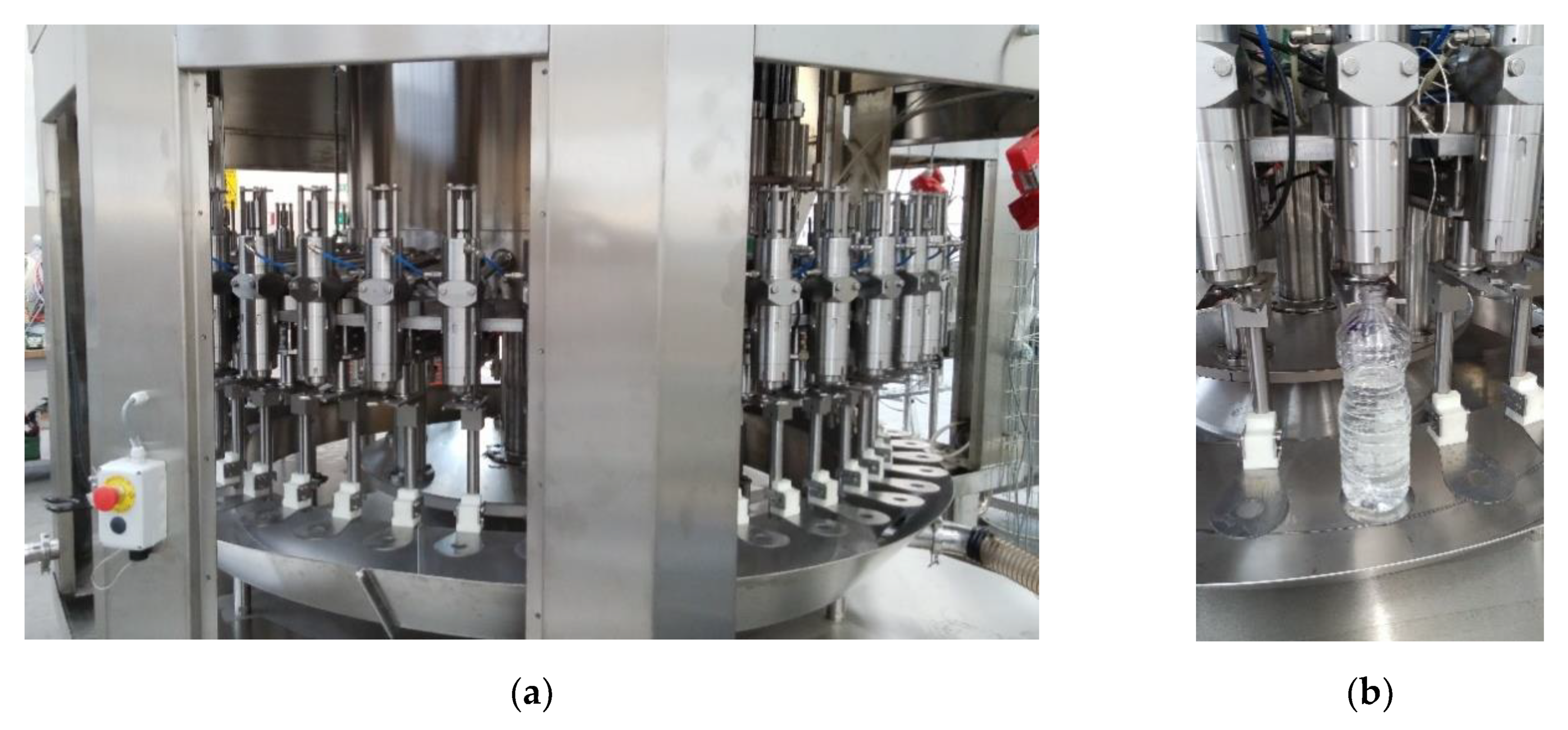
2. Experimental Study of the Filling Process

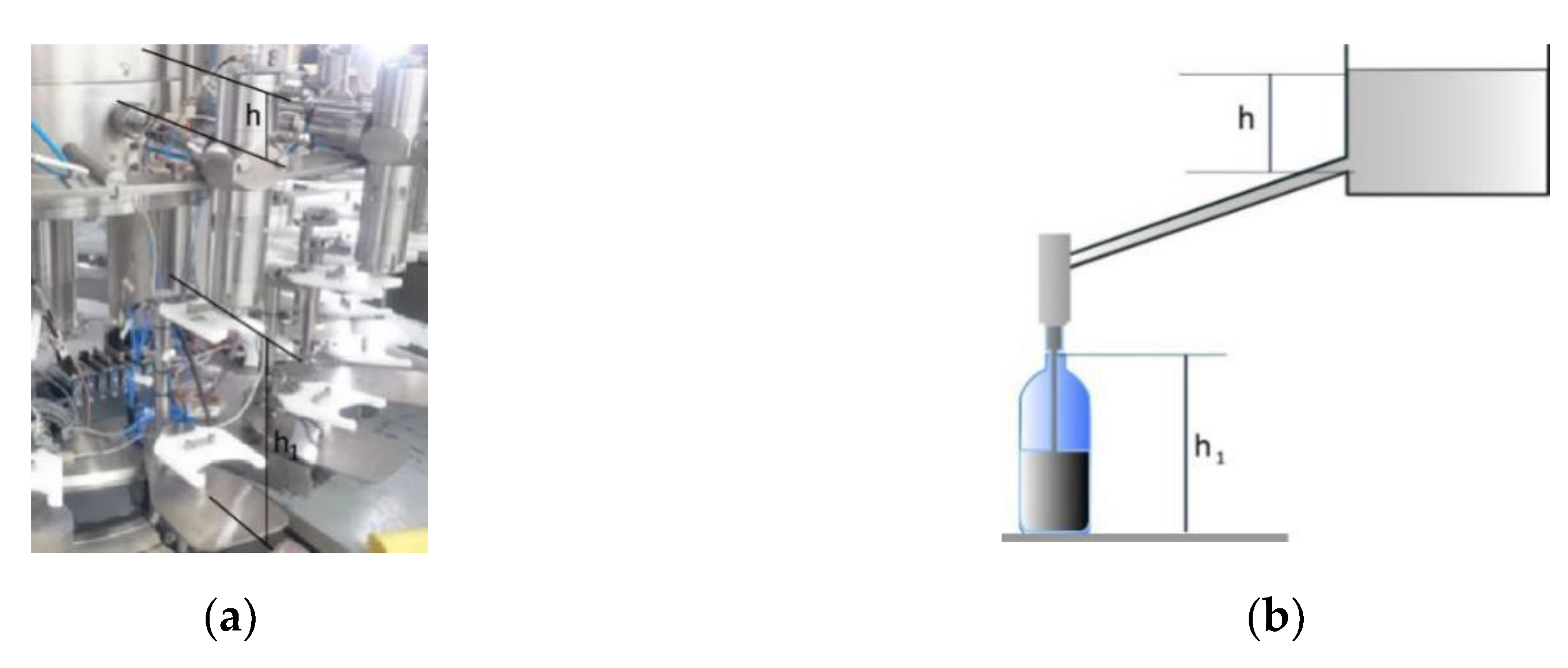
2.1. Weight Filling Process

Automatic filling machines deliver an exact quantity of fluid, powder or sauce into a bottle or, more generally, into a container. The filling operation often requires an aseptic environment, particularly in the food or pharmaceutical industry. A Human Machine Interface (HMI) or a remote controller allows the user to set the process parameters, such as the filling velocity or the quantity of the supplied product, assuring flexibility and high rates in the change of production volumes or formats. Among the various kinds of filling machines used in industry, this study was devoted to weight fillers for liquid in bottles, in which the filling process is performed with a continuous control of the net supplied weight. They were composed of a carousel with several stations (Figure 1). In each station, a support structure for the bottle, provided with a plate, managed the filling of the single bottle. A load cell, to measure tare and net weight of the filled product, was mounted under the plate and a bypass valve, connected upstream to the tank and downstream to the dispenser, allowing the filling of the bottle (Figure 1).

The filling process starts with loading the empty bottle on the machine using a conveyor belt and a rotating carousel; during the main carousel rotation, the bottle is filled. Successively, a third carousel and another conveyor belt allow the knockout of the filled bottle. During the filling, the bottle is opportunely constrained to the support structure through a clamping system and it is placed on the plate to measure the weight. For each loaded bottle, an automatic reset of the tare is performed, then, the filling is realized, continuously monitoring the weight, and the final value is checked. The tolerance to consider a filling in compliance with the specifications is of the gram order, or in some cases, less than a gram. The bottles with a final weight out of tolerance are rejected. The filling process can be schematized into four consecutive phases, corresponding to the four sectors with angular amplitude α, β, γ and δ, respectively (Figure 2).

• Tare weight measurement: The bottle enters the filling machine through the input-carousel and it is hooked to the plate support. During the α angle, the main carousel rotation occurs and the load cell weights the tare.
• Filling process: At the end of the α angle, the control system commands to open the bypass valve, starting the filling. The time corresponding to the β angle is automatically evaluated by the controller, also considering the product quantity that drops after the valve closing.
• Final weighing: During the γ angle, the final weight is measured. The bottle containers with a non-compliant weight are guided out of the carousel, such that an operator can remove them.
• Zero condition reset. During the δ angle, the check of the zero condition of the load cell is performed, in order to avoid a drift in the value read by the measuring system.

Mechanical stops prevent the overload of the load cell, avoiding its permanent deformation. A central controller constantly monitors the load cell measurement, assuring the control of the supplied product through the bypass valve. In the studied machine, the bypass valve is a pneumatic valve. It can also be provided with a device that avoids the creation of foam for foaming products. The amplitudes of the angles, α, γ and δ, may strongly affect the value of β and, as a consequence, the productivity of the weight filler. The second column of each sub-picture of Figure 2 reports samples of the acquired signals of the load cell (yellow) and of the acceleration of the plate in the vertical direction (light blue). The signal portion for each phase is highlighted by a grey rectangle. The signals show that the system dynamics are heavily influenced by the contribution of vibrational phenomena introduced on the system by repetitive abrupt events happening within each cycle. The mode of operation of the machine involves three certain abrupt events:

(1)

Loading the bottle into the station: generates an abrupt change of the weight read by the load cell reads as an impulse. The time associated with the α angle must allow the complete damping of the vibration;

(2)

Closing of the bypass valve at the end of the filling: generates a discontinuity in the forces applied to the load cell and a consequent vibration;

(3)

Unloading the bottle from the station: creates a high discontinuity on the load cell. The consequent vibration must be promptly damped, so that the zero position can be reset and the new cycle can start.

The presence of these vibrational phenomena represents a critical issue for the optimal functioning of the weight filler; for this reason, an experimental campaign is proposed for the characterization of the machine dynamics.

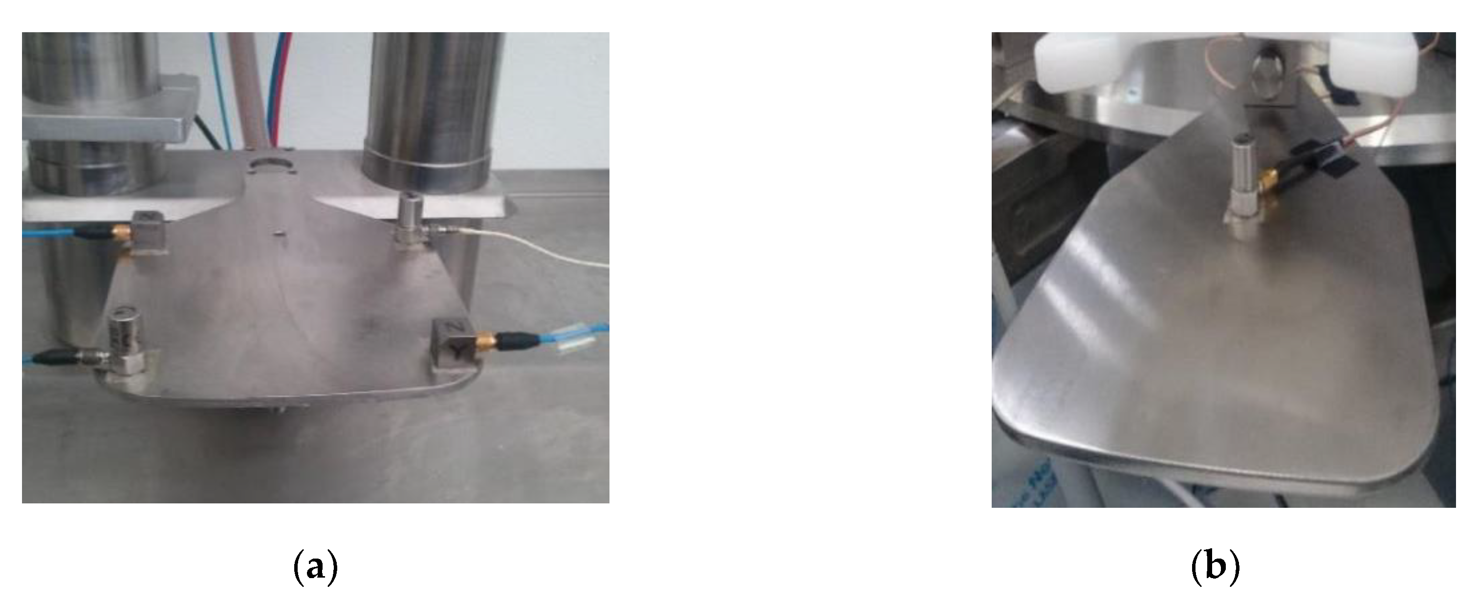
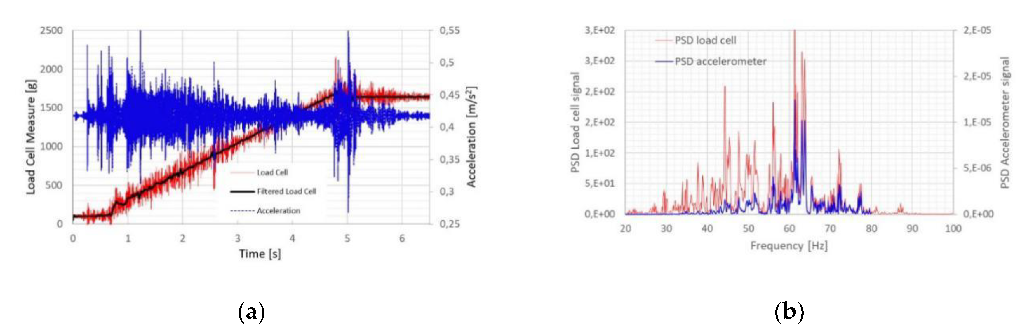
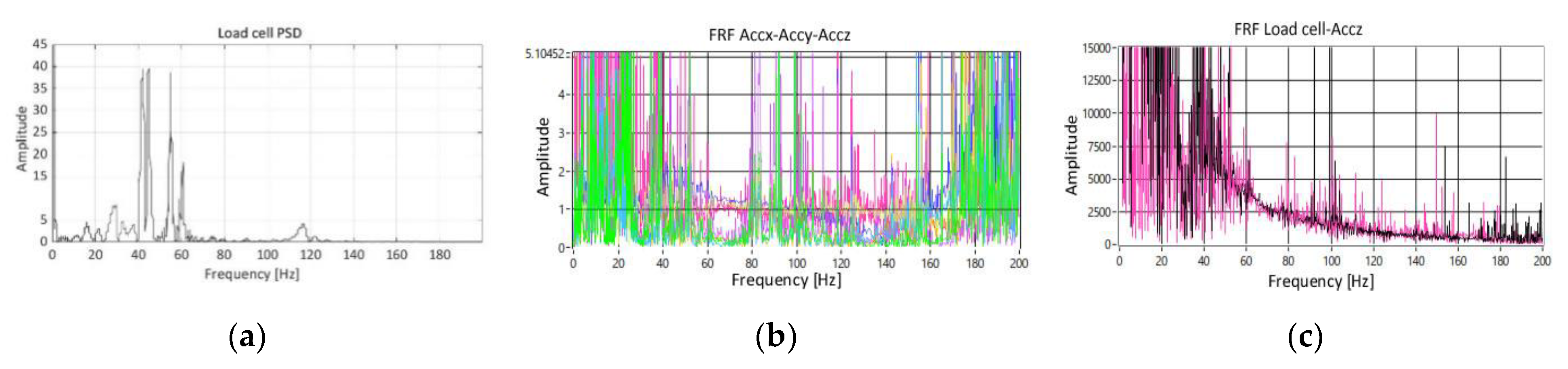
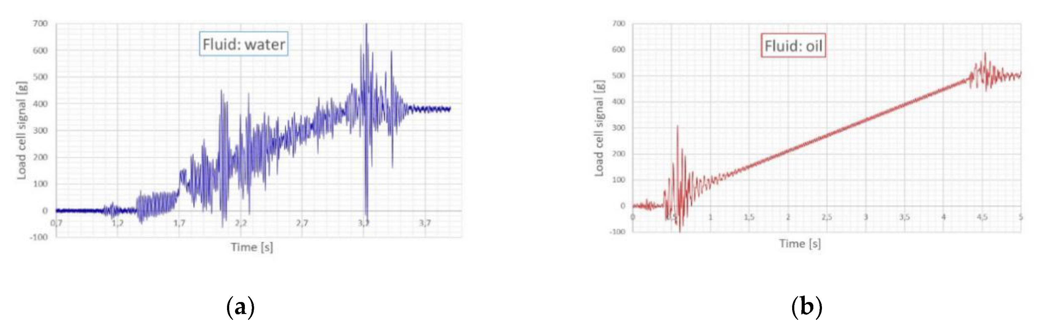
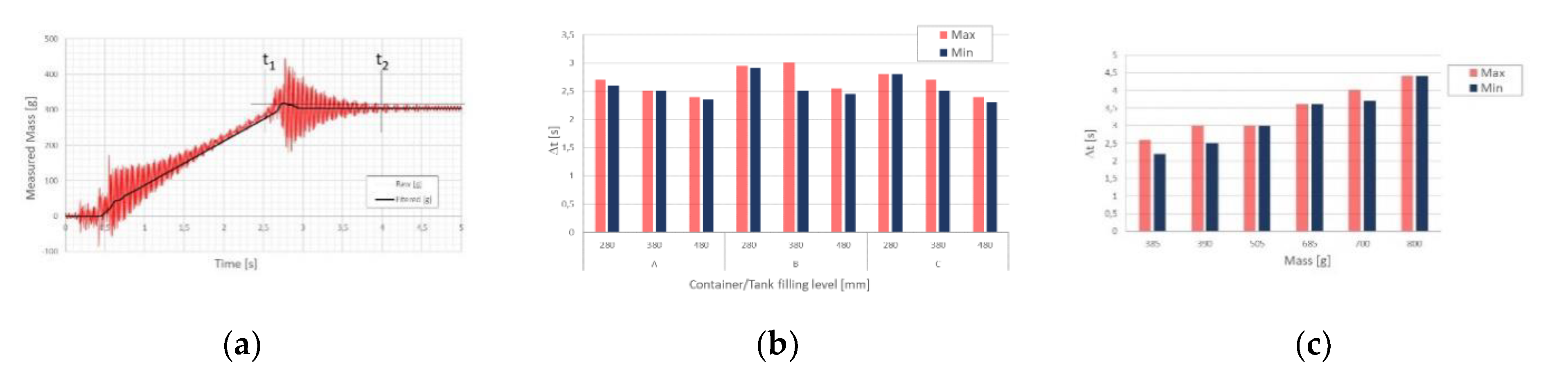
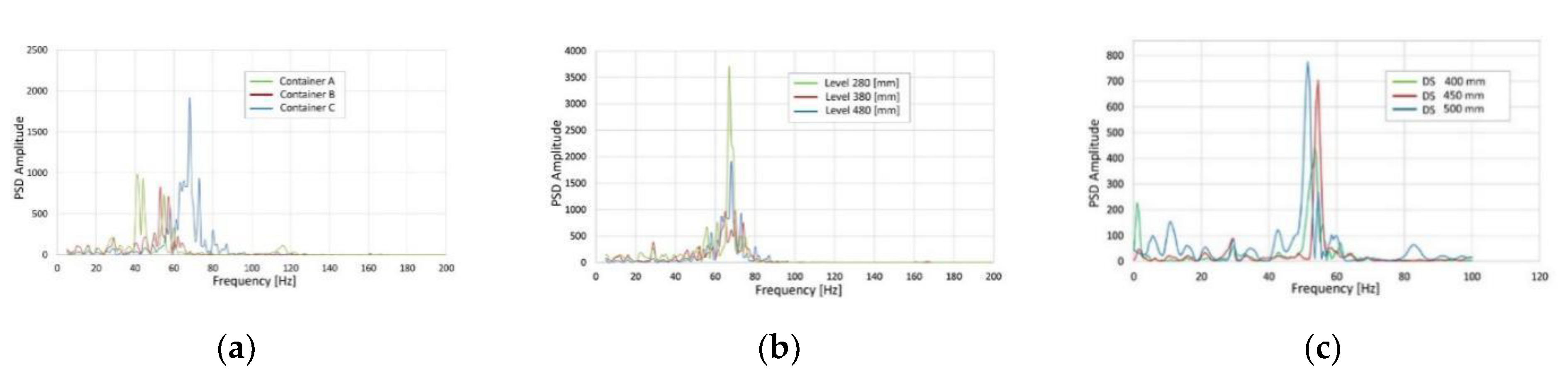
2.2. Experimental Analysis of Vibrations

The study was focused on the vibrations of the load cell measurements that interfere with the weighing phases (zero reset, tare, final net weighing), resulting in a longer measurement time. An experimental analysis can be useful to identify the main causes of these phenomena in order to try to compensate for them. The purpose of the measurements was to study the influence of the process parameters on the amplitude and frequencies of vibrations that affect the load cell signal. The phases of the filling process considered in the analysis were phases b (filling) and c (final weighing), as shown in Figure 2. Two test campaigns were carried out using a test-bench and a complete machine with sixteen stations. The test-bench repeated a single filling station and consisted of a tank, a bypass valve, a dispenser, a plate and a load cell. It was particularly suitable for studying the physical phenomena related to the delivery of a mass of fluid.

In the test campaign, on the test-bench, four accelerometers (two mono-axial and two tri-axial) were mounted on the plate, as shown in Figure 3a. The adopted configuration allows verification of whether there are disturbances in directions different from the vertical one (direction of the fluid fall), by comparing the signals of the cell with those of the accelerometers, more precise and with greater sensitivity. In the tests of the second campaign (on the weight filler), a mono-axial accelerometer was mounted on the plate (Figure 3b). The load cell used in all the tests was fixed under the plate; the model used is PW15PH type HBM with bridged strain gauges, with technical performances similar to those of the cells used on industrial machines. The acquisitions of the accelerometers and load cell measurements were carried out at a 10.240 kHz sampling frequency, using National Instruments instrumentation (NI 9172, cRIO, cDAQ 9191, NI 9233, NI 9237, NI 9219, NI 9215, NI 9218). The DAQ operates in a range of ±5 V with a 24-bit resolution. The mono-axial and tri-axial piezo-accelerometers with integrated electronics (IEPE/ICP) used during the tests sessions were the following (sensitivity is shown in brackets): mono-axial Wilcoxon Research mod.736 (100 mV/g), mono-axial Wilcoxon Research mod.732a (10 mV/g), mono-axial ultralight (0.3–0.8 mV/g), three-axial PCB Piezotronics mod.356A45 (100 mV/g).

Figure 4a reports the load cell (red signal) and the mono-axial accelerometer signals (blue-signal) for a test on the test-bench. Figure 4b shows the Power Spectral Density (PSD) of the two signals. Looking at the graphs, it is noted how the perturbations recorded by the load cell and the accelerometer were comparable and synchronous. From the test campaign 1, the transversal movement components can be evaluated by using tri-axial accelerometers. The results highlight that the most excited frequencies of cell and plate between 60 and 80 Hz (Figure 5a) did not match particular vibration modes of the structure. In this range of frequencies, the vertical component of acceleration was significant, whereas the components in other directions were negligible (Figure 5b). The relationship between the load cell signal and the vertical acceleration signals was almost constant, reflecting the fact that the movement was rigid (see the Frequency Response Function (FRF) in Figure 5c). Thus, the vibrations recorded on the load cell were effectively representative of the vertical movement of the plate and the other components are filtered by the cell itself. The data collected during the test campaigns show that, during the opening and closing phases, managed by a pneumatic valve, the impact of the valve spool on the valve body generated an oscillation on the cell signal, creating resonance. This behaviour was very evident in some tests, such as the one related to the graph of Figure 6a, in which at the instant of 1.35 s, the valve opened and, at the instant of 3.35 s, it closed. The signal of the load cell of Figure 6a refers to a test in which the fluid was water, while Figure 6b reports the signal of a test with oil. As expected, the water-related signal was affected by a noise component greater than that of the oil, for which there was a greater damping of the vibrations. The viscosity of the dispensed liquid had a considerable influence on the load cell signal. For this reason, subsequent tests were conducted with water. The incidence of some process parameters on the vibration phenomena was also studied. The parameters that varied in the test sessions were: tank filling level (h), delivered mass, type and shape of the container and distance between the dispenser and the plate ($h_1)$. The distances $h$ and $h_1$ are shown in Figure 7. In particular, the impact of these parameters on the damping time ($\Delta t)$ of the end-filling vibration, and on the excited frequencies, was analyzed.

Figure 8a shows how the damping time ($\Delta t=t_2-t_1$) was estimated: the time $t_1$ was taken at the moment in which the signal (in the last part of the filling) came out of a tolerance range for the first time, whereas $t_2$is the instant in which it returned with certainty in the defined threshold interval. Within a high number of tests and repetitions, the minimum and maximum values of $\Delta t$ have been evaluated. Tests with three containers of different shape, A, B and C, and different tare values (107.7 g, 394.4 g and 619.7 g, respectively), were performed.

At the end of the filling process, the load cell signal was affected by a vibration of very high amplitude, which required a significant time to dampen; this phenomenon is particularly evident in the signal of Figure 8a. In order to consider the measurement reliable, it was therefore necessary to wait for the time necessary for this vibration to fade. The time $t_2$ identifies the instant in which the weight can be considered stable and the load cell can send the final value. The Power Spectral Density (PSD) analysis has allowed the identification of the most excited frequencies. From the tests, it emerged that the geometry of the container does not clearly affect Δt, which instead varies significantly with the tank filling level (Figure 8b). The increase in the delivered mass determined the rise of Δt, as shown in Figure 8c. As the tare weight of the container increased (from container A to C), the excited frequencies moved towards lower values, as shown in Figure 9a (as it is reasonable to expect).

The increase in the tank filling level did not affect the excited frequencies, but did affect the amplitude of the oscillations (Figure 9b): this means that the amplitude of the vibrations varies if the filling level of the tank is lowered. The increase in the distance between the dispenser and the plate ($h_1$) determined an increase (quite limited) of Δt, which, for instance, corresponded to 3.72 s, 3.82 s and 3.9 s for distances of 400 mm, 450 mm and 500 mm, respectively. In fact, as $h_1$increased, the impact velocity rose and, consequently, the amplitude of the vibration, but the excited frequencies did not vary significantly (Figure 9c).

3. Model-Based Study of the System

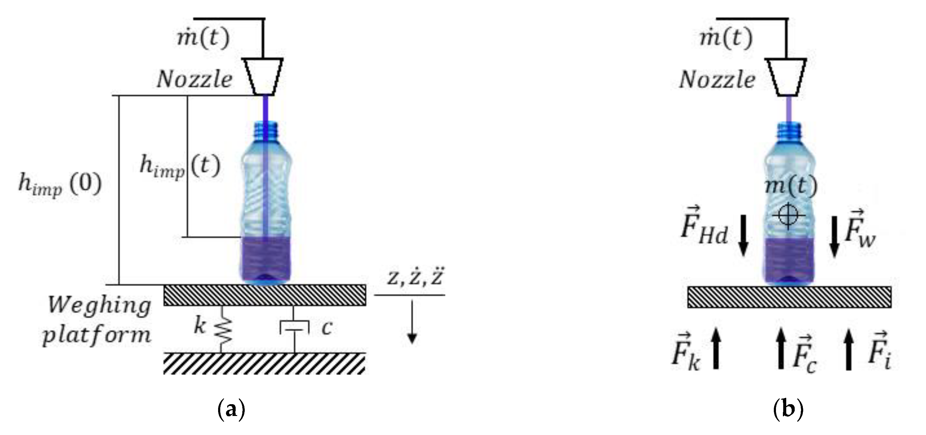
3.1. Modelling of the System

A mathematical model can be used to simulate the filling weighing process, for a better understanding of the involved phenomena. A one Degree of Freedom (1 DoF) numerical model, with lumped parameters and time-variant mass, can be obtained by applying the second dynamic principle in the axis of weighing (the vertical direction). The mass-spring-damping model is schematized in Figure 10a with the adopted notation; Figure 10b shows the forces applied to the mass. In the hypothesis of transversal components of insignificant force (as highlighted in Section 2.2) and of a linear behaviour of load cell and strain gauge, the model considered represents the best compromise between complexity and performance [12]. The total mass (m) of the fluid in the vessel is time variant during the filling, with the dependence on time expressed in (1) by denoting M₀ the total mass of the system with an empty vessel, and μ(t) the mass flow rate.

$$m\left(t\right)=M_0+\mu \left(t\right)·t$$

(1)

With the notation of Figure 10a, the speed of the mass $m\left(t\right)$ is $\dot{z}\left(t\right).$ Let $v\left(t\right)$ denote the speed of the infinitesimal mass $dm$. By applying the Newton law, in Euler’s form (in scalar notation), to the mass, Equation (2) can be written, where $F_{ext}$ is the result of external forces applied to mass $m$.

$$m\left(t\right)\frac{d}{dt}\left[\dot{z}\left(t\right)\right]+\left(\dot{z}\left(t\right)-v\left(t\right)\right)\frac{d}{dt}\left[m\left(t\right)\right]=F_{ext}\left(t\right)$$

(2)

The term $v\left(t\right)-\dot{z}\left(t\right)$ is the relative speed of the infinitesimal mass $dm$ with respect to mass m, that is the impact speed ($v_{imp}\left(t\right))$ of the jet of water normal to the surface of the liquid in the vessel. Equation (2) can be rewritten in the following form:

$$m\left(t\right)\frac{d}{dt}\left[\dot{z}\left(t\right)\right]=F_{ext}\left(t\right)+v_{imp}\left(t\right)\mu \left(t\right)$$

(3)

where the term $v_{imp}\left(t\right)\mu \left(t\right)$ is the hydrodynamic force ($\overrightarrow{F_{Hd}})$ (15) caused by the impact of the falling water jet upon the vessel bottom at the beginning of the filling, and afterwards upon the water surface. The velocity $v\left(t\right)$ of the flux at the point of contact with the water surface can be calculated by applying Bernoulli’s law, obtaining the $v_{imp}\left(t\right)$ expression in Equation (6), where $v_n\left(t\right)$ is the value of the velocity of the falling water at the nozzle outlet, and $h_{imp}\left(t\right)$ is the instantaneous impact height.

$$v_{imp}\left(t\right)=\sqrt{2·g·h_{imp}\left(t\right)+v_n{}^2\left(t\right)}-\dot{z}\left(t\right)$$

(4)

The impact height $h_{imp}\left(t\right)$ and the velocity $v_n\left(t\right)$ are function of the mass-flow rate as reported in Equation (5), where $A_n\left(t\right)$ is the nozzle outlet area, $A_v\left(t\right)$ is the vessel area, ${\rho }_f$ the fluid density and $h_i\left(0\right)$ the initial impact weight.

$$h_{imp}\left(t\right)=h_{imp}\left(0\right)-\frac{\mu \left(t\right)·t}{{\rho }_f·A_v} v_n\left(t\right)=\frac{\mu \left(t\right)·t}{{\rho }_f·A_n}$$

(5)

The external forces applied to the system are: the weight force ($\overrightarrow{F_w}$), which varies over time with the mass m(t), the elastic and the damping contributions ($\overrightarrow{F_k}$ and $\overrightarrow{F_c}$, respectively) introduced by the weighing system, with damping coefficient $c$ and stiffness coefficient $k$, and the buoyancy force, related to the floating effect that the air has upon the water volume. The latter force can be neglected compared to the others because it depends on the ratio ${\rho }_a/{\rho }_f$ (very close to zero) and on the mass, which in this case is limited; therefore it assumes much lower values than the other forces. By introducing the external forces in Equation (5), with the appropriate signs according to their verse, the motion equation becomes:

$$m\left(t\right)\frac{d}{dt}\left[\dot{z}\left(t\right)\right]+\left(c+\mu \left(t\right)\right)·\dot{z}\left(t\right)+k·z\left(t\right)=m\left(t\right)g+\mu \left(t\right)\sqrt{2·g·h_{imp}\left(t\right)+v_n{}^2\left(t\right)}$$

(6)

The second order linear-time-variant differential equation, which states the vertical dynamics of the system, can be rewritten in the form of Equation (7), where the natural frequency ${\omega }_N$ and the damping ratio ξ are clarified in Equation (8).

$$\ddot{z}\left(t\right)+2\xi \left(t\right){\omega }_N^2\left(t\right)·\dot{z}\left(t\right)+{\omega }_N^2\left(t\right)·z\left(t\right)=g+\mu \left(t\right)\sqrt{2·g·h_{imp}\left(t\right)+v_n{}^2\left(t\right)/m\left(t\right)}$$

(7)

With:

$${\omega }_N\left(t\right)=\sqrt{\frac{k}{m\left(t\right)}} \xi \left(t\right)=\frac{\mu \left(t\right)+c}{2\sqrt{m\left(t\right)·k}}$$

(8)

The analytical model was implemented in a software application developed in the Delphi environment and with a custom made MATLAB script (MATLAB Release 2018b, The MathWorks, Inc., Natick, MA, USA). A closed-form solution of the ODE was not available and a Runge-Kutta 4th order numerical method was used to solve it.

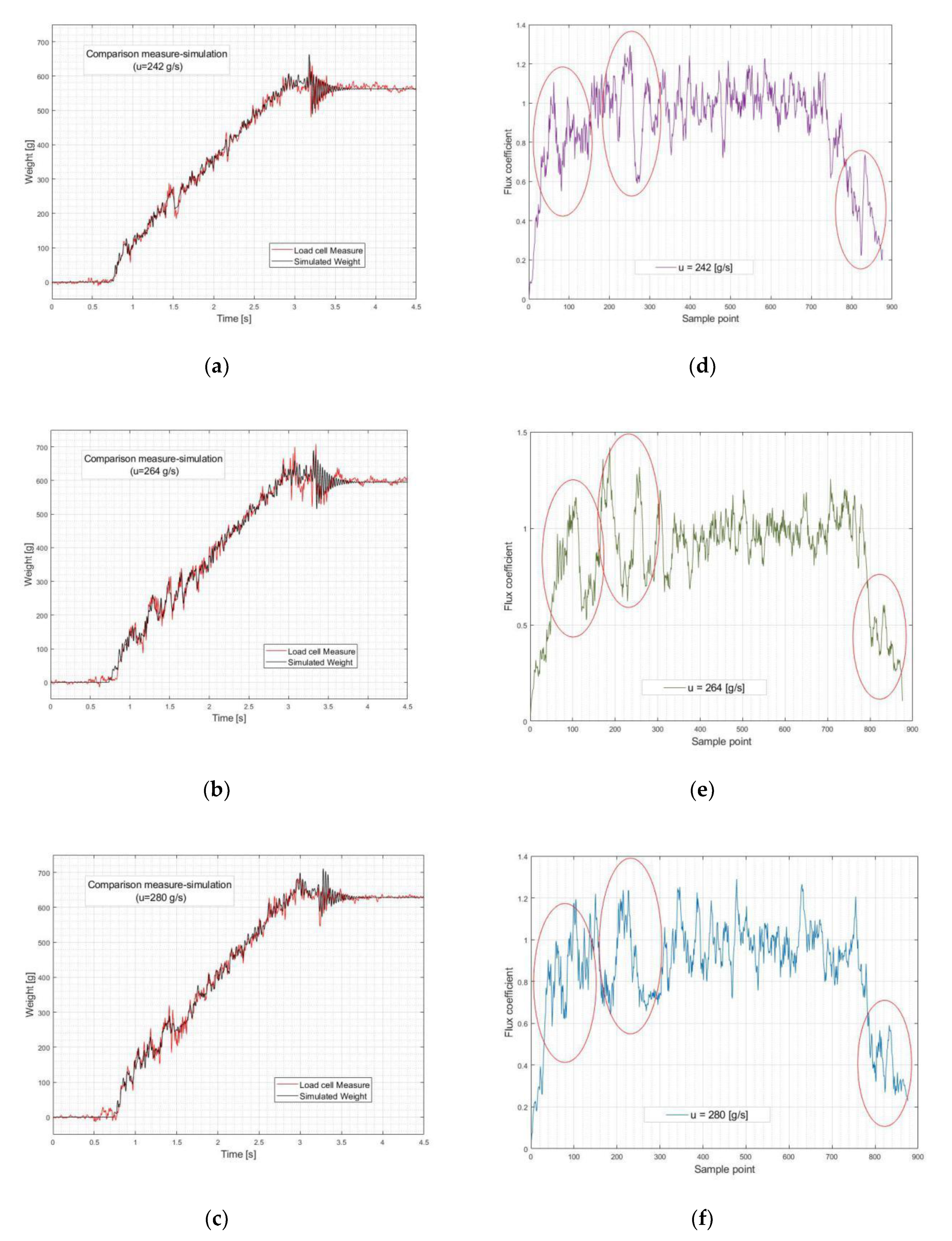
3.2. Model-Based Analysis of the Vibrations

The model presented in Section 3.1 proved to be useful for a better understanding and evaluation of the physical phenomena that characterize the filling process. The tests performed on the machine revealed that the vibration at the end of the filling cannot be explained by only considering the external forces described in Section 3.1. It was deduced that an impulsive force is generated in the machine (with very high probability caused by the spool of the by-pass valve) and this force was introduced in the model.

The approach followed in the model-based analysis consists of two phases:

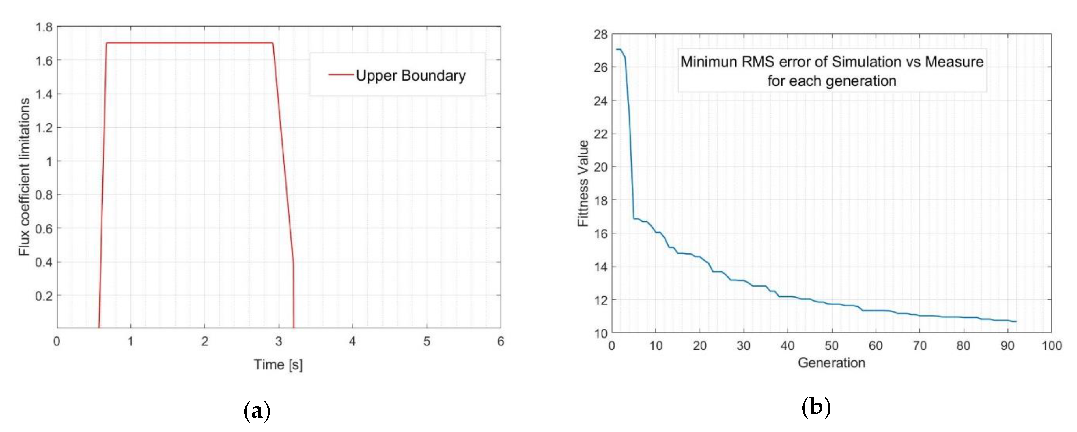
• Phase 1: Identification of the four parameters k, r, Impact force amplitude, Impact force duration, considering a trapezoidal theoretical mass flow pattern;
• Phase 2: Identification of the mass flow rate in the filling with the parameters identified in phase 1.

The motivation for this double identification derives from the fact that, with a theoretical trend of the mass flow, even by varying the characteristics of the trapezoidal trend, it is not possible to reproduce all the vibratory phenomena that are detected by the experimental measures.

The parameters’ identification was based on an optimization procedure, with the use of a genetic algorithm (GA), where λ = (λ₁, λ₂, …, λ_n) denotes the set of characters for each individual. The population of each generation is formed by m individuals and selection, mutation, cross-over rules are applied to obtain the evolution or the population over the generations. The objective function in both of the phases is the root mean square value of the error between the measured weight and the simulated one (RMS_error). In the estimation of the RMS_error, the measured weight is smoothed with a moving average filter. For phase 1, n is equal to four. For phase 2, a point by point mass flow trend during the filling phase was considered, therefore considering a time step dt and a duration of the filling T_f, the number of characters for each individual is n = T_f/dt. The parametric identification problem consists in establishing the set of values λ* = (λ₁*, λ₂*, …, λ_n*), which minimizes the RMS_error objective function, that is:

$${\lambda }^{*} | RMS\_error\left({\lambda }^{*}\right)=min\left(RMS\_error\left(\lambda \right)\right)$$

(9)

In both of the cases, it is a non-constrained optimization problem, with an objective function that is non-differentiable, highly nonlinear, and not well suited for standard optimization algorithms. For this reason, we have chosen a genetic algorithm [16,17]. The GA MATLAB solver, combined with the ODE solver, was used for the identification process. For each individual of a generation, the objective function is evaluated after the numerical solution of the second order differential equation (Equation (9)). The procedure is reiterated several times defining a succession of populations whose best individuals are closer and closer to the optimum (non-divergence of the method is guaranteed by reinserting the best member of previous generation in every new created population). The simulated evolution will stop when a pre-defined goodness target is attained, or when the function to be optimized no longer meets substantial increments. For the flux identification of phase 2, the point by point identification is characterized by a very jagged trend of the mass flow, therefore the vector of the parameters obtained from the genetic algorithm before being used in the model is filtered with a moving average filter with a 10-points window.

Table 1. Main characteristics and parameters assumed for the genetic algorithm used.

Main Characteristics	Parameters
Simulated generations	92
Population’s individuals (m)	200
Characters for individual—Phase 1 (n)	4
Characters for individual—Phase 2 (n)	876
Optimization Problem Type	Non-linear
Cross-over function	Arithmetic
Cross-over fraction	0.8
Mutation Function	Gaussian
Migration Fraction	0.1

reports the main characteristics and parameters assumed for the genetic algorithm used. For the characters of individuals to be identified by the GA, upper and lower boundaries are defined. The lower boundary is set to zero for all of the characters and both of the phases. From the preliminary tests of phase 1, we identified a reasonable maximum value of the parameters; the GA identifies the value of the multiplying factor of the maximum value and therefore the upper limit for all four parameters is one. For phase two, the GA identifies the multiplying coefficient of the nominal value of the flux. Figure 11a depicts the upper boundary limitation of the a-dimensional coefficient for the flux. Figure 11b reports the trend of the objective function value for the best individual of the population in subsequent generations for phase 2. For phase 1, a similar trend was obtained, but the convergence RMS_error value was higher. In all of the identifications carried out, the convergence of the algorithm was obtained after a number of generations of the order of 100. The model-based analysis was performed for the tests on the sixteen stations machine, with three different mean values of the μ(t) mass flow rate. Let u denote the mean value of μ(t); the considered values of u are: 242 [g/s], 264 [g/s] and 280 [g/s]. The identified values of the parameters (k, r, Impact force amplitude, Impact force duration) in phase one were the same for the three different u values: this confirms the reliability of model and method.

Figure 12a–c shows the comparison between the measured (red) and simulated (black) weight in the three considered cases, after the identification of the parameters (phase 1) and flow (phase 2). Figure 12d–f reports the identified flux coefficients for the three cases.

From the analysis of the comparison between measures and simulations, some deductions emerged. As previously stated, an impulsive force is generated when the bypass valve is closed; in different tests the same intensity and duration of this impulsive force has been identified. This allows us to affirm that it represents a characteristic mechanical behavior of the valve and therefore leads to a thorough study of the operation and structure of the valve, considering that the vibration that is induced significantly affects the weighing process. The measurement, in fact, can be considered reliable only when this vibration re-enters within a pre-fixed tolerance band.

From the trend of the mass flow identified in different tests, with different test conditions, it can be observed that there are significant and repeating variations in the initial and final stages of filling. This irregularity in the flow could be determined by the behavior of the valve as well.

4. Conclusions

The experimental tests led to some deductions on the vibrations in the load cell response of automatic weight fillers. The viscosity of the dispensed liquid affects the “noise” of the signal. In fact, water generates a dirtier signal than oil. The parameters that affect the duration and frequency of end-of-fill oscillations are: tank filling level, delivered mass and tap/bottle-free liquid surface distance. In addition, the increase in the tank filling level reduces the oscillation time of the signal, but does not affect the excited frequencies; the end-of-fill oscillation time is directly proportional to the delivered mass, and the impact of the liquid queue, related to the tap/bottle-free liquid surface distance, heavily conditions the signal trend and therefore the reading time. The local vibration modes of the cell/plate system are not responsible for the most consistent vibration recorded by the cell: the vibration is rigid and vertical. From the model-based analysis, it emerged that a source of vibration is related to the flow dynamics. Another source is not internal to the system, but it is due to the valve that manages the opening and closing of the tap. The impact of the spool at the end of the stroke excites the system, generating important oscillations in the cell signal. For those systems where the replacement of the on-off type pneumatic valve with a proportional one is permitted, the latter problem could be solved upstream. In contrast, for the existing machines, this could not be possible. In such cases, the problem may be compensated in two ways: with the application of “intelligent” filters to clean up the signal, or by developing a mathematical model useful to compensate for the most significant vibrations. The implemented model, moreover, makes it possible to indirectly derive the flow rate trend in those systems, like the examined one, in which a direct measurement of the flow is not possible, and to deduce any unwanted system behaviour for condition monitoring purposes.

References

1. Pietrzak, P.; Meller, M.; Niedźwiecki, M. Dynamic mass measurement in checkweighers using a discrete time-variant low-pass filter. Mech. Syst. Signal Process. 2014, 48, 67–76. [Google Scholar] [CrossRef]
2. Jafaripanah, M.; Al-Hashimi, B.; White, N.M. Application of Analog Adaptive Filters for Dynamic Sensor Compensation. IEEE Trans. Instrum. Meas. 2005, 54, 245–251. [Google Scholar] [CrossRef]
3. International Recommendation. OIML R51-1 Automatic Catchweighing Instruments. Part1: Metrological and Technical Requirements—Tests; International Organization of Legal Metrology: Paris, Framce, 2006. [Google Scholar]
4. Sarnecki, R.; Wiśniewski, W.; Ślusarski, W.; Wiłkojć, P. Traceable Calibration of Automatic Weighing Instruments Operating in Dynamic Mode; EDP Sciences: Les Ulis Cedex, France, 2018; Volume 182, p. 02005. [Google Scholar]
5. Stranzinger, S.; Faulhammer, E.; Scheibelhofer, O.; Calzolari, V.; Biserni, S.; Paudel, A.; Khinast, J. Study of a low-dose capsule filling process by dynamic and static tests for advanced process understanding. Int. J. Pharm. 2018, 540, 22–30. [Google Scholar] [CrossRef] [PubMed]
6. Llusa, M.; Faulhammer, E.; Biserni, S.; Calzolari, V.; Lawrence, S.; Bresciani, M.; Khinast, J. The effect of capsule-filling machine vibrations on average fill weight. Int. J. Pharm. 2013, 454, 381–387. [Google Scholar] [CrossRef] [PubMed]
7. Tiboni, M.; Roberto, B.; Carlo, R.; Faglia, R.; Adamini, R.; Amici, C. Study of the Vibrations in a Rotary Weight Filling Machine. In Proceedings of the 2019 23rd International Conference on Mechatronics Technology (ICMT), Salerno, Italy, 23–26 October 2019; pp. 1–6. [Google Scholar]
8. Wasif, H.; Fahimi, F.; Brown, D.; Axel-Berg, L.; Fahimi, F.; Brown, D. Application of multi-fuzzy system for condition monitoring of liquid filling machines. In Proceedings of the 2012 IEEE International Conference on Industrial Technology, Athens, Greece, 19–21 March 2012; pp. 906–912. [Google Scholar]
9. Tiboni, M.; Incerti, G.; Remino, C.; Lancini, M. Comparison of Signal Processing Techniques for Condition Monitoring Based on Artificial Neural Networks. In Applied Condition Monitoring; Fernandez Del Rincon, A., Viadero Rueda, F., Chaari, F., Zimroz, R., Haddar, M., Eds.; Springer: Cham, Switzerland, 2019; Volume 15, pp. 179–188. [Google Scholar]
10. Tiboni, M.; Remino, C. Ondition monitoring of a mechanical indexing system with artificial neural networks. In Proceedings of the WCCM 2017—1st World Congress on Condition Monitoring 2017, London, UK, 13–16 June 2017. [Google Scholar]
11. Pietrzak, P. Fast filtration method for static automatic catchweighing instruments using a non-stationary filter. Metrol. Meas. Syst. 2009, 16, 669–676. [Google Scholar]
12. Hernandez, W. Improving the response of a load cell by usingo ptimal filtering recursive least-squares(RLS) lattice algorithm to perform adaptive filtering. Sensors 2006, 6, 697–711. [Google Scholar] [CrossRef] [Green Version]
13. Boschetti, G.; Caracciolo, R.; Richiedei, D.; Trevisani, A. Model-based dynamic compensation of load cell response in weighing machines affected by environmental vibrations. Mech. Syst. Signal Process. 2013, 34, 116–130. [Google Scholar] [CrossRef]
14. Aguilera, J.; Engel, R.; Wendt, G. Dynamic-weighing liquid flow calibration system—Realization of a model-based concept. In Proceedings of the 14th FLOMEKO 2007, Johannesburg, South Africa, 18–21 September 2007. [Google Scholar]
15. Aguilera, J. Dynamic weighing calibration method for liquid flowmeters—A new approach. In Proceedings of the 56th International Scientific Colloquium, Ilmenau, Germany, 12–16 September 2011. [Google Scholar]
16. Gen, M.; Lin, L. Genetic Algorithms. In Wiley Encyclopedia of Computer Science and Engineering; Wah, B.W., Ed.; John Wiley & Sons, Inc.: Hoboken, NJ, USA, 2008. [Google Scholar] [CrossRef]
17. Michalewicz, Z.; Janikow, C.Z. Genetic algorithms for numerical optimization. Stat. Comput. 1991, 1, 75–91. [Google Scholar] [CrossRef]
Figure 1. (a) Detail of the main carousel of a weight filler. (b) Details of a station: fluid dispenser and bottle holder plate.
Electronics 09 00995 g001
Figure 2. Schematic representation of the filling phases and related acceleration (light-blue) and weight signals (yellow) behaviors. (a) Tare weight measurement; (b) Filling; (c) Final weighing; (d) Zero condition reset.
Electronics 09 00995 g002
Figure 3. Accelerometers setup: (a) first test campaign on the test-bench (two three-axial and two mono-axial); (b) second test campaign on the weight filler (one mono-axial).
Electronics 09 00995 g003
Figure 4. (a) Load cell signal (red), filtered load cell signal (black) and acceleration signal (blue) for a test on the test-bench. (b) PSD of the signals.
Electronics 09 00995 g004
Figure 5. (a) PSD of the load cell signal; (b) FRF of the acceleration in the three directions; (c) FRF of the load cell and of the vertical acceleration signals.
Electronics 09 00995 g005
Figure 6. (a) Signal of the load cell of a filling system with water as fluid. (b) Signal of the load cell of a filling system with oil as fluid.
Electronics 09 00995 g006
Figure 7. System parameters varied during the tests ( h and   h 1 ). (a) Parameters highlighted on a weight filler station. (b) Schematic representation of a station.
Electronics 09 00995 g007
Figure 8. (a) Estimation of Δt time ( t 2 t 1 ) (b) Influence of the container geometry and of the tank filling level on time Δt; (c) Influence of the delivered mass on time Δt.
Electronics 09 00995 g008
Figure 9. (a) Influence of the container mass on the PSD of the load cell signal. (b) Influence of the tank filling level on the PSD of the load cell signal; (c) Influence of the distance DS (between the dispenser and the plate).
Electronics 09 00995 g009
Figure 10. (a) Mass-spring-damping model and adopted notation. (b) Schematic free body diagram of mass m(t).
Electronics 09 00995 g010
Figure 11. (a) Upper boundary limitation of the a-dimensional coefficient for the flux; (b) Trend of the objective function value for the best individual of the population in subsequent generations.
Electronics 09 00995 g011
Figure 12. Comparison between the measured (red) and simulated (black) weight with (a) u = 242 (g/s), (b) u = 242 (g/s), (c) u = 242 (g/s); Flux coefficient identified with (d) u = 242 (g/s), (e) u = 242 (g/s), (f) u = 242 (g/s).
Electronics 09 00995 g012