SAPTM: Towards High-Throughput Per-Flow Traffic Measurement with a Systolic Array-Like Architecture on FPGA

Abstract

Per-flow traffic measurement has emerged as a critical but challenging task in data centers in recent years in the face of massive network traffic. Many approximate methods have been proposed to resolve the existing resource-accuracy trade-off in per-flow traffic measurement, one of which is the sketch-based method. However, sketches are affected by their high computational cost and low throughput; moreover, their measurement accuracy is hard to guarantee under the conditions of changing network bandwidth or flow size distribution. Recently, FPGAplatforms have been widely deployed in data centers, as they demonstrate a good fit for high-speed network processing. In this work, we aim to address the problem of per-flow traffic measurement from a hardware architecture perspective. We thus design SAPTM, a pipelined systolic array-like architecture for high-throughput per-flow traffic measurement on FPGA. We adopt memory-friendly D-left hashing in the design of SAPTM, which guarantees high space utilization during flow insertion and eviction, successfully addressing the challenge of tracking a high-speed data stream under limited memory resources on FPGA. Evaluations on the Xilinx VCU118 platform with real-world benchmarks demonstrate that SAPTM possesses high space utilization. Comparisons with state-of-the-art sketch-based solutions show that SAPTM outperforms comparison methods in terms of throughput by a factor of 14.1x–70.5x without any accuracy loss.

1. Introduction

Globally speaking, IP traffic has experienced dramatic growth in recent years. By 2022, the amount of monthly IP traffic will reach 50 GB per capital, representing an increase of about 3.1× relative to 2017 figures (16 GB) [1]. Per-flow traffic measurement, which involves counting the number of packets for each active network flow during a certain measurement period, has long been a key problem in various network applications, including traffic monitoring, load balancing, capacity planning, etc. Achieving per-flow traffic measurement high speed and error-free has become more and more challenging in recent years in the face of massive network traffic. For example, thousands of current flows can appear in a very short period of time (e.g., 5 ms [2]) in today’s data center. However, there is still an increasing need to track the size of all flows (flow size, i.e., the number of packets in a network flow) at all times, especially in data centers [3]. In addition, modern data center networks have scaled up to 100 Gbps or even higher speeds; consequently, measuring network traffic at line rate remains a challenge.

Recently, mainstream approaches to per-flow traffic measurement have centered around sketch-based solutions [4], which utilize ’sketches’, i.e., compact data structures to record or summarize traffic statistics. The main defect of the sketch approach is that the measurement accuracy is not stable, meaning that their accuracy could be influenced by a number of factors, including network bandwidth and flow size distribution [5]. In fact, this approach only guarantees an error bound. In addition, according to [6], most state-of-the-art sketches suffer from a high cost CPU overhead and low throughput (typically < 5 Gbps), which is far lower than the high throughput that a state-of-the-art Ethernet switch can provide (e.g., Barefoot Tofino${}^{\mathrm{TM}}$2 can process packets at 6.4 Tbps).

FPGA platforms have been widely deployed in contemporary data centers, as they can provide substantial performance and power improvements for many popular applications including machine learning, gene sequencing, and 5G wireless. In addition, some presently deployed FPGA platforms are armed with a 100+ GbE networking capacity, representing good high-speed network processing ability. Therefore, we can observe the trend that FPGAs have become attractive options for high-speed network processing; this is based on the fact that the reconfigurability of FPGA fits well with the concept of SDN (Software Defined Network). When deploying sketches on FPGA, the mismatch between the throughput and processing speed of the host and FPGA will lower the utilization of FPGA, causing a bottleneck in network traffic measurement performance.

Accordingly, this work focuses on measuring the frequency of all flows on FPGA with high throughput. To ease the burden of the collector, we do not consider adopting any sketch methods; instead, we opt to record each flow independently. The associated challenges exit are two-fold: 1. firstly, how to insert flows efficiently given the limited on-chip memory available on FPGAs; 2. secondly, how to evict flows in a timely fashion to make room for new flows in the face of large amounts of flows coming at the line rate.

Overall, this paper makes the following major contributions:

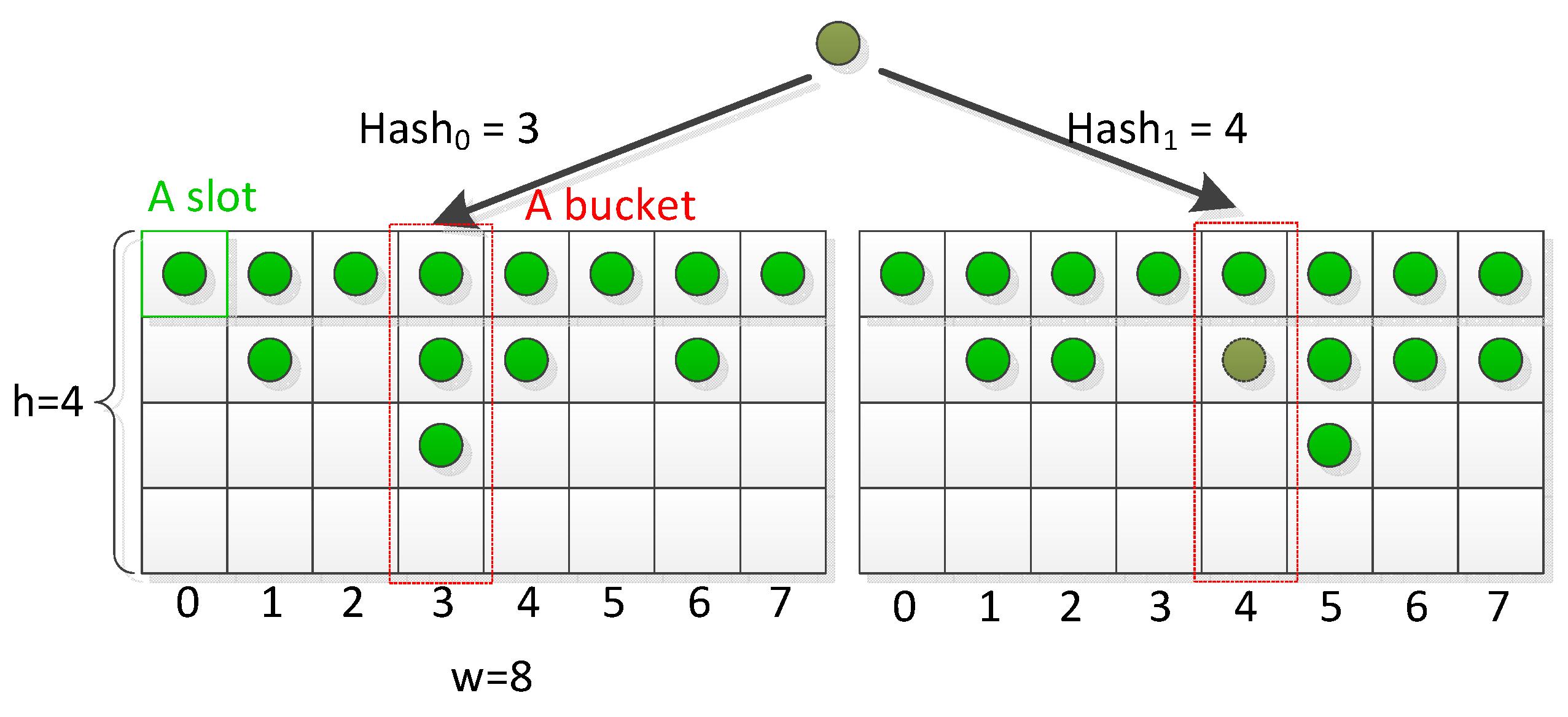
• We propose a systolic array-like multi-stage architecture, named SAPTM, for per-flow traffic measurement purposes. SAPTM enables it to exploit the hardware parallelism of FPGA to pipeline the measurement of flow traffic. Our method also utilizes D-left hashing to improve space utilization, which enables it to trace a large number of flows with only a small storage budget.
• We propose efficient architectural design and working mechanisms for flow insertion and eviction. This approach guarantees that active network flows (flows are extremely large (in total number of packets)) are maintained while mice flows (short flows) with small size are periodically removed from FPGA to the host.
• We prototype SAPTM on the Xilinx VCU118 platform. Evaluations using real-world traces demonstrate that SAPTM can outperform state-of-the-art sketch-based solutions by a factor of 14.1x–70.5x in terms of throughput.

2. Background

2.1. Approaches to Traffic Measurement

Due to the tension between the huge scale of network traffic and the resource limitations of the measurement platform, most existing approaches to traffic measurement are approximate. It can therefore be summarized that there are three main kinds of measurement methods: sampling (e.g., NetFlow [7]), counter-based (e.g., top-k counting) [6,8,9] and sketch-based [5,6,10,11,12] approaches. Sketch-based and counter-based methods are widely used for network traffic measurement. Generally speaking, sketches are mainly used for estimating the sizes of network flows; they keep an approximate count for all flows, while counter-based methods only keep tracking of top-k frequent flows. State-of-the-art sketches have gained success in per-flow traffic measurement. However, most of them introduce high computational cost for CPU to recover the flow sizes. For example, Sketch learn [11] has to calculate tens of thousands of possibilities when estimating the size of a single flow. Moreover, all sketches are not error-free, and their measurement accuracy may be affected by packet rate or flow size distribution [5].

2.2. Measurement Data Structures

2.2.1. Sketch

Representative examples include Count-Min sketch [13] (sketch-based), hashpipe [9] (top-k counting), Cuckoo hashing [14], and D-left hashing [15,16]. CM sketch adopts a kind of “collision embracing” strategy that a sketch count may be written by multiple times, while hashpipe tends to remove an “old” flowkey to make room for the new flowkey when hash collisions occur. Different from CM and Hashpipe, Cuckoo and D-left hashing look for an empty position when hash conflicts occur, rather than removing an “old” flowkey. In other words, Cuckoo and D-left hashing assign a position for each new flow when there is an empty location available.

2.2.2. Hash Table

Most of researches consider a counter-sharing strategy, i.e., all sketch counters may be used to store the statistic of multiple flowkeys. Examples can be found in FlowRadar (Bloom filter), CM sketch, Elastic sketch, etc. The main defect of using this kind of data structure is to determine the size of a given flow, we have to remove the impact of other flows since they also contribute to the data statistic, resulting in measurement error. In addition, the measure accuracy may be determined by some facts such as the size of the sketch counters and the distribution of flows.

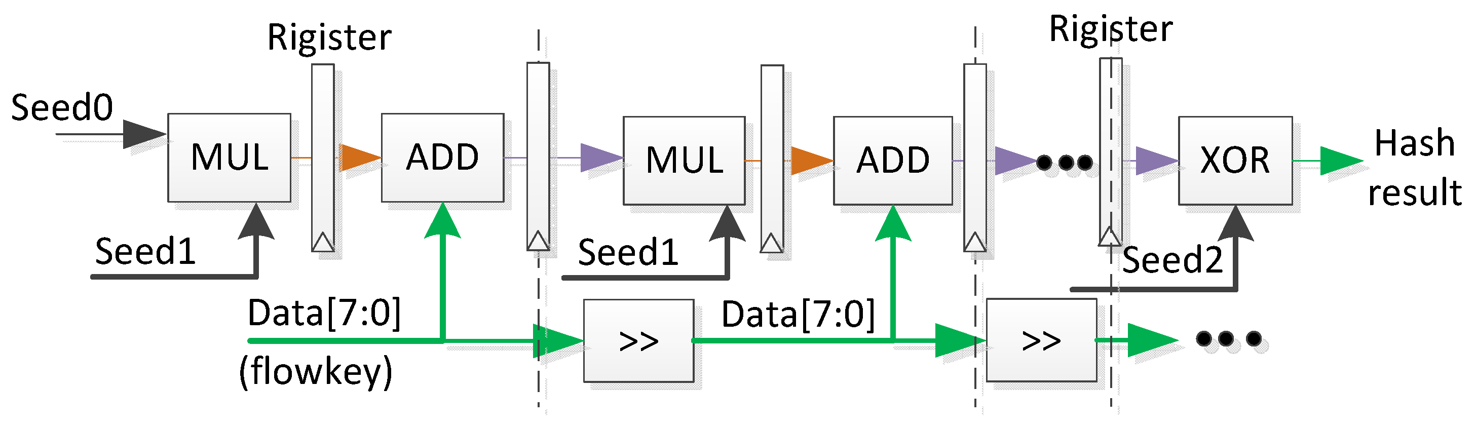
2.3. Memory-Friendly Hash Algorithms

It is vital to improve the utilization of memory in use when measuring a great number of flows on a platform with limited storage. There are some memory-friendly hash methods that can achieve high space utilization when measuring a high number of flows such as D-left hashing. Here, we take D-left hashing as an example. As shown in Figure 1, the hash table is split into d equal sections (or sub-tables, typically $d=2$); moreover, each section contains w buckets, each with h slots ($d\times w\times h$ slots in total). D-left hashing computes d hash functions on the input data to select a hash bucket, then stores the data in the bucket with fewer items in it, using a fixed arbitration scheme (select the left bucket which corresponding to the lower bucket index) if there is a tie. In this way, the workloads of all buckets tend to be balanced, thus facilitating efficient space utilization. Cuckoo hashing adopts a similar but more complex idea: it requires changing the position of old data to make room for a new one when hash collisions occur. In some cases, multiple steps may be required to insert the new data. Obviously, both D-left hashing and Cuckoo hashing will struggle when there are few empty buckets left.

Since Cuckoo has an uncertain number of steps during the insertion, it is infeasible to implement it on FPGA. In this work, we focus on adopting D-left hashing in our design, aiming to reduce the memory requirement of our design by improve the memory utilization.

3. Architectural Design and Implementation

We follow the following principles in designing SAPTM:

• First, SAPTM should be able to exploit the architectural parallelism of FPGA devices. Since FPGA can provide formidable parallel processing capacity, SAPTM should be able to make good use of the characteristics of FPGA, thereby allowing it to efficiently accelerate the procedure of per-flow traffic measurement.
• Second, SAPTM should be able to accurately process all packets at high speed. More specifically, our design goal is to fulfill the line rate requirement of contemporary high speed networks (over 100 Gbps network bandwidth), which puts forward higher requests to the throughput of SAPTM.

3.1. Architecture Overview

Figure 2 depicts the architecture of SAPTM. It can be seen that the key components of SAPTM include the NIC module, Packet Header Parser/Deparser (PHP/PHD), Adaptive Flowkey Dropper (AFD), Hash Array, and the pipelined stages. The NIC module is responsible for reading packets from the high-speed network. Fed by the NIC module, and PHP undertakes the task of extracting flowkeys from the input packets. Note that each flow is identified by a flowkey, which can be defined by any combination of packet fields, for example, 5-tuples (i.e., source/destination IPs, source/destination ports, and protocol). In contrast, PHD functions by re-packaging flowkeys and their corresponding counters and then seeding packets to an NIC module. In addition, Hash Arrays comprising d hash units are used to perform hash computations in parallel.

The pipelined stages are the kernel components of SAPTM and are used to perform the traffic measurement task. All stages except for Stage1 have an identical structure. Different from other stages, Stage1 integrates several critical function units that other stages do not have, such as the Flowkey Tracking Table (FTT), Comparator, and Workload Registers (all of these are marked by red solid boxes). More importantly, all stages are organized in the form of a 1D systolic array-like architecture. On the one hand, data (i.e., flowkeys, hash results, and sketch counters) are only delivered in adjacent stages. On the other hand, the procedures of flowkey insertion/eviction (performed in each stage) and data delivery between stages are performed in parallel.

In addition, the Workload Registers are globally shared by all stages. The main functionality of all stages include flowkey insertion (i.e., recording the flowkeys and their sizes on local counters) and flowkey eviction (i.e., removing the statistics of flowkeys from the current stage and uploading them for analysis). Multiple data paths are designed in these stages to record the flowkeys or deliver the flowkeys as well as the hash results, to the next stages. We split the entire D-left hashing table into all stages equally, and use a group of Workload Register files designed to provide global workload information for all stages. There are several advantages of using SAPTM for per-flow traffic measurement: (1) multiple flowkeys can be processed in different stages simultaneously, which contributes to a strong parallel processing capacity; (2) both intra- and inter-stage processing is carried out in pipeline form, which leverages the throughput of packet processing. Compared to the one-stage counterpart (i.e., using a single stage with a large hash table), our pipelined multi-stage solution ensures a higher hardware utilization and throughput in processing packets.

Workflow of SAPTM

When a network packet is fetched from the high speed network interface, the NIC module first buffers the packet’s header into Packet Header FIFO. Note that the payload of the packet is dropped in the NIC. Then SAPTM reads the extracted flowkey from the Packet Parser. After that, the extracted flowkey passes through the hash units inside the Hash Array to generate multiple hash results in parallel. SAPTM fetches the flowkey and the corresponding hash results once they are available, it then determines the destination stage of the flowkey in the first stage (i.e., Stage1). In each stage, each flowkey has two possible datapaths: namely, being recorded in the current stage or being passed to the next stage (Section 3.3). In addition, old flowkeys will be periodically evicted from the resided slot based on their activeness as well as the load condition of the hash tables (Section 3.4). At the end of each measurement epoch (a time period for traffic measurement, call epoch), the statistics recorded in all stages will be evicted and delivered into the preceding stages (if they exist) via the Inter-data Queue. The Packet Deparser will gather the flowkey and its counter, and send them back to NIC after packaging them back into network packets (the counter of the flowkey is served as the payload of the packet). Note that a host CPU which serves as a collector is responsible for gathering the packets.

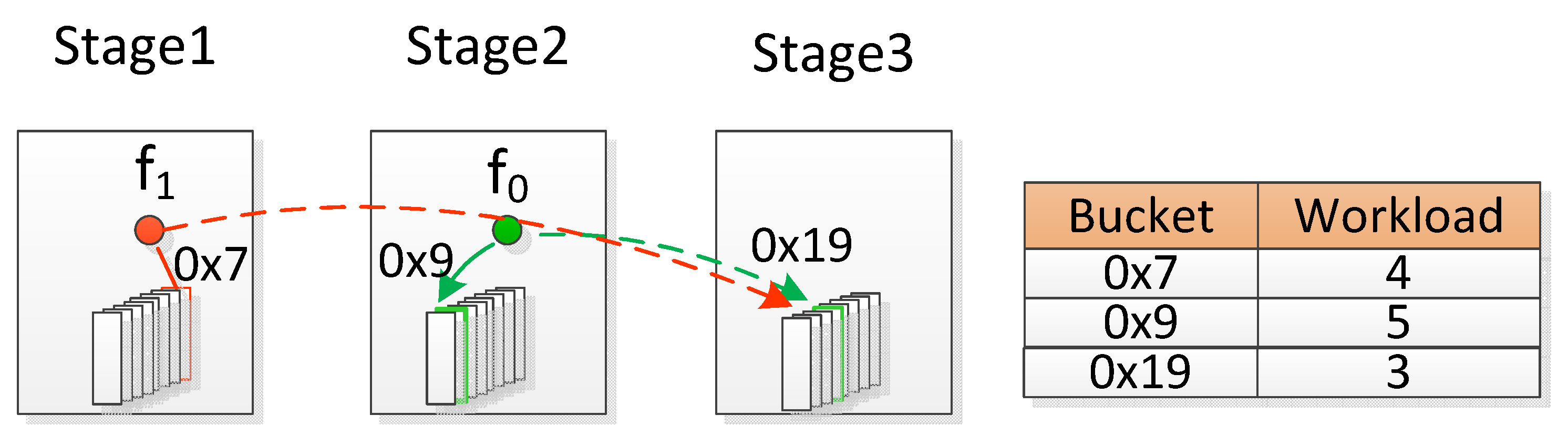
3.2. Hash Table Deployment among Pipelined Stages

How can the d hash sub-tables be efficiently deployed among the $N_s$ stages? We believe that a good hash table deployment should make flowkeys hashed to each stage equally. In this way, we can avoid the unbalanced situation in which some stages are busy processing flowkeys while other stages are hungry for flowkeys. To address this issue, we propose the following solution: namely, dividing each hash sub-table (ST) into $N_s$ parts vertically (i.e., different slots for each bucket are placed in the same stage). In this way, we can obtain $d\times N_s$ sub-subtables (SST) of equal size $\frac{h\times w}{N_s}$. We then assign the $i_{th}$ sub-subtables (i.e., $SS{T}_{ij}$, $1\le i\le d,1\le j\le N_s$) of $S{T}_1\sim S{T}_d$ to the $i_{th}$ stage. As a result, each stage contains a re-organized hash table of size $\frac{d\times w}{N_s}$. To facilitate better understanding, we present a simple example in which $d=3$ in Figure 3. Since each stage is assigned with a hash table of equal size, each flowkey has an equal possibility to be hashed into any stage, contributing to the balanced workload between stages.

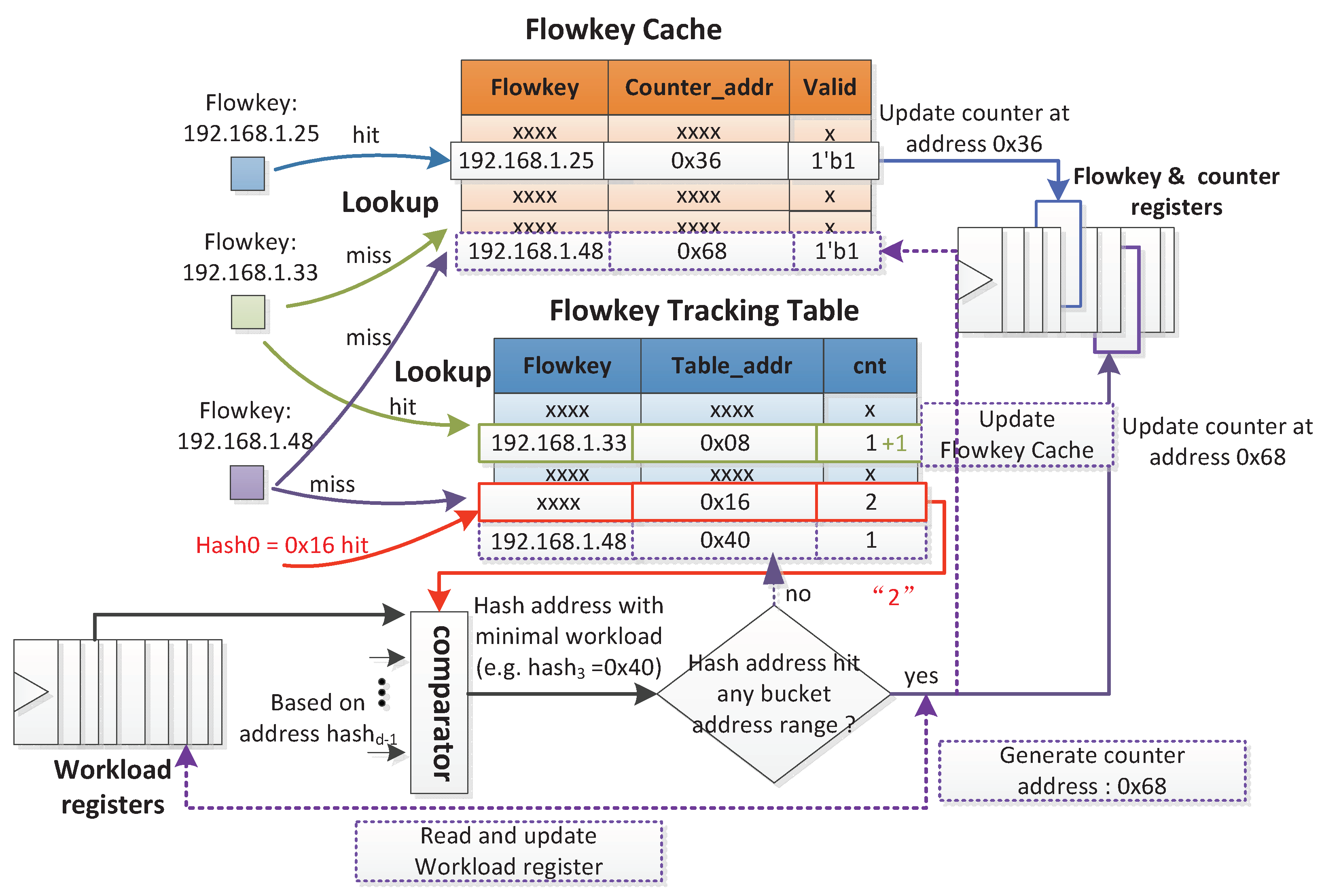
3.3. Flowkey Insertion

Figure 4 shows the procedure of flowkey insertion in Stage1. Note that Stage1 has the most complex datapaths compared with other stages. Here, we only detail the data paths in Stage1:

Data path 1: an incoming flowkey will trigger the issue of a query to FC. If the flowkey matches a cache line (see the example flowkey of 192.168.1.25), the counter address previously stored in the cache line will be fetched, after which a “read-update-write” operation is carried out to the counter indexed by the address. At this point, the flowkey is successfully inserted into the current stage, and no information needs to be delivered to the next stage. If the flowkey does not match any cache line in FC, we regard the flowkey as belonging to a new flow for this stage (it may belong to an old flow recorded in other stages or a brand new flow for all stages), then it will be sent to data path 2.

Data path 2: the flowkey triggers the further issue of a query to FTT (by comparing the exact value of the flowkey). Once a match is found, the “cnt” filed of the matched table entry will be updated by adding one (see the example flowkey of 192.168.1.33). After that, the flowkey and hash results will be directly delivered to the next stage. If the flowkey fails to match any table entry in FTT, meaning that the flowkey belongs to a new flow for all stages, then it would go to data path 3.

Data path 3: when the flowkey appears in this data path, it is required to detect whether there exist data hazards in stages. Therefore, d independent lookup queries are issued to Flowkey Tracking Table (using the d hash results). If there exists a query that successfully responded, the ’cnt’ file of the matched table entries will be read and sent to the Comparator. In the meantime, Comparator also read the workloads of buckets according to the d hash results. In this way, the Comparator identifies the bucket address with the lowest workload among the d candidate buckets (i.e., $BAdd{r}_l=0x40$ in the example), which is used to determine which stage that this flowkey should be recorded in. For the case in which $BAddd{r}_l$ matches the assigned address space of the current stage, we need to find a new location to store the flowkey and assign a new counter for it. In the meantime we add a new cache line containing its information in FC, and update the corresponding Workload Register. However, if it is determined to be recorded in the latter stage, it is required to add a new table entry in FTT (shown in purple dotted box) to record the flowkey (along with $BAdd{r}_l$). Finally, in a similar way to data path 2, the flowkey is sent to the next stage along with the hash results.

Distinguishing between new and old flows. A critical issue during flowkey insertion involves determining whether an incoming flowkey belongs to an old or new flow. FlowRadar [3] utilized a Bloom filter [17] to distinguish between new and old flows. However, a Bloom filter requires multiple memory accesses for each flowkey, which is not hardware-friendly as this could introduce significant memory access overhead. Moreover, motivated by the classical concept of a Cache, we introduce a data structure named Flowkey Cache (FC), which can help us detect whether a flowkey is old or new by storing the recently processed flowkeys as well as their corresponding counter addresses. If a flowkey matches the content in a cache line of FC, we would regard the flowkey as belonging to an old flow that has been recorded in the current stage. Otherwise we would regard it as a new flowkey. Compared to the Bloom filter, using FC requires only one memory access to determine whether the incoming flowkey belongs to an old flow, which contributes to a lower memory access overhead. However, it is unfeasible to design an FC of large size due to the memory limit of FPGA. However, reducing the size of $FC$ could have a negative impact on its hit ratio. To address this issue, we introduce a notation, namely average packet distance (APD), which is defined as the average distance between every two adjacent packets in a flow. We present a simple example to explain APD in Figure 5 for better understanding. We carry out experiments on evaluating the APD of flows from CAIDA [18] (2018). As depicted in Figure 6, elephant flows tend to have a much smaller APD than most of the mice flows. This observation motivates us in that if we store the mice flows in the FC, the hit ratio of FC will be much higher. Therefore, we opt to keep as many as the active elephant (with a low APD) flows in the FC. We can record the activeness of all flows stored in $FC$, and remove them if they are not matched by any flowkeys during a time threshold. Note that the time threshold is set according to the general value of APD of large flows.

Data hazard during flowkey insertion. As shown in Figure 7, consider a situation in which $f_0$ is still being processed in Stage2, and it is decided that it will be hashed to the bucket in Stage3, given that the workload of the bucket at 0x9 is higher than that of the bucket at 0x19. However, one of the two hash values of the next flowkey $f_1$ (0x7 and 0x19) is identical to that of $f_0$ (i.e., 0x19). At this point, since the workload of the bucket at address 0x19 has not yet been updated by $f_0$, an incorrect decision may be made to pass $f_1$ to Stage3 given that the workload at 0x19 is lower than 0x7. This issue is very similar to that of the data hazard in the CPU pipeline. To address this issue, we design a data structure, named Flowkey Tracking Table (FTT) in Stage1, used to record the statistics of the flowkeys that have passed through but have not been recorded in Stage1. Each table entry includes three fields: flowkey, target bucket address (i.e., hash result), and record time. When a flowkey matches a table entry of FTT, the ’record time’ field will be read to help compare the workloads of the hashed buckets of the flowkey. In this way, the current comparison result will be accurate. Note that once a flowkey recorded in FTT is successfully recorded in a stage, the stage will inform Stage2 intermediately to remove the flowkey from FTT.

3.4. Flowkey Eviction

As shown in Figure 8, flowkey eviction—i.e., removing old flows to make room for new flows in the hash table, is a critical problem in per-flow traffic measurement. We have investigated some classical methods to address this issue. NetFlow [7] stores the time at which a flow is last seen and periodically scans the entire hash table to check the inactive time of each flow. If a flow is inactive for a period that exceeds the inactive timeout, NetFlow removes the flow and exports its counts. The main drawback of this method is that it is infeasible to scan the entire hash table, which could result in untenable memory access overhead. In addition, it is difficult to determine a suitable inactive timeout. Some sketch-based methods tend to keep elephant flows in the hash table while removing the mice flows. However, the principles to distinguish between elephant and mice flows may vary substantially between traces. If all flows are comparable in size, this method may decrease in effectiveness. Accordingly, in this paper, we propose a simple but efficient flow eviction strategy: namely, taking the workload condition of buckets as well as the activeness of flows into consideration.

We propose a conservative removal strategy to avoid removing active elephant flows. To be more specific, we start to remove flowkeys only if (1) there are buckets in which workloads reach the alert threshold; (2) the candidate flowkeys in the buckets that meet the first condition are further determined to be inactive, i.e., they are not accessed within a certain time limit. Only if both of these conditions are met, will we start the flowkey eviction procedure. It should be noted here that the candidate flowkeys that meet condition (1) are randomly selected; while this may result in the mistaken selection of active flowkeys in the next few cycles, the second condition will prevent this mistake. Since we do not track the activeness of all flows in the hash table, the candidate flowkeys are randomly selected. These flowkeys are then stored into a data structure named Candidate Eviction Table (CET). Note that the Candidate Eviction Table is designed to be placed in each stage; in this way each stage can remove flowkeys independently. We continue to track the activeness of the candidate flowkeys. If the slot corresponding to the flowkey is accessed during the activeness threshold, we remove the flowkey, and update the workload of the corresponding bucket simultaneously; otherwise, all flowkeys in CET will be removed once the activeness threshold is reached. Figure 4 depicts the procedure of flowkey eviction in detail. It is important to note that the evicted flows as well as their counters are sent back to the collector (i.e., the host CPU) rather than being dropped, which ensures the high accuracy of our design.

3.5. Implementation Details

Figure 9 shows the architecture of a hash unit. From the above, it can be seen that this architecture comprises multipliers, adders, and some simple logics (i.e., shift and xor units). In addition, Seed0∼Seed2 are pre-populated constant data. Moreover, to ensure that the data paths in the hash unit are fully pipelined, we place registers between each pair of computation units.

The functionality of Flowkey Cache, Flowkey Tracking Table, and Candidate Eviction Table is similar to ternary content addressable memory (TCAM). To simplify the design, we use Flip-Flops (FFs) on FPGA to implement these modules. However, implementing $FC$ would demand tens of thousands of FFs if we store the entire flowkeys (about 104 bit), which could fail to meet the time closure. To address this issue, we only store some partial bits of each flowkey in $FC$. Once a flowkey matches a cache line in $FC$, it is required to fetch the entire flowkey from the storage for flowkeys according to the address recorded in the matched cache line. Since the sizes of $FTT$ and $CET$ are much smaller than $FC$, we directly store the entire flowkeys in both of them.

4. Performance Modeling

In this section, we introduce a performance model to help us evaluate the performance of SAPTM. The parameters used in this section are listed in

Table 1. Parameter definitions.

Definitions	Parameters
Number of stages	$N_s$
Latency of hash computation	$L_{ha}$
Latency of Flow Cache lookup	$L_{lfc}$
Latency of writing Flow Cache	$L_{wfc}$
Latency of writing Flowkey Tracking Table	$L_{wft}$
Latency of updating Flowkey Tracking Table	$L_{uft}$
Latency of Flowkey Tracking Table lookup	$L_{lft}$
Latency of updating flowkey counter	$L_{ufr}$
Latency of writing storage for flowkey and counter	$L_{wfr}$
Latency of updating Workload Registers	$L_{uwr}$
Latency of Comparator	$L_{cp}$
Latency of writing Data queue	$L_{dq}$

.

We first evaluate the throughput of the Stage1 in SAPTM. Note that the performance of SAPTM is determined by that of Stage1. From Section 3.3, we know that Data path 3 in Stage1 is the most critical path, given that the data paths in the other stages are simpler. For a flowkey that enters this data path, it must have ➀ failed the FC lookup, ➁ failed the FTT lookup (by comparing flowkey), and ➂ compared the workloads of corresponding hash addresses. This is alternatively followed by two groups of operations: group1 involves ➃ writing FC, ➄ writing storage for flowkeys and counters, and ➅ updating Workload Registers; group 2 involves ➆ writing FTT and ➇ writing Data Queue. It is important to note that the following flowkey can not enter Stage0 until ➃ or ➄ has been completed. Since FC, FTT are implemented using independent memory units, ➀ and ➁ can thus be done in parallel; however, the operations in group1 and group2 can be done until ➂ finishes. As a result, the latency (in cycles) of Data path 3 in Stage1 can be calculated as follows:

$$\begin{array}{cc}{L}_{s1\_dp3}=\hfill & max\{L_{lfc},d\times L_{lft}\}+L_{cp}\hfill \\ \hfill & +max\{L_{wfc},L_{wfr},L_{uwl},L_{wft},L_{dq}\}.\hfill \end{array}$$

(1)

Moreover, the throughput (the total traffic volume processed per second, which can be transformed into a packet rate if the average packet size in known) of SAPTM can be determined as follows:

$$T{P}_{SAPTM}=Siz{e}_{flowkey}\ast \frac{L_{s1\_dp3}}{freq},$$

(2)

where $Siz{e}_{flowkey}$ denotes the size of each flowkey (in MB), and $freq$ (in MHz) is the working frequency of $SAPTM$.

We further model the processing latency of flowkeys processed in other stages, which can be calculated as follows:

$$L_{sn\_dp}=L_{hash}+L_{lfc}+max\{L_{ufr},L_{wfc},L_{wfr},L_{dq}\},$$

(3)

where $L_{hash}$ denotes the latency of the Hash Array. We will next formulate the average processing latency of a single flowkey, as follows:

$$\begin{array}{cc}{L}_{avg}\hfill & =L_{hash}+L_{s1\_dp3}+\frac{1}{N_s}\times L_{s{n}_{d}p}\times (1+2+...+(N_s-1))\hfill \\ \hfill & =L_{hash}+L_{s1\_dp3}+\frac{N_s\ast L_{sn\_dp}}{2}.\hfill \end{array}$$

(4)

In Equation (4), we assume that each flowkey can be recorded in any stage with equal probability (i.e., $\frac{1}{N_s}$). The following can be concluded from Equations (1) and (4): namely, that (i) a small d is beneficial for improving the throughput of SAPTM, and (ii) it seems that a large $N_s$ will have a negative impact on $L_{avg}$. However, given a fixed memory budget, increasing $N_s$ will decrease the memory allocation in each stage; this means that $L_{fc}$ could be reduced accordingly, which is beneficial for improving throughput of $SAPTM$. Therefore, the selection of $N_s$ is critical for the throughput of SAPTM.

5. Evaluations

5.1. Experimental Setup

Benchmarks. The workloads used to test the performance of SAPTM come from a one-hour backbone trace collected in 2018 from CAIDA [18] (location: New York, time: 2018/05/17), and we randomly select a one-minute trace for testing, which contains 26,391,238 packets and 1,361,853 flows. According to our study, there are 2,445,768 times of simultaneous occurrences of multiple packets in the selected trace, and the maximum number of concurrent packets is 14.

Implementation platform. We implement our design on an Xilinx VCU118 FPGA board, which integrates a high-capacity VU9P FPGA and two 64 GB DDR4. The physical host (i.e., the collector) has a six-core Intel Xeon E5-2620 v3 CPU (2.40 Hz) and 128 GB RAM. Note that the host CPU connects to the FPGA platform with the help of an Intel ethernet adapter (XL710-QDA2, 40 GbE NIC).

Software counterpart. To compare the performance of SAPTM with software solution, we carried out experiments on evaluating five state-of-the-art sketch-based solutions, including Deltoid [19], UnivMon [10] (UM), Reversible Sketch [20] (RS), FlowRadar [3] (FR), and SketchVisor [6] (SV). We deploy the selected sketch-based solutions on a testbed composed of three hosts. Similarly, each host is equipped with a 40 GbE NIC. We run the data planes of the sketch-based solutions in one host, and the control plane in the remaining hosts. The control plane functions by periodically collecting the measurement results from multiple hosts and merges them to provide network-wide measurement results, while the data plane mainly performs the measurement tasks and returns the local measurement results to the control plane.

Design parameters. We set a fixed storage budget in SAPTM for all experiments, i.e., $w=4096$, $h=8$, and $d=2$. In addition, the sizes of flowkeys and counters are also fixed to 13 bytes and 4 bytes, respectively.

5.2. Experimental Results

Resource Utilization.

Table 2. Resource utilization.

Resources	${\mathit{N}}_{\mathit{s}}$	BRAMs	DSPs	LUTs	FFs
utilization	4	255 (12%)	68 (1%)	124K (5.7%)	110K (4.6%)
	8	265 (12%)	68 (1%)	127K (5.9%)	138K (5.8%)
	16	285 (13%)	68 (1%)	135K (6.3%)	160K (5.5%)
	32	325 (15%)	68 (1%)	142K (6.6%)	188K (6.8%)
	64	405 (19%)	68 (1%)	150K (6.9%)	202K (8.5%)

reports the resource utilization (placement and routing results) of implementing SAPTM on VU9P with different $N_s$. It can be seen that the overall resource utilization of our design is very low (partly because we use a high-capacity FPGA to implement our design), which contributes to its high working frequency of SAPTM. In addition, SAPTM consumes over 10% of BRAMs (36Kb) as reported, which can be explained by the fact that most of the consumed memory is used to store flowkeys and counters. In addition, it can also be seen that the consumption of $FFs$ (mainly used for implementing $FC$) maintains at a low level as we increase $N_s$ from 4 to 64. This is because we reduce the number of cache lines of $FC$ in each stage along with the increase of $N_s$, for example, we set 256 cache lines in $FC$ for $N_s=4$, while the number of cache lines is reduced to 16 when $N_s=64$. DSPs are only used to implement the hash units, therefore only 1% of the available DSPs are consumed.

Table 3. Actual value of parameters in our implementations.

Parameters	Cycles
$L_{ufc}$, $L_{ufft}$, $L_{wfc}$, $L_{wft}$, $L_{wfr}$, $L_{cp}$, $L_{dq}$	1
$L_{lfc}$, $L_{lft}$	1
$L_{ufr}$, $L_{uwr}$	2

shows the actual value of parameters in our implementations.

Space utilization. To illustrate that SAPTM can maintain good space utilization of D-left hashing, we also implement the D-left hashing algorithm on the host CPU for comparison. Note that the means and variances of the workloads (occupied slots) in all stages are used as the evaluation metrics. In the experiment, we set $N_s=8$, and the numbers of tested packets and flows are 48,579 and 10,000, respectively. It can be seen from Figure 10 that our FPGA implementation can achieve comparable workload means (represented by columns) and variances (represented by lines) to the host CPU, which confirms the effectiveness of our design.

Studies on $N_s$. We conduct experiments to evaluate the performance of SAPTM under different $N_s$, note that we use throughput (Gbps) as the performance metric. In order to increase the performance of SAPTM, we connect the output of the last stage to the first stage, which is beneficial for placement and routing of SAPTM on FPGA. As shown in Figure 11, SAPTM reaches the highest throughput and frequency when $N_s=32$. After that, SAPTM suffers from performance reduction as $N_s$ increases. First, when $N_s<32$, the performance improvement comes from the decrease of the size of $FC$ in each stage. Second, the reason for performance reduction after $N_s=32$ is that all stages (except Stage1) have direct connections to Stage1 for accessing the Workload Registers and updating FTT, thus increasing $N_s$ would introduce long wires, which could lower the working frequency and thus throughput of SAPTM.

Comparisons with state-of-the-art. We compare the performance of SAPTM with five state-of-the-art sketch-based solutions mentioned above. We consider two metrics: (i) CPU overhead (in seconds), i.e., the entire latency for per-flow traffic measurement (including flow recovering), which is measured in the host CPU (control plane); (ii) effective throughput (in Gbps), which can be calculated by Equation (5). We think all solutions (including ours) only process the packet header rather than the entire packet, thus we use effective throughput rather than throughput (as shown in Equation (6)) as the performance metric. Note that the average packet size of the tested trace is 910 bytes, and the size of packet headers is 20 bytes. In our experiments, SAPTM integrates 32 stages, and it is clocked at 358 MHz.

$$EffectiveThroughput=\frac{sizeofpacketheader\times numberofpackets}{processingtime}$$

(5)

$$Thoughput=\frac{averagesizeofpackets\times numberofpackets}{processingtime}$$

(6)

Figure 12 and Figure 13 show the results. It can be seen that SAPTM achieves significant improvement in terms of CPU overhead and throughput over all the sketch-based solutions. More specifically, Figure 13 shows that SAPTM can achieve a performance gain of 14.1x–70.5x (relative to SketchVisor and Detoid, respectively) over the sketch-based solutions, and the average performance improvement over all the tested sketch-based solutions is 32x, demonstrating the effectiveness of our solution. The reasons SAPTM shows higher performance than the selected sketch-based solutions include: (1) by analyzing the breakdown of the CPU overhead in each sketch-based solution, we find that hash computation bottlenecks the performance of some solutions. For example, FlowRadar incurs more than 63% of CPU cycles on hash computations. However, our solution integrates customized logic for accelerating hash computation (see Section 3.5), thereby we can achieve higher performance than the software solutions; (2) in addition, we further observe that some sketch-based solutions perform complex operations on the flows, for example, Deltoid has to update its extra counters to encode flow headers, which is a time consuming procedure. In our solution, SAPTM only performs simpler operations on the flow; (3) moreover, in most of the sketch-based solutions, a sketch counter would be used to record the statistics of multiple flows, therefore the procedure of flow recovering is more complex than ours.

In addition, SAPTM can achieve 100% accuracy in per-flow traffic measurement (which is much higher than the sketch-based solutions) since SAPTM counts for each flow independently, which is different from the sketch-based solutions. In addition, SAPTM would not drop flows but deliver the statistics of all the recorded flows to the host, which ensures the high accuracy of SAPTM. In summary, SAPTM shows a higher throughput and higher accuracy for per-flow traffic measurement than state-of-the-art solutions.

6. Conclusions

This work proposed SAPTM, a novel architecture for per-flow traffic measurement on FPGA. To better utilize the expensive on-chip memory of FPGA, we adopt the classic D-left hashing in SAPTM. Efficient strategies are proposed to improve the space utilization via efficient flow insertion and eviction. It is evident from the experimental results on real-world traces that SAPTM can outperform software counterparts in throughput by a factor of 14.1x–70.5x without any accuracy loss, showing a good prospect for the architecture design for large-scale network traffic measurement in the future.

References

1. Cisco. Cisco Visual Networking Index: Forecast and Trends, 2017–2022 White Paper. 2019. Available online: https://www.cisco.com/c/en/us/solutions/collateral/service-provider/visual-networking-index-vni/white-paper-c11-741490.html (accessed on 27 February 2019).
2. Roy, A.; Zeng, H.; Bagga, J.; Porter, G.; Snoeren, A.C. Inside the social network’s (datacenter) network. In Proceedings of the ACM SIGCOMM Computer Communication Review, London, UK, 17–21 August 2015; Volume 45, pp. 123–137. [Google Scholar]
3. Li, Y.; Miao, R.; Kim, C.; Yu, M. Flowradar: A better netflow for data centers. In Proceedings of the 13th {USENIX} Symposium on Networked Systems Design and Implementation ({NSDI} 16), Santa Clara, CA, USA, 16–18 March 2016; pp. 311–324. [Google Scholar]
4. Yang, T.; Gao, S.; Sun, Z.; Wang, Y.; Shen, Y.; Li, X. Diamond Sketch: Accurate Per-flow Measurement for Big Streaming Data. IEEE Trans. Parallel Distrib. Syst. 2019, 30, 2650–2662. [Google Scholar] [CrossRef]
5. Yang, T.; Jiang, J.; Liu, P.; Huang, Q.; Gong, J.; Zhou, Y.; Miao, R.; Li, X.; Uhlig, S. Elastic sketch: Adaptive and fast network-wide measurements. In Proceedings of the 2018 Conference of the ACM Special Interest Group on Data Communication, Budapest, Hungary, 20–25 August 2018; pp. 561–575. [Google Scholar]
6. Huang, Q.; Jin, X.; Lee, P.P.; Li, R.; Tang, L.; Chen, Y.C.; Zhang, G. Sketchvisor: Robust network measurement for software packet processing. In Proceedings of the Conference of the ACM Special Interest Group on Data Communication, Los Angeles, CA, USA, 21–25 August 2017; pp. 113–126. [Google Scholar]
7. Claise, B. Cisco Systems Netfow Services Export Version. RFC 3954; Cisco: San Jose, CA, USA, 2005. [Google Scholar]
8. Metwally, A.; Agrawal, D.; El Abbadi, A. Efficient computation of frequent and top-k elements in data streams. In Proceedings of the International Conference on Database Theory, Edinburgh, UK, 5–7 January 2005; Springer: Heidelberg, Germnay, 2005; pp. 398–412. [Google Scholar]
9. Sivaraman, V.; Narayana, S.; Rottenstreich, O.; Muthukrishnan, S.; Rexford, J. Smoking out the heavy-hitter flows with hashpipe. arXiv 2016, arXiv:1611.04825. [Google Scholar]
10. Liu, Z.; Manousis, A.; Vorsanger, G.; Sekar, V.; Braverman, V. One sketch to rule them all: Rethinking network flow monitoring with univmon. In Proceedings of the 2016 ACM SIGCOMM Conference, Florianopolis, Brazil, 22–26 August 2016; pp. 101–114. [Google Scholar]
11. Huang, Q.; Lee, P.P.; Bao, Y. Sketchlearn: relieving user burdens in approximate measurement with automated statistical inference. In Proceedings of the 2018 Conference of the ACM Special Interest Group on Data Communication, Budapest, Hungary, 20–25 August 2018; pp. 576–590. [Google Scholar]
12. Tang, L.; Huang, Q.; Lee, P.P. MV-Sketch: A Fast and Compact Invertible Sketch for Heavy Flow Detection in Network Data Streams. In Proceedings of the IEEE INFOCOM 2019-IEEE Conference on Computer Communications, Paris, France, 29 April–2 May 2019; pp. 2026–2034. [Google Scholar]
13. Cormode, G.; Muthukrishnan, S. An improved data stream summary: the count-min sketch and its applications. J. Algorithms 2005, 55, 58–75. [Google Scholar] [CrossRef] [Green Version]
14. Pagh, R.; Rodler, F.F. Cuckoo hashing. J. Algorithms 2004, 51, 122–144. [Google Scholar] [CrossRef]
15. Azar, Y.; Broder, A.Z.; Karlin, A.R.; Upfal, E. Balanced allocations. SIAM J. Comput. 1999, 29, 180–200. [Google Scholar] [CrossRef]
16. Vöcking, B. How asymmetry helps load balancing. J. ACM (JACM) 2003, 50, 568–589. [Google Scholar] [CrossRef]
17. Bloom, B.H. Space/time trade-offs in hash coding with allowable errors. Commun. ACM 1970, 13, 422–426. [Google Scholar] [CrossRef]
18. CAIDA. The CAIDA UCSD Statistical Information for the CAIDA Anonymized Internet Traces. 2018. Available online: http://www.caida.org/data/passive/passive_trace_statistics.xml. (accessed on 27 February 2019).
19. Cormode, G.; Muthukrishnan, S. What’s New: Finding Significant Differences in Network Data Streams. IEEE/ACM Trans. Netw. 2004, 13, 1219–1232. [Google Scholar] [CrossRef]
20. Schweller, R.; Li, Z.; Chen, Y.; Gao, Y.; Gupta, A.; Zhang, Y.; Dinda, P.A.; Kao, M.; Memik, G. Reversible Sketches: Enabling Monitoring and Analysis Over High-Speed Data Streams. IEEE/ACM Trans. Netw. 2007, 15, 1059–1072. [Google Scholar] [CrossRef] [Green Version]
Figure 1. The procedure of D-left hashing.
Electronics 09 01160 g001
Figure 2. Block diagram of SAPTM architecture.
Electronics 09 01160 g002
Figure 3. An illustrated example for table deployment.
Electronics 09 01160 g003
Figure 4. Procedure of flowkey insertion.
Electronics 09 01160 g004
Figure 5. Illustration of packet distances of network flows.
Electronics 09 01160 g005
Figure 6. Evaluation results of package distances of flows in real-world traces.
Electronics 09 01160 g006
Figure 7. Data hazard during flowkey insertion.
Electronics 09 01160 g007
Figure 8. Procedure of flowkey eviction.
Electronics 09 01160 g008
Figure 9. Architecture of a hash unit.
Electronics 09 01160 g009
Figure 10. Comparisons of workload distributions of d-left hashing implemented on CPU and FPGA.
Electronics 09 01160 g010
Figure 11. Throughput and working frequency of SAPTM with different N s .
Electronics 09 01160 g011
Figure 12. Comparison results of SAPTM with sketch-based solutions (CPU overhead).
Electronics 09 01160 g012
Figure 13. Comparison results of SAPTM with sketch-based solutions (effective throughput).
Electronics 09 01160 g013