Abstract
With the enhancement of the sensitivity of gravitational wave (GW) detectors and capabilities of large survey facilities, such as the Vera Rubin Observatory Legacy Survey of Space and Time (LSST) and the 2.5 m Wide Field Survey Telescope (WFST), we now have the potential to detect an increasing number of distant kilonova (KN). However, distinguishing KN from the plethora of detected transients in ongoing and future follow-up surveys presents a significant challenge. In this study, our objective is to establish an efficient classification mechanism tailored for the follow-up survey conducted by WFST, with a specific focus on identifying KN associated with GW. We employ a novel temporal convolutional neural network architecture, trained using simulated multi-band photometry lasting for 3 days by WFST, accompanied by contextual information, i.e., luminosity distance information by GW. By comparison of the choices of contextual information, we can reach 95% precision and 94% recall for our best model. It also performs good validation of photometry data on AT2017gfo and AT2019npv. Furthermore, we investigate the ability of the model to distinguish KN in a GW follow-up survey. We conclude that there is over 80% probability that we can capture true KN in 20 selected candidates among ∼250 detected astrophysical transients that have passed the real–bogus filter and cross-matching.
1. Introduction
The merger of binary neutron stars (BNS) and neutron star-black hole (NSBH) could be the source of thermal emission extended from near-infrared to ultraviolet, which is powered by r-process-generated radioactive decay of heavy elements in the ejecta during the merger, often referred to as kilonova (KN) [1,2,3]. It is believed that kilonovas are typically fainter than supernovas and fast fading within a week [4,5]. Often during this process, a highly relativistic jet along the polar axis could launch short ray bursts (sGRB) lasting for a few seconds [6,7,8]. The interaction of the jet and interstellar medium powers the X-ray afterglow, which is spread within a relatively wide viewing angle [9,10,11,12]. The dawn of multimessenger astronomy associated with gravitational wave (GW), heralded by the detection of a compact binary merger, GW170817, and its electromagnetic (EM) counterparts AT2017gfo and GRB170817A, has ushered in a new era of multimessenger astrophysics [2,3,13,14,15,16,17,18,19,20,21,22,23,24]. With the completion of the thereafter third LIGO/Virgo observing run, O3, and a total of 90 GW candidates identified, GW astrophysics has jumped into a time-domain era [25,26]. In addition, the observation of EM signature has allowed for more accurate inclination and distance measurements of the host galaxy by model fitting and identification. In fact, EM counterparts of GWs are important sources of bright standard sirens to constrain the Hubble constant, e.g., for GW170817, which could shed light on the Hubble tension problem [27,28].
In the span of the O3 run, a total of 56 public alerts were released by LIGO/Virgo through the gamma-ray coordinate network (GCN) notices and circulars1 [25]. While extensive prompt follow-up observations were conducted following low latency public alerts, which yield hundreds to thousands of candidates, no confirmed kilonova was identified [29,30]. The reason for the undesirable outcome is controversial. The fast-fading signature of KN and very limited sky coverage induced by poor localization might be responsible [31,32]. However, poor sky coverage and selection criteria can also affect the data stream, which indicates that a true KN could be rejected by real–bogus classification, astrophysical origin selection, and even KN classification [30].
The ongoing LIGO/Virgo/KAGRA (LVK) fourth observation run, O4, will reach ∼160 Mpc for BNS merger detection, and over are expected to be detected by LVK [33,34]. The sensitivity of the O5 run will extend to ∼330 Mpc detection in the next decade, which implies the potential for discovering a BNS merger will increase by an order of magnitude. [35]. Many efforts are focusing on rapid deployment and optimization of optical follow-up triggered by GW and GRB public alerts [36], e.g., Zwicky Transient Facility2 (ZTF, [29,37]), Dark Energy Camera3 (DECam, [30,38]), Wide Field Survey Telescope4 (WFST, [39,40]) and next generation Vera Rubin Observatory Legacy Survey of Space and Time5 (LSST, [41,42]).
The 2.5 m WFST, installed at Saishiteng Mountain near Lenghu on the Tibetan Plateau, China, will strongly support various science cases, including time-domain astronomy, asteroids and the solar system, the Milky Way and its satellite dwarf galaxies, galaxy formation and cosmology and so on [40]. With a field of view (FoV) of 6.55 , it could cover ∼ within a night with a 5 depth of 22.31, 23.42, 22.95, 22.43, 21.50 mag under 30 s exposure in five bands (), respectively, making it one of the most powerful facilities in the northern sky for discovering GW counterparts [43]. In addition, excellent observation conditions with an average diopter of arcsec and 22.0 V-band background provide potential for high-quality data [44].
It is common to be overwhelmed by the data stream produced by the rapid and deep searching of wide-field instruments. Since it is not sufficient to identify KN solely by photometry, efficient KN classification is still of great significance for maximizing identified KN. Traditionally, the KN photometry classification is based on several criteria, e.g., decay rate, color evolution [29] or model fitting, and it is upgraded to a complete pipeline, e.g., ZTFReST [45]. Another method is employing a machine learning classifier, which was implemented during O3 and is well-designed so far [30]. Stachie et al. [46] adapted the long-term lightcurve RAPID [47] classifier of short-term KN detections. Chatterjee et al. [48] deployed a KN classifier, which uses a similar structure, including GW skymap information. Biswas et al. [49] designed a fast transient classification algorithm, aimed at KN, which is implemented as a module in Fink broker6, a data stream processor software for ZTF and LSST. Sravan et al. [50] proposed a fully machine-directed pipeline for KN discovery, including the optimization of the survey plan to maximize the chance of identifying KN.
Of great importance is the need for a rapid and efficient KN classifier for the WFST target-of-opportunity (ToO) observation. Thus, in this work, we simulate lightcurve data from KN and contaminants detected by WFST with designed capability, air conditions, and strategies. Subsequently, a modified RAPID framework is employed to train and test the performance of our simulated WFST ToO data generated using mock GW skymaps [35].
This paper is organized as follows. Section 2 describes the simulation of training data. We begin with the mock GW skymaps and survey plans that are generated automatically through the ToO pipeline. KN and contaminants are simulated using Monte Carlo simulations, which follow their space and time distribution, i.e., KN is distributed following GW, and contaminants are distributed following their volumetric rate. Then, we implement mock photometry and collect their lightcurves and associated information such as location and line-of-sight probability. The classifier framework and training process are detailed in Section 3. In Section 4, we test the performance on both the dataset and real data and explore the situation in simulated GW follow-up surveys. Finally, we present our conclusions in Section 5.
2. Transients Simulation
Our simulation has three steps: firstly, we randomly choose mock GW events detected by LVK with O4 sensitivity. For each event, many KN and contaminant objects are placed across the sky. Then, we trigger our KN ToO pipeline to deploy mock surveys. Finally, we collect lightcurves given certain survey plans and contextual information for each object. The full dataset is obtained by iterating all select events.
Since the aim of this work is the KN classifier for WFST during O4, the amount of BNS and NSBH events detected so far is not adequate to cover the diversity of skymaps and survey cadences. Petrov et al. [35] simulated GW signals from BBH, BNS, and NSBH mergers and employed a more realistic threshold under O3, O4, and O5 sensitivity. They gave comparable sky localization to O3 and concluded that the sky localization might be even worse during O4, which coincides with recent observations. Therefore, we randomly chose 250 GW events7 from the BNS merger as our mock events that will happen at random in 2024, in which the WFST will be online.
2.1. Survey Simulation
In practical GW observations, an accurate localization of the event plays a pivotal role in triggering ToO observations. To initiate it effectively, it is essential that the observable area for the event aligns with the survey capability of the telescope, ensuring a sufficiently high probability of observing the specific sky region. In our study, we carefully excluded sections of the localization area falling within of the galactic plane and regions with declination for the mock GW skymaps. Additionally, we incorporated the restriction that the airmass should not exceed two to define the observable sky area for each event. Based on the observable area and the probability of observing the sky region, we filtered 250 events, selecting those that meet the following criteria: an observable area is less than 3000 and the probability of observing the 2D sky region is not less than 0.2. Among them, 68 events finally triggered the ToO survey.
Then, we generated survey plans by implementing gwemopt8, which was originally developed by Coughlin et al. [42], serving the purpose of optimizing the EM follow-up search for GW events. During O3, several post-event observation plans were formulated using gwemopt for both individual and joint observations by multiple telescopes (e.g., [29,51,52,53,54]), yielding good performance.
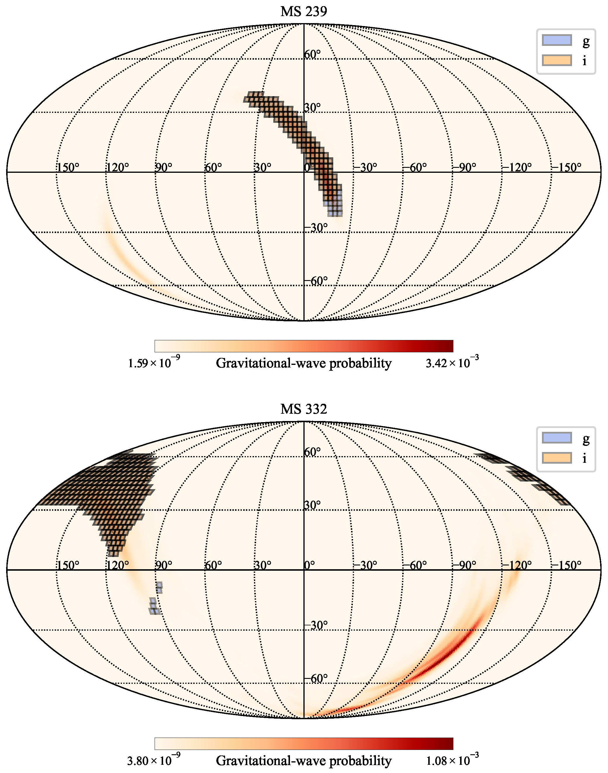
In the process of generating survey plans, gwemopt includes several algorithms within each step: (1) skymap tiling, (2) time allocations, (3) scheduling. Coughlin et al. [42] extensively discussed the efficiency of various combinations of these algorithms, determining that the combination of the (1) MOC algorithm, (2) power-law algorithm, and (3) greedy algorithm yielded the most efficient results. Therefore, we employed this combination of algorithms for our simulations. Specific inputs need to be prepared before running the code, namely the merger event, exposure time, bands, and observation windows. Initially, the merger times for the GW events were randomly distributed from 1 January to 31 December 2024 to match the future operational timeline of O4. The selection of nightly coverage frequencies and bands was based on the observable area of the events and the lunar phase conditions. and bands were prioritized around the new moon and full moon, respectively. We also adjusted our exposure time according to the luminosity distance of the event and the estimated time spent in observation. Currently, we assume an observation window for three days post-merger, during which WFST would repeatedly cover the target area. Upon the completion of the code, it will generate a list containing the corresponding pointings for each exposure, the observation time, and the cumulative probability within the coverage area as output. We show two examples of the GW skymap, MS_239 and MS_332, and the corresponding triggered WFST ToO survey in Figure 1. The tiles in the map are footprints of a one-night survey.

Figure 1.
Examples of mock GW skymap and footprints of WFST ToO observation.
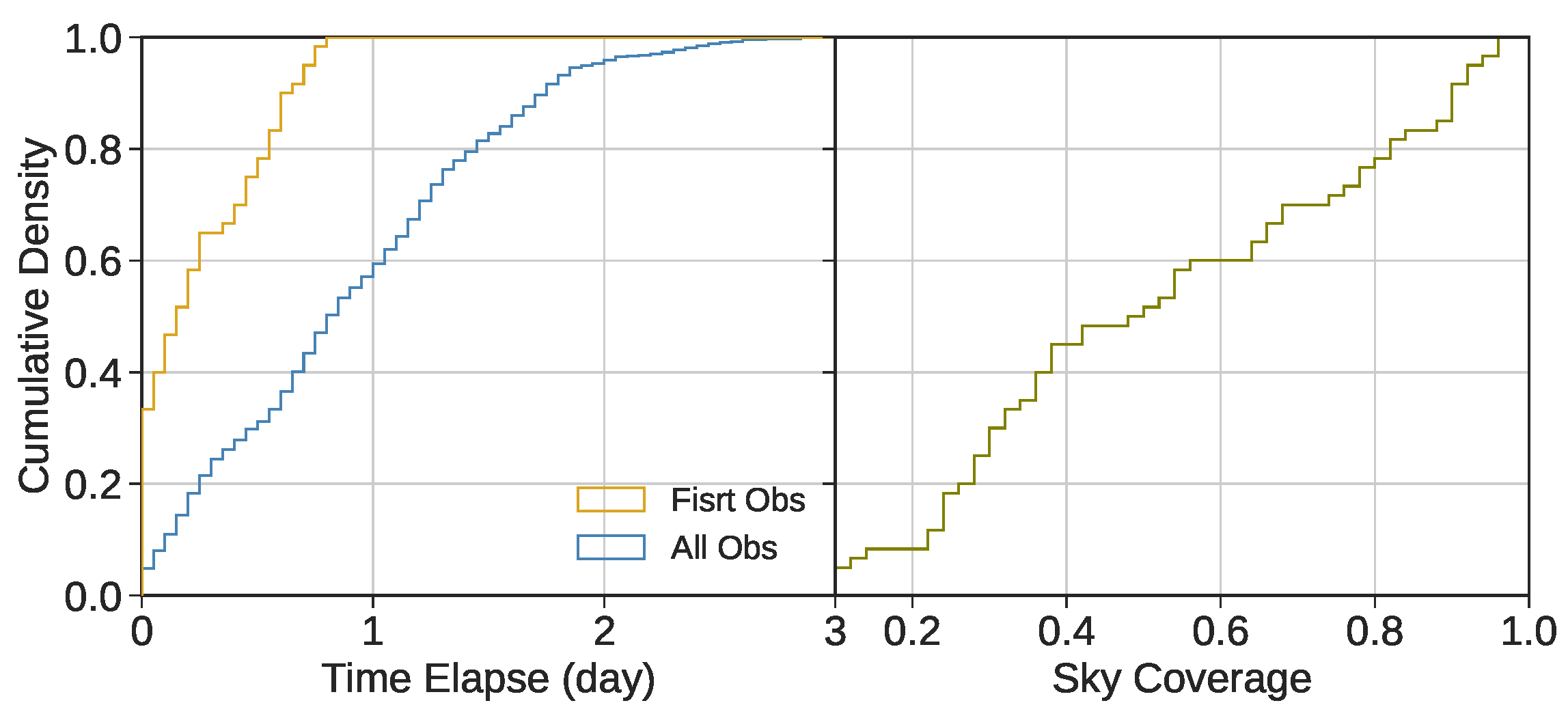
In Figure 2, we show the cumulative density of elapsed time between the follow-up trigger and GW trigger. The first observation time and overall observations are almost uniform within 0.8 days and 2 days, respectively. The sky coverage is also widely distributed between 0.2 and 1, indicating that we have covered as many scenarios as we can.
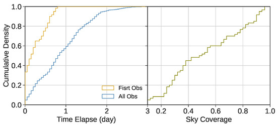
Figure 2.
(Left panel): Cumulative density of time elapsed of the follow-up, first, and all observations. (Right panel): Cumulative density of sky coverage of triggered events by WFST.
2.2. KN Simulation
For the KN simulation, we used two models to generate spectral energy distribution (SED). The first one is a two-component model first presented by Bulla [28,55], in which the spectra of KN were calculated using Monte Carlo radioactive transfer code POSSIS9. The first component, dynamical ejecta, is characterized by mass , which has velocities ranging from 0.08c to 0.3c. There are two compositions that are formed via different channels, in which lanthanide-rich composition is distributed within angle around the equatorial plane, which is formed due to tidal processes and lanthanide-free composition that is otherwise formed by a hydrodynamic interaction. The second component is post-merger wind ejecta, , which is distributed spherically and has relatively lower velocities ranging from 0.025c to 0.08c representing outflow from the accretion disk. To generate SEDs of arbitrary parameters, we construct a surrogate model using a neural network following the method in Ref. [56,57,58]. The ejecta mass and velocity are related to the binary property involving mergers, such as chirp mass, mass ratio, and equation of state (EoS). Many numerical relativity simulations have analyzed the process of merger and KN explosions [59,60,61,62,63,64]. Therefore, it allows us to bridge a connection between the BNS sample and a KN lightcurve sample.
For dynamical ejecta , we used the fitting formula from Coughlin et al. [63], which was extended from Ref. [61,65],
where and represent the mass and compactness of two compact objects, respectively, and fitting constants . represents the exchanging of subscripts. The mass of dynamical ejecta is sensitive to the mass ratio and compactness of neutron stars. We also characterize the fraction of the red component of ejecta presented in Ref. [59,66] that separate lanthanide-rich and -poor components by a threshold ∼0.25 when , whereas for ∼1 because the less massive NS is disrupted by tidal forces that suppress the shock [60,67,68,69]. The fraction of the red component can be written as
with . Using the spherical ejecta density profile assumption in the Bulla model, it is easy to obtain the half-opening angle for lanthanide-rich components.
For post-merger ejecta, we used the following expression to evaluate disk mass [63],
with fitting parameters that include mass ratio dependence and the free parameter given by
where . The best-fit values of free parameters are . is the total mass of BNS, and represents the threshold mass for prompt massive neutron star collapse to a black hole with the expression [28]
where is the maximum stable mass for non-rotating NS, and represents the radii of NS. The disk wind ejecta mass is assumed to be proportional to disk mass with f ranging from 0.1 to 0.5 [70,71,72,73]. In this work, we fixed as the default set. It is noted that explicit density, heating rate and opacity profile, and structured jet are considered in the new version of the POSSIS 2.0 model [74,75].
We also employed another semi-analytical kilonova model presented in Nicholl et al. [66], thereafter MOSFiT KN, which is implemented by the open-source software MOSFiT10. The model is based on the binary property forwarded to SED. They employed a numerical relativity fitting formula to convert binary parameters to ejecta parameters. The ejecta contains three components with different grey opacity, namely blue (), red (), and purple () components. The red and blue components represent dynamical ejecta with higher velocity, and the half opening angle of red ejecta is fixed to . This model also includes the cocoon emission and magnetic enhancement on blue ejecta mass.
Once the KN model is prepared, we can obtain the KN SED sample from a BNS sample and inject their parameters into two KN models. In the standard isolated binary formation channel, a recycled NS is born first and spins up due to the accretion or recycling process. It is accompanied by a non-recycled NS that spins down after birth. The mass of recycled NS follows a two-Gaussian distribution,
with . For non-recycled NS, they are found to follow a uniform distribution within 1.15∼1.42 [76]. Given the mass of the neutron star, we calculated the radius and compactness by sampling the parameterized EoS obtained by Dietrich et al. [28], where the EoS sample was calibrated with constraints of pulsars and multimessenger observation on GW170817. We generated the KN SED sample with a size of ∼ for each KN model.
2.3. Other Transients Simulation
To simulate contaminants, our main focus in this work is on supernovae, one of the most significant types of contaminants following catalog cross-matching. Still, we cannot ignore other important fast transients, e.g., cataclysmic variables (CVs), afterglows, and shock breakouts. They will be included in the complete pipeline with the aid of other selection procedures.
SN Ia. The Type Ia Supernova is thought to be powered by the re-ignition and thermonuclear explosion of carbon–oxygen white dwarfs once they exceed their critical mass [77,78]. It is the most common and numerous contaminant object to KN. To model SN Ia, we used the SED library presented by Hsiao et al. [79]. Apart from classic SN Ia, some subgroups in the SN Ia were identified through decays of observations. SN1991bg-like (SN Ia-91bg) stands out as one of the most important potential contaminants due to their bright, luminous, rest-frame and fast evolution feature, with a lightcurve width of less than 70% average SN Ia [80,81].
SN Ibc. The stripped-envelope supernova explosion, also referred to as Type Ib and Type Ic supernova, characterizes the feature of lacking helium in spectra [82]. The lightcurves of SN Ibc are fainter, redder, and evolve slower, indicating they are sub-dominant sources of contamination. We used the SED template presented in Nugent et al. [83]11 to model SN Ibc, SN Ia, and its subgroups.
SN II. Type II Supernova are explosions of massive stars with mass [84]. They are distinguished from other types by the presence of hydrogen in their spectra. We modeled two subgroups SN IIn and SN IIP using the SED template in Nugent et al. [83].
SLSN-I. Type I Superluminous Supernova is one of the brightest optical transients with peak absolute magnitudes . They are widely distributed in metal-poor dwarf host galaxies, some of which are powered by magnetars with very strong magnetic fields [85]. Their spectra tend to be blue, lack hydrogen features, and brighten rapidly, thus making them the main contaminant in early KN identification [86,87]. To model SED, we employed the extended library of 960 SEDs from the MOSFiT slsn model by Kessler et al. [88].
2.4. Training Set
Given GW skymaps and corresponding survey strategies and transient models described above, we performed a survey simulation implemented by simsurvey12 [89], a software for survey simulation and lightcurve collection [29,89]. The simulated KN for each GW event was sampled randomly based on two KN models in Section 2.2. The explosion time of KN was set the same as the GW event, and its location was produced following the probability density of the GW skymap. For contaminants, we assume a uniform distribution of RA and Dec within the observed field of survey and specific redshift model listed in Table 1.

Table 1.
Summary of transients in the training set.
We randomly looped 60 skymaps and collected their lightcurves and object information, e.g., line-of-sight probability , distance mean and standard deviation derived from GW skymap. It is noted that for supernovas, we truncate the distance with , which is comparable to the detection depth of WFST. Finally, we obtained the data set containing 77,005 objects, the details of which are listed in Table 1. Since we aim to distinguish true KN among many contaminants, we labeled Bulla KN and MOSFiT KN as Kilonova and the rest as Other. Figure 3 shows the normalized distribution of line-of-sight probability, mean, and standard deviation of luminosity distance of transient according to the GW skymap of our dataset per class. One can see that the KN has a tighter distribution of features compared with contaminants because they always happen in the high probability area of the GW skymap. In addition to the lightcurve, these features could also assist us in classifying KN and contaminants.
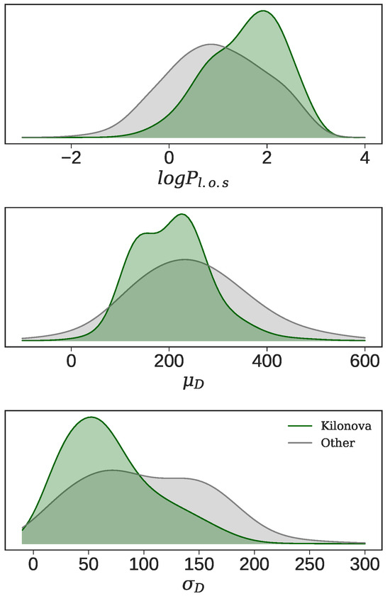
Figure 3.
Distribution of line-of-sight probability, distance mean, and standard deviation of the training set.
3. Binary Classification
We employed temporal convolutional network (TCN) architecture [90], which is implemented in keras13 and RAPID14 for long-term lightcurve classification, revealing good performance. We used a similar architecture to Chatterjee et al. [48], who modified RAPID for binary classification to filter KN.
3.1. TCN Framework
The strength and utility of the TCN architecture in the classification of a time series lie in its ability to promptly update results as new data become available. As introduced by Bai et al. [90] in 2018, the TCN architecture operates on two fundamental principles: (1) The length of the output sequence matches that of the input, and (2) the internal convolutions are causal in nature. Provided with a sequence of data, the TCN outputs a sequence , and the convolutions within the hidden layers of the architecture are designed in such a way that each output, , solely relies on the information within the input sequence , where n ranges from 1 to N. Within this architectural framework, as shown in Figure 4, one can control the extent to which long-term historical information influences the output by making judicious selections of kernel sizes or incorporating dilated layers. Beyond that, one can inject the contextual information as input, which stays unchanged with time. In this work, we consider line-of-sight probability, mean and standard deviation of luminosity distance of transient according to GW skymaps and their combinations. For simulated WFST surveys with the time interval between two photometries ∼1 day, in order to reveal a more precise shape of the lightcurve, we adopt linear interpolation with a time interval 0.5 day within 5 days. Therefore, the dimensions of the input data matrix are , where represents the length of the interpolated time series, the number of passbands, and the amount of contextual information.
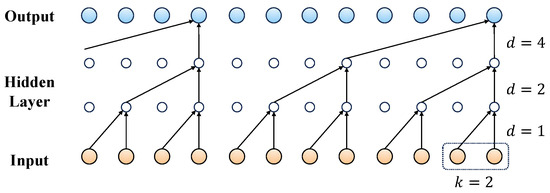
Figure 4.
Framework of TCN with a filter length of 2, and dilation is in hidden layers.
3.2. Training
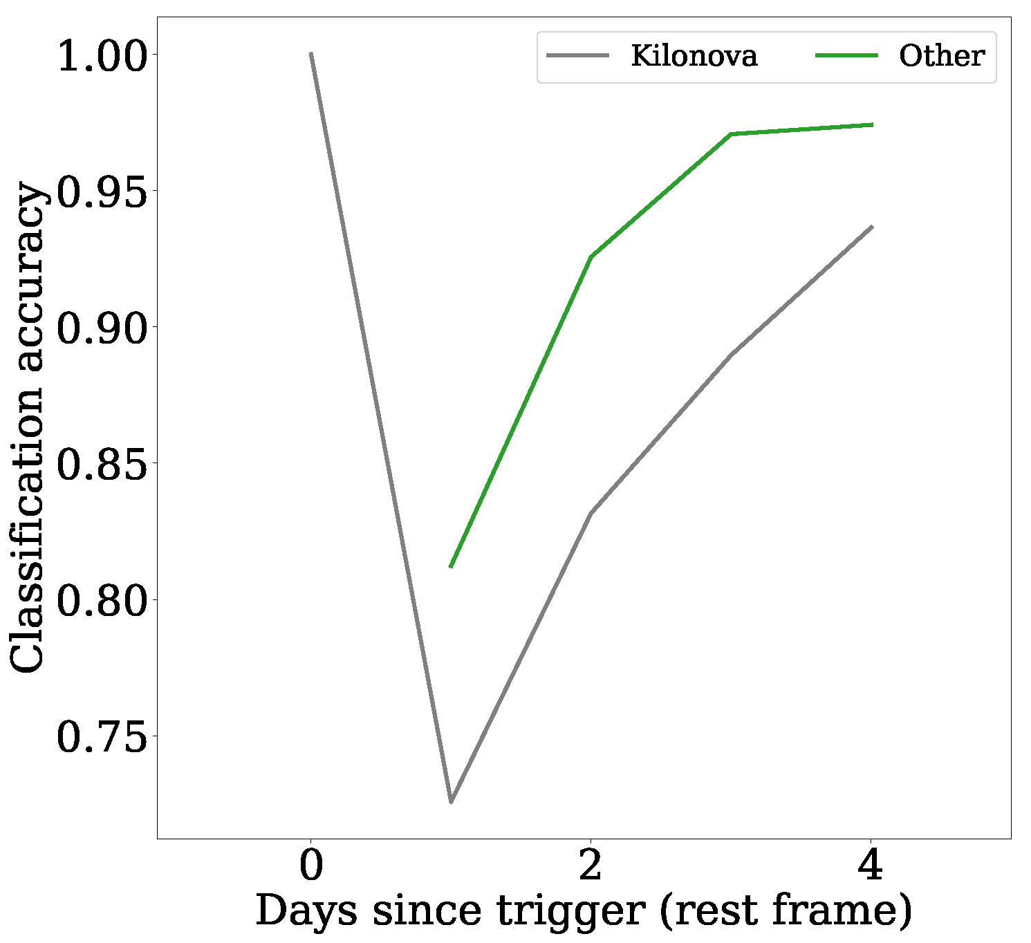
For our purpose of classification for KN in ToO data, which lasts 3 days post-merger, as shown in Figure 2, we used a network of filter length and dilation layers and 2 stacks to deepen the network. We employed categorical cross-entropy as the loss function in conjunction with the Adam optimizer. For the dataset, we partitioned it into a training set comprising 70% of the data and a test set containing the remaining 30%. By testing, we found that loss tends to converge after 50 epochs of training, so we trained models for 50 epochs. Approximately 2–3 h were allocated for training and testing models. Notably, we found that the computational cost for training is comparatively modest, negating the necessity for hardware optimizations, such as GPU acceleration. Figure 5 shows the accuracy per class with time in which at least 3 days of observation yields good accuracy. The classifier tends to predict a high KN score inaccurately in instances where photometry data are lacking, as evidenced by a noticeable decline around day one. However, as more photometry data are processed, the predictions converge more closely toward the actual label.
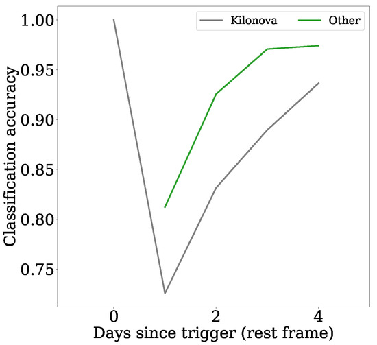
Figure 5.
Accuracy per class with time of the PMD model. Kilonova and Other reached over 98% and 92% accuracy after 3 days since the trigger, respectively, after the inaccurate prediction with a high KN score when lacking photometry data.
As described above, we have three contextual datasets at our disposal to assist in classification: line-of-sight probability (hereafter P), mean, and standard deviation of luminosity distance along the line of sight of transients according to GW (hereafter M and D). To see which data affect the result most and to decide upon the best combination of information used, we consider three combinations of them: MD, PM, and PMD. Our fundamental principle relies on the mean luminosity distance defined by the GW skymap, serving as crucial guidance for the AB magnitude of transients. Therefore, the MD model and PM model lack line-of-sight probability and measurement error of luminosity distance, whereas PMD has full contextual information.
4. Results
4.1. Performance on Dataset
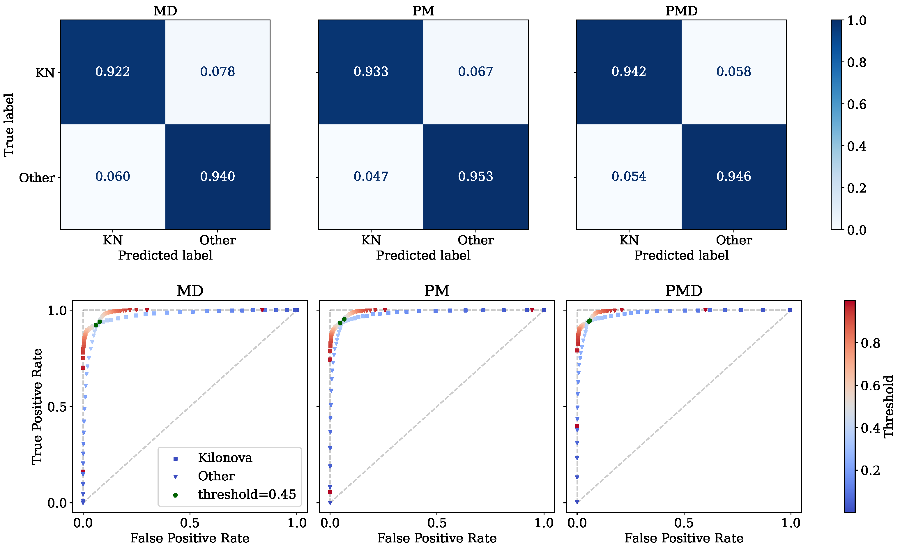
Using the dataset simulated in Section 2 and the TCN framework described in Section 3, we obtain MD, PM, and PMD classification models for WFST targeting KN. Among them, the PMD model reaches an overall accuracy of 98.41%. To test the performance of a classifier, it is natural to employ a confusion matrix to show their capability. In our binary classification issue, the dimensions of the confusion matrix are , with true positives and true negatives residing in diagonal elements, while false positives and false negatives lie in the upper right and lower left elements, respectively. Figure 6 illustrates the confusion matrices for the MD, PM, and PMD models. The matrix values are normalized by the number of true labels, and the KN score is the last KN probability in the sequence of prediction. In the context of prioritizing the detection of KN, a threshold of 0.45 is selected to minimize the potential for false positives. Specifically, we classify a candidate as a KN when the predicted KN probability in the final epoch surpasses this specified threshold. Upon comparing these models, it becomes evident that the MD model exhibits lower efficiency when contrasted with the other two alternatives.
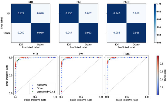
Figure 6.
(Upper panel): Confusion metrics for MD, PM, and PMD models. The values in elements are normalized by the size of true labels per class. (Lower panel): ROC curves with KN and Other are drawn as inverted triangles and squared lines. The color map of the marker denotes the various values of thresholds, and the default value of 0.45 is plotted as green dots.
However, it is obviously unreasonable to use the same threshold for three different models. We estimated the performance of models under various thresholds. In the lower panel of Figure 6, we show the receiver operating characteristic curve (ROC), which illustrates the diagnostic ability of a binary classifier system. The inverted triangle curve and squared curve represent the true positive rate and false positive rate, with threshold ranging from to . The threshold of 0.45 is shown as green dots in each curve. The more powerful the model is, the closer the curve is to the upper left of the coordinate. We summarize their precision and recall with thresholds corresponding to the cross of two curves, yielding 94.151% precision, 94.028% recall for the PM model and 94.830% precision, 94.125% recall for the PMD model. We notice that the PM model and PMD model have comparable capabilities while lacking line-of-sight probability is the most intolerable case.
4.2. Performance on Real Data
To further investigate the performance of the classifier, we employed similar procedures as in Chatterjee et al. [48] to test in unseen data. We considered Swope observations on AT2017gfo [91], originally identified as ‘SSS17a’ by the Swope team at the time of its discovery. It was the only identified KN accompanied by GW so far, with ejecta mass , via the fitting of various KN models [18,24,28]. We used band data to be compatible with our trained model input. Although the optical transmission curves of Swope are different from WFST, we maintain the belief that these disparities in the KN score’s uncertainty will not lead to misleading classification results. Additionally, we also consider a counterpart candidate of GW190814 [92], AT2019npv, which was an SN Ibc but was identified as KN in the early phase by efforts of several teams because it was located in the GW skymap, and the redshift was consistent with the distance information of GW [30,93,94]. We included the first week band observations from DECam as the WFST survey would not exceed 5 days.
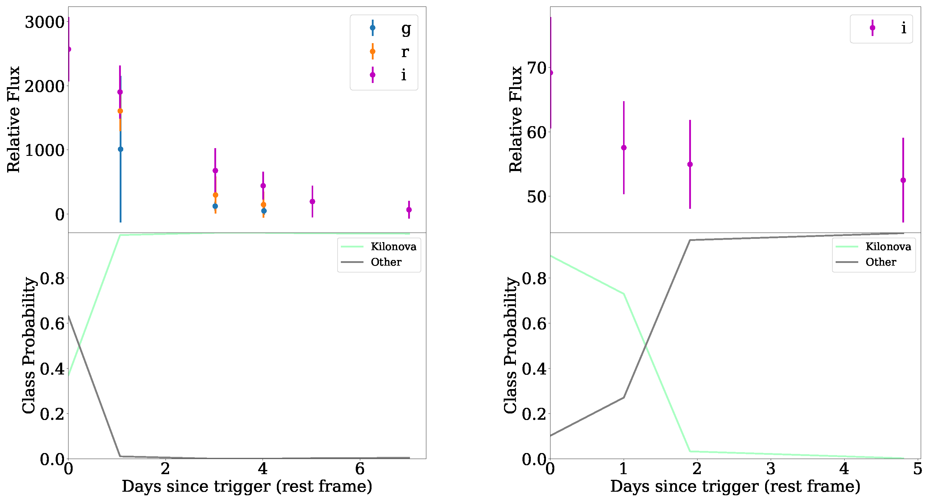
In Figure 7, we implement our PMD model to predict the KN score of AT2017gfo and AT2019npv. We acquired comparable results to Chatterjee et al. [48], in which the confidence KN score is obtained from AT2017gfo and the persuasive primary KN score from AT2019npv at the early phase rather than the definitive contaminants that result from increasing observations.
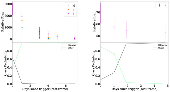
Figure 7.
(Left panel): Prediction of Swope observations on At2017gfo. (Right panel): Prediction of DECam observations on AT2019npv.
4.3. Performance on Mock Survey
We have conducted thorough validation and performance tests of our model as described above. Nevertheless, it remains imperative to assess the model’s efficiency in predicting future survey data, ensuring its practical applicability. To achieve that, we applied simulations with mock surveys, as described in Section 2. In a night survey, the WFST would detect – transients ignoring history activity [40,95]. We assume that approximately a fraction of them can be filtered out by cross-matching or angular offset to their host galaxy. Therefore, we only considered cases of processing less than 300 candidates by classifier. As a comparison, an average of 170 EM candidates were filtered after multi-step machine learning, which includes the real–bogus test, cross-matching, and history exclusion [29]. To simulate candidates processed by classifiers, which have been filtered by the real–bogus test, cross-matching, and history exclusion, we simulated one KN according to the GW skymap and n contaminants with uniform distribution across the sky for each mock survey. Then, we compiled them into a data package labeled as detected candidates. The size of detected candidates is denoted as . We generated five data packages for each skymap for data augmentation, considering the variety of KN models and locations. Overall, we generated 300 data packages, and we ranked KN scores in descending order in each data package, i.e., means the true KN has the highest KN score in detected candidates. According to our pipeline, we will take several selected candidates, the size of them denoted as , for the subsequent spectra follow-up. In our analysis, we chose and . In Figure 8, we show the distribution of ranking of KN with . The top of grey and blue bars represent the maximum and 0.8 quantiles of KN rankings with various , which means over of KN would rank within 20 when does not exceed 290. We also calculated the 0.6 quantile, which remains 1 with any .
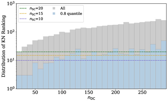
Figure 8.
Distribution of ranking of true KN in a data package with various . The top of grey and blue bars represent the maximum and 0.8 quantiles of KN rankings with various .
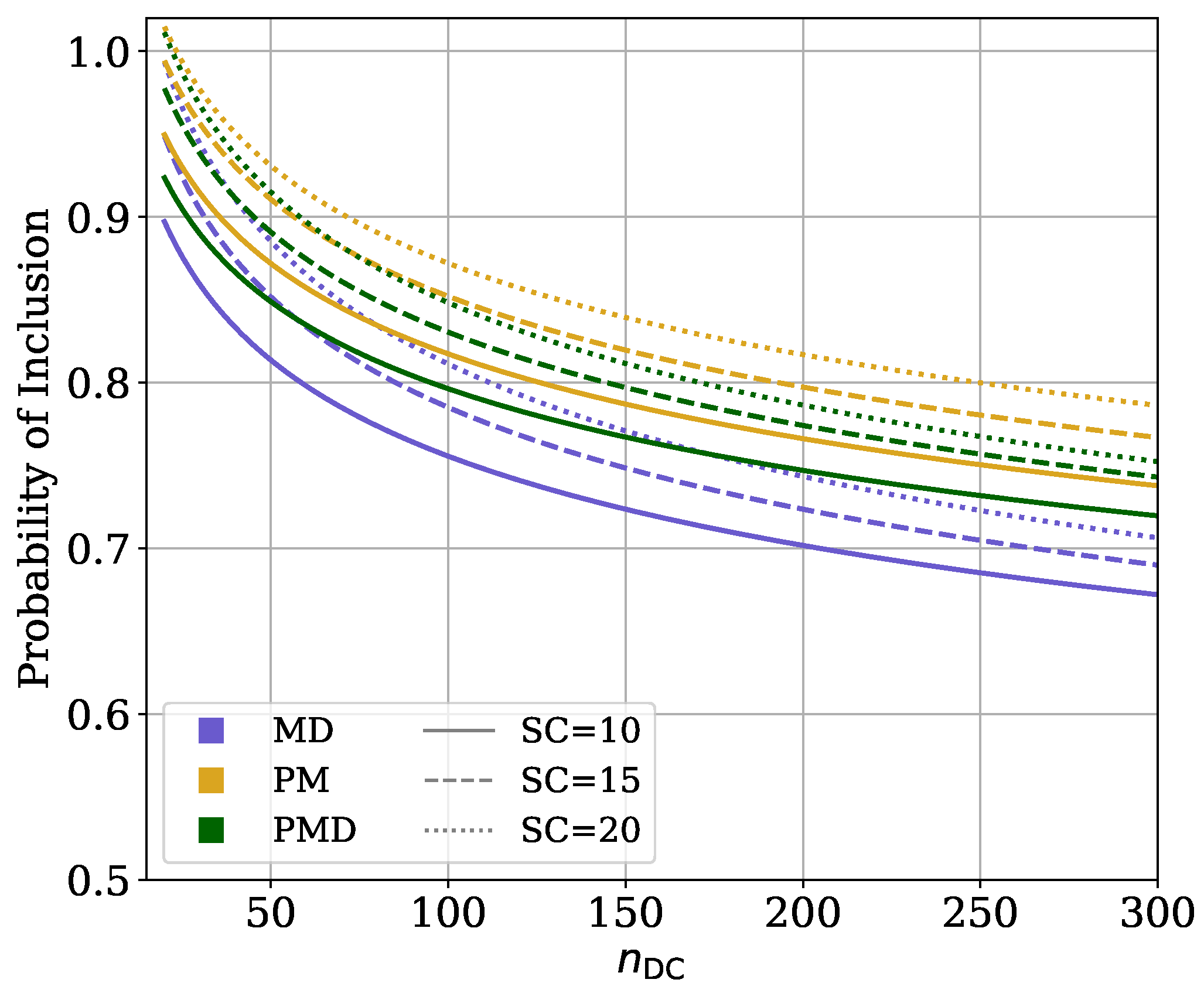
For better clarity, we quantified the fraction of the data package in which the true KN achieved for given as the probability of inclusion. This metric reflects the classifier’s effectiveness in incorporating the true KN among the selected candidates. As expected, the classifier’s performance exhibited a declining trend with an increasing amount of . Notably, we found a good fitting by a power-law function with fitting parameters . The curves are depicted in Figure 9. The results for the MD, PM, and PMD models are illustrated in violet, yellow, and green, respectively, and solid, dashed, and dotted lines corresponding to . The optimal fitted parameters are outlined in Table 2. Leveraging this fitted curve, we can now estimate the likelihood of capturing true KN in future ToO surveys, thus facilitating our choice of . For example, given ∼250 candidates detected and 80% probability of inclusion required, we should characterize .
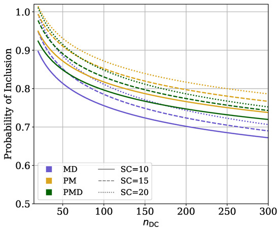
Figure 9.
Best-fit probability of inclusion with for various models. The PM model could reach over 80% probability of inclusion when .
Table 2.
Best fitting parameters for various of three models.
5. Conclusions
In the era of multi-messenger astronomy, especially conducted by LVK and the future 3rd generation Cosmic Explorer (CE; Reitze et al. [96]) and the Einstein Telescope (ET; Maggiore et al. [97]), it will require strongly qualified detectors to be mutually compatible, which necessitates the coordination of numerous facilities to effectively leverage the scientific prospects offered by the upcoming dataset. In light of this, the development of machine learning techniques and integrating physically informed features becomes crucial to streamlining data and minimizing the burden of human screening. The negative outcome during the LIGO/Virgo O3 run indicates that the AT2017gfo-like KN is abnormal, to date presenting substantial difficulty in identifying KN systematically. In the ∼6 months since LIGO/Virgo O4 has been running, many collaborations triggered their ToO observations, e.g., GROWTH15 and MASTER GLOBAL Robotic Net16. To enhance the probability of identifying EM counterparts of GW detections, several brokers have been developed, i.e., KN classifier embedded in Fink broker [49], EI-CIDm, which was based on the RAPID framework [48], ZTFReST [45], AleRCE [98], Lasair [99], SCiMMA17, and a fully automated pipeline for KN discovery [50].
In this work, we have presented a KN binary classifier with a modified RAPID framework. Our approach was inspired by the enhancements detailed in Chatterjee et al. [48], where the fine-tuned neural network exhibited promising performance on simulated ZTF data. We start with the simulation of transients, where we have conducted a mock WFST survey of 60 simulated GW skymaps with O4 sensitivity. The KN is located following the probability distribution of GW skymaps, whereas contaminants are located uniformly across the sky. It is noted that Andreoni et al. [45] found cosmological afterglow to be the dominant contaminant at high galactic latitude within ∼1 yr observations. Furthermore, other contaminant classes, e.g., CVs, afterglows, and shock breakouts, pose potential challenges because only a fraction of them can be filtered by cross-matching with a catalog, implying it would occasionally be a dominant source [49]. Considering that the classifier is designed to operate on processed data ideally filtered through a real–bogus test and the exclusion of variable stars, we have simulated the majority of supernovae, which represent the predominant contaminants following the removal of these sources. Upon these foundations, we have applied three combinations of contextual information, MD, PM, and PMD, revealing comparable performances between the PM and PMD models, while the MD model proves to yield less promising results, as shown by the confusion matrix and ROC curve in Figure 6. The PMD model shows comparable accuracy, as evident in Figure 5, in which the accuracy for Other reaches and Kilonova reaches after 3 days since the trigger. Beyond that, we also validated models by predicting KN scores for Swope observations of AT2017gfo and DECam observations of AT2019npv, where the lightcurves and predicted KN scores are shown in Figure 7.
Furthermore, we simulated true KN accompanied by a quantity of contaminants for each mock survey to examine the performance of ToO survey data. By sorting KN scores in descending order, the distributions of rankings of true KN are plotted in Figure 8, indicating that ∼80% probability KN rankings are when is less than 290. In addition, we found a robust fitting to the probability of inclusion with , as shown in Figure 9, which will instruct the choice of in the future.
Through the analysis of GW observable, we found a great discrepancy between line-of-sight probability, mean, and standard deviation of luminosity distance according to GW. We did not include offset in cross-matching and of the GW skymap as in Chatterjee et al. [48] due to the uncertainty in identifying host galaxy and numerical relativity simulations. Alternatively, we explored various KN models and neutron stars, leveraging a comprehensive sampling approach across a BNS sample in conjunction with the Bulla and MOSFiT models. We anticipate retraining our models with the inclusion of data from the forthcoming WFST survey, specifically incorporating observations of real supernovae and expanding the scope of the models to accommodate phenomena such as GRB afterglows and stellar flares. Furthermore, we envision fostering collaboration among diverse observational bands, i.e., preliminary X-ray emission detectors such as Einstein Probe (EP; Yuan et al. [100]) or Chandra X-ray Observatory(CXO; Weisskopf et al. [101]), to glean additional SED features beyond the optical band.
Author Contributions
Conceptualization, R.L. and W.Z.; Methodology, R.L., Z.L. and L.L.; Software, R.L.; Validation, R.L.; Formal analysis, R.L.; Investigation, R.L.; Resources, Z.L. and L.L.; Data curation, R.L.; Writing—original draft, R.L.;Writing—review & editing, R.L.; Visualization, R.L.; Supervision, W.Z.; Project administration, W.Z.; Funding acquisition, W.Z. All authors have read and agreed to the published version of the manuscript.
Funding
This work is supported by the Strategic Priority Research Program of the Chinese Academy of Science (Grant No. XDB0550300), the National Key R&D Program of China (Grant No. 2021YFC2203102 and 2022YFC2204602), the National Natural Science Foundation of China (Grant No. 12325301 and 12273035), the Fundamental Research Funds for the Central Universities (Grant No. WK2030000036 and WK3440000004), the Science Research Grants from the China Manned Space Project (Grant No. CMS-CSST-2021-B01), the 111 Project for “Observational and Theoretical Research on Dark Matter and Dark Energy” (Grant No. B23042), and Cyrus Chun Ying Tang Foundations.
Data Availability Statement
Publicly available datasets were used in this study. This data can be found here: GW skymap data can be accessed at https://zenodo.org/records/4765750; SED model of kilonova of POSSIS are available at https://github.com/mbulla/kilonova_models and MOSFiT at https://github.com/guillochon/mosfit. Codes for classification are available at https://github.com/LAujust/KN_classify accessed on 21 October 2023.
Acknowledgments
We are deeply thankful for all of the helpful discussions and support from the WFST team. We also appreciate constructive suggestions by Lin Z. Y. and Niu R. We are especially grateful to Mourani G.-M. for being involved in the discussion and writing.
Conflicts of Interest
The authors declare no conflicts of interest.
Notes
References
- Abbott, B.P.; Abbott, R.; Abbott, T.D.; Abernathy, M.R.; Acernese, F.; Ackley, K.; Adams, C.; Adams, T.; Addesso, P.; Adhikari, R.X.; et al. Observation of Gravitational Waves from a Binary Black Hole Merger. Phys. Rev. Lett. 2016, 116, 061102. [Google Scholar] [CrossRef]
- Abbott, B.P.; Abbott, R.; Abbott, T.D.; Acernese, F.; Ackley, K.; Adams, C.; Adams, T.; Addesso, P.; Adhikari, R.X.; Adya, V.B.; et al. Multi-messenger Observations of a Binary Neutron Star Merger. Astrophys. J. Lett. 2017, 848, L12. [Google Scholar] [CrossRef]
- Andreoni, I.; Ackley, K.; Cooke, J.; Acharyya, A.; Allison, J.R.; Anderson, G.E.; Ashley, M.C.B.; Baade, D.; Bailes, M.; Bannister, K.; et al. Follow Up of GW170817 and Its Electromagnetic Counterpart by Australian-Led Observing Programmes. Proc. Astron. Soc. Aust. 2017, 34, e069. [Google Scholar] [CrossRef]
- Li, L.X.; Paczyński, B. Transient Events from Neutron Star Mergers. Astrophys. J. Lett. 1998, 507, L59–L62. [Google Scholar] [CrossRef]
- Metzger, B.; Martínez-Pinedo, G.; Darbha, S.; Quataert, E.; Arcones, A.; Kasen, D.; Thomas, R.; Nugent, P.; Panov, I.; Zinner, N. Electromagnetic counterparts of compact object mergers powered by the radioactive decay of r-process nuclei. Mon. Not. R. Astron. Soc. 2010, 406, 2650–2662. [Google Scholar] [CrossRef]
- Paczynski, B. Cosmological gamma-ray bursts. Acta Astron. 1991, 41, 257–267. [Google Scholar]
- Narayan, R.; Paczynski, B.; Piran, T. Gamma-Ray Bursts as the Death Throes of Massive Binary Stars. Astrophys. J. Lett. 1992, 395, L83. [Google Scholar] [CrossRef]
- Nakar, E. Short-hard gamma-ray bursts. Phys. Rep. 2007, 442, 166–236. [Google Scholar] [CrossRef]
- Totani, T.; Panaitescu, A. Orphan Afterglows of Collimated Gamma-Ray Bursts: Rate Predictions and Prospects for Detection. Astrophys. J. 2002, 576, 120–134. [Google Scholar] [CrossRef]
- Roberts, L.F.; Kasen, D.; Lee, W.H.; Ramirez-Ruiz, E. Electromagnetic Transients Powered by Nuclear Decay in the Tidal Tails of Coalescing Compact Binaries. Astrophys. J. Lett. 2011, 736, L21. [Google Scholar] [CrossRef]
- Metzger, B.D.; Berger, E. What is the Most Promising Electromagnetic Counterpart of a Neutron Star Binary Merger? Astrophys. J. 2012, 746, 48. [Google Scholar] [CrossRef]
- Nagakura, H.; Hotokezaka, K.; Sekiguchi, Y.; Shibata, M.; Ioka, K. Jet Collimation in the Ejecta of Double Neutron Star Mergers: A New Canonical Picture of Short Gamma-Ray Bursts. Astrophys. J. Lett. 2014, 784, L28. [Google Scholar] [CrossRef]
- Chornock, R.; Berger, E.; Kasen, D.; Cowperthwaite, P.S.; Nicholl, M.; Villar, V.A.; Alexander, K.D.; Blanchard, P.K.; Eftekhari, T.; Fong, W.; et al. The Electromagnetic Counterpart of the Binary Neutron Star Merger LIGO/Virgo GW170817. IV. Detection of Near-infrared Signatures of r-process Nucleosynthesis with Gemini-South. Astrophys. J. Lett. 2017, 848, L19. [Google Scholar] [CrossRef]
- Drout, M.R.; Piro, A.L.; Shappee, B.J.; Kilpatrick, C.D.; Simon, J.D.; Contreras, C.; Coulter, D.A.; Foley, R.J.; Siebert, M.R.; Morrell, N.; et al. Light curves of the neutron star merger GW170817/SSS17a: Implications for r-process nucleosynthesis. Science 2017, 358, 1570–1574. [Google Scholar] [CrossRef]
- Kilpatrick, C.D.; Foley, R.J.; Kasen, D.; Murguia-Berthier, A.; Ramirez-Ruiz, E.; Coulter, D.A.; Drout, M.R.; Piro, A.L.; Shappee, B.J.; Boutsia, K.; et al. Electromagnetic evidence that SSS17a is the result of a binary neutron star merger. Science 2017, 358, 1583–1587. [Google Scholar] [CrossRef]
- Utsumi, Y.; Tanaka, M.; Tominaga, N.; Yoshida, M.; Barway, S.; Nagayama, T.; Zenko, T.; Aoki, K.; Fujiyoshi, T.; Furusawa, H.; et al. J-GEM observations of an electromagnetic counterpart to the neutron star merger GW170817. Proc. Astron. Soc. Jpn. 2017, 69, 101. [Google Scholar] [CrossRef]
- McCully, C.; Hiramatsu, D.; Howell, D.A.; Hosseinzadeh, G.; Arcavi, I.; Kasen, D.; Barnes, J.; Shara, M.M.; Williams, T.B.; Väisänen, P.; et al. The Rapid Reddening and Featureless Optical Spectra of the Optical Counterpart of GW170817, AT 2017gfo, during the First Four Days. Astrophys. J. Lett. 2017, 848, L32. [Google Scholar] [CrossRef]
- Nicholl, M.; Berger, E.; Kasen, D.; Metzger, B.D.; Elias, J.; Briceño, C.; Alexander, K.D.; Blanchard, P.K.; Chornock, R.; Cowperthwaite, P.S.; et al. The Electromagnetic Counterpart of the Binary Neutron Star Merger LIGO/Virgo GW170817. III. Optical and UV Spectra of a Blue Kilonova from Fast Polar Ejecta. Astrophys. J. Lett. 2017, 848, L18. [Google Scholar] [CrossRef]
- Shappee, B.J.; Simon, J.D.; Drout, M.R.; Piro, A.L.; Morrell, N.; Prieto, J.L.; Kasen, D.; Holoien, T.W.S.; Kollmeier, J.A.; Kelson, D.D.; et al. Early spectra of the gravitational wave source GW170817: Evolution of a neutron star merger. Science 2017, 358, 1574–1578. [Google Scholar] [CrossRef]
- Soares-Santos, M.; Holz, D.E.; Annis, J.; Chornock, R.; Herner, K.; Berger, E.; Brout, D.; Chen, H.Y.; Kessler, R.; Sako, M.; et al. The Electromagnetic Counterpart of the Binary Neutron Star Merger LIGO/Virgo GW170817. I. Discovery of the Optical Counterpart Using the Dark Energy Camera. Astrophys. J. Lett. 2017, 848, L16. [Google Scholar] [CrossRef]
- Pian, E.; D’Avanzo, P.; Benetti, S.; Branchesi, M.; Brocato, E.; Campana, S.; Cappellaro, E.; Covino, S.; D’Elia, V.; Fynbo, J.P.U.; et al. Spectroscopic identification of r-process nucleosynthesis in a double neutron-star merger. Nature 2017, 551, 67–70. [Google Scholar] [CrossRef]
- Smartt, S.J.; Chen, T.W.; Jerkstrand, A.; Coughlin, M.; Kankare, E.; Sim, S.A.; Fraser, M.; Inserra, C.; Maguire, K.; Chambers, K.C.; et al. A kilonova as the electromagnetic counterpart to a gravitational-wave source. Nature 2017, 551, 75–79. [Google Scholar] [CrossRef]
- Tanvir, N.R.; Levan, A.J.; González-Fernández, C.; Korobkin, O.; Mandel, I.; Rosswog, S.; Hjorth, J.; D’Avanzo, P.; Fruchter, A.S.; Fryer, C.L.; et al. The Emergence of a Lanthanide-rich Kilonova Following the Merger of Two Neutron Stars. Astrophys. J. Lett. 2017, 848, L27. [Google Scholar] [CrossRef]
- Arcavi, I. The First Hours of the GW170817 Kilonova and the Importance of Early Optical and Ultraviolet Observations for Constraining Emission Models. Astrophys. J. Lett. 2018, 855, L23. [Google Scholar] [CrossRef]
- Abbott, R.; Abbott, T.D.; Abraham, S.; Acernese, F.; Ackley, K.; Adams, A.; Adams, C.; Adhikari, R.X.; Adya, V.B.; Affeldt, C.; et al. GWTC-2: Compact Binary Coalescences Observed by LIGO and Virgo during the First Half of the Third Observing Run. Phys. Rev. X 2021, 11, 021053. [Google Scholar] [CrossRef]
- The LIGO Scientific Collaboration; The Virgo Collaboration; The KAGRA Collaboration; Abbott, R.; Abbott, T.D.; Acernese, F.; Ackley, K.; Adams, C.; Adhikari, N.; Adhikari, R.X.; et al. GWTC-3: Compact Binary Coalescences Observed by LIGO and Virgo During the Second Part of the Third Observing Run. arXiv 2021, arXiv:2111.03606. [Google Scholar] [CrossRef]
- Abbott, B.P.; Abbott, R.; Abbott, T.D.; Acernese, F.; Ackley, K.; Adams, C.; Adams, T.; Addesso, P.; Adhikari, R.X.; Adya, V.B.; et al. A gravitational-wave standard siren measurement of the Hubble constant. Nature 2017, 551, 85–88. [Google Scholar] [CrossRef]
- Dietrich, T.; Coughlin, M.W.; Pang, P.T.H.; Bulla, M.; Heinzel, J.; Issa, L.; Tews, I.; Antier, S. Multimessenger constraints on the neutron-star equation of state and the Hubble constant. Science 2020, 370, 1450–1453. [Google Scholar] [CrossRef]
- Kasliwal, M.M.; Anand, S.; Ahumada, T.; Stein, R.; Carracedo, A.S.; Andreoni, I.; Coughlin, M.W.; Singer, L.P.; Kool, E.C.; De, K.; et al. Kilonova Luminosity Function Constraints Based on Zwicky Transient Facility Searches for 13 Neutron Star Merger Triggers during O3. Astrophys. J. 2020, 905, 145. [Google Scholar] [CrossRef]
- Andreoni, I.; Goldstein, D.A.; Kasliwal, M.M.; Nugent, P.E.; Zhou, R.; Newman, J.A.; Bulla, M.; Foucart, F.; Hotokezaka, K.; Nakar, E.; et al. GROWTH on S190814bv: Deep Synoptic Limits on the Optical/Near-infrared Counterpart to a Neutron Star–Black Hole Merger. Astrophys. J. 2020, 890, 131. [Google Scholar] [CrossRef]
- Sagués Carracedo, A.; Bulla, M.; Feindt, U.; Goobar, A. Detectability of kilonovae in optical surveys: post-mortem examination of the LVC O3 run follow-up. Mon. Not. R. Astron. Soc. 2021, 504, 1294–1303. [Google Scholar] [CrossRef]
- Zhu, J.P.; Wu, S.; Yang, Y.P.; Zhang, B.; Yu, Y.W.; Gao, H.; Cao, Z.; Liu, L.D. No Detectable Kilonova Counterpart is Expected for O3 Neutron Star–Black Hole Candidates. Astrophys. J. 2021, 921, 156. [Google Scholar] [CrossRef]
- Abbott, B.P.; Abbott, R.; Abbott, T.D.; Abernathy, M.R.; Acernese, F.; Ackley, K.; Adams, C.; Adams, T.; Addesso, P.; Adhikari, R.X.; et al. Prospects for observing and localizing gravitational-wave transients with Advanced LIGO, Advanced Virgo and KAGRA. Living Rev. Relativ. 2018, 21, 3. [Google Scholar] [CrossRef]
- Weizmann Kiendrebeogo, R.; Farah, A.; Foley, E.; Gray, A.; Kunert, N.; Puecher, A.; Toivonen, A.; VandenBerg, R.; Anand, S.; Ahumada, T.; et al. Updated observing scenarios and multi-messenger implications for the International Gravitational-wave Network’s O4 and O5. arXiv 2023, arXiv:2306.09234. [Google Scholar]
- Petrov, P.; Singer, L.P.; Coughlin, M.W.; Kumar, V.; Almualla, M.; Anand, S.; Bulla, M.; Dietrich, T.; Foucart, F.; Guessoum, N. Data-driven Expectations for Electromagnetic Counterpart Searches Based on LIGO/Virgo Public Alerts. Astrophys. J. 2022, 924, 54. [Google Scholar] [CrossRef]
- Chase, E.A.; O’Connor, B.; Fryer, C.L.; Troja, E.; Korobkin, O.; Wollaeger, R.T.; Ristic, M.; Fontes, C.J.; Hungerford, A.L.; Herring, A.M. Kilonova Detectability with Wide-field Instruments. Astrophys. J. 2022, 927, 163. [Google Scholar] [CrossRef]
- Andreoni, I.; Margutti, R.; Salafia, O.S.; Parazin, B.; Villar, V.A.; Coughlin, M.W.; Yoachim, P.; Mortensen, K.; Brethauer, D.; Smartt, S.J.; et al. Target-of-opportunity Observations of Gravitational-wave Events with Vera C. Rubin Observatory. Astrophys. J. Suppl. 2022, 260, 18. [Google Scholar] [CrossRef]
- Rastinejad, J.C.; Paterson, K.; Fong, W.; Sand, D.J.; Lundquist, M.J.; Hosseinzadeh, G.; Christensen, E.; Daly, P.N.; Gibbs, A.R.; Hall, S.; et al. A Systematic Exploration of Kilonova Candidates from Neutron Star Mergers during the Third Gravitational-wave Observing Run. Astrophys. J. 2022, 927, 50. [Google Scholar] [CrossRef]
- WFST Collaboration; Wang, T.; Liu, G.; Cai, Z.; Gen, J.; Fang, M.; He, H.; Jiang, J.-a.; Jiang, N.; Kong, X.; et al. Sciences for The 2.5-meter Wide Field Survey Telescope (WFST). arXiv 2023, arXiv:2306.07590. [Google Scholar] [CrossRef]
- Liu, Z.Y.; Lin, Z.Y.; Yu, J.M.; Wang, H.Y.; Mourani, G.M.; Zhao, W.; Dai, Z.G. Target-of-Opportunity Observation Detectability of Kilonovae with WFST. Astrophys. J. 2023, 947, 59. [Google Scholar] [CrossRef]
- Salafia, O.S.; Colpi, M.; Branchesi, M.; Chassande-Mottin, E.; Ghirlanda, G.; Ghisellini, G.; Vergani, S.D. Where and When: Optimal Scheduling of the Electromagnetic Follow-up of Gravitational-wave Events Based on Counterpart Light-curve Models. Astrophys. J. 2017, 846, 62. [Google Scholar] [CrossRef]
- Coughlin, M.W.; Tao, D.; Chan, M.L.; Chatterjee, D.; Christensen, N.; Ghosh, S.; Greco, G.; Hu, Y.; Kapadia, S.; Rana, J.; et al. Optimizing searches for electromagnetic counterparts of gravitational wave triggers. Mon. Not. R. Astron. Soc. 2018, 478, 692–702. [Google Scholar] [CrossRef]
- Lei, L.; Zhu, Q.F.; Kong, X.; Wang, T.G.; Zheng, X.Z.; Shi, D.D.; Fan, L.L.; Liu, W. Limiting Magnitudes of the Wide Field Survey Telescope (WFST). Res. Astron. Astrophys. 2023, 23, 035013. [Google Scholar] [CrossRef]
- Deng, L.; Yang, F.; Chen, X.; He, F.; Liu, Q.; Zhang, B.; Zhang, C.; Wang, K.; Liu, N.; Ren, A.; et al. Lenghu on the Tibetan Plateau as an astronomical observing site. Nature 2021, 596, 353–356. [Google Scholar] [CrossRef]
- Andreoni, I.; Coughlin, M.W.; Kool, E.C.; Kasliwal, M.M.; Kumar, H.; Bhalerao, V.; Carracedo, A.S.; Ho, A.Y.Q.; Pang, P.T.H.; Saraogi, D.; et al. Fast-transient Searches in Real Time with ZTFReST: Identification of Three Optically Discovered Gamma-Ray Burst Afterglows and New Constraints on the Kilonova Rate. Astrophys. J. 2021, 918, 63. [Google Scholar] [CrossRef]
- Stachie, C.; Coughlin, M.W.; Christensen, N.; Muthukrishna, D. Using machine learning for transient classification in searches for gravitational-wave counterparts. Mon. Not. R. Astron. Soc. 2020, 497, 1320–1331. [Google Scholar] [CrossRef]
- Muthukrishna, D.; Narayan, G.; Mandel, K.S.; Biswas, R.; Hložek, R. RAPID: Early Classification of Explosive Transients Using Deep Learning. Proc. Astron. Soc. Pac. 2019, 131, 118002. [Google Scholar] [CrossRef]
- Chatterjee, D.; Narayan, G.; Aleo, P.D.; Malanchev, K.; Muthukrishna, D. El-CID: A filter for gravitational-wave electromagnetic counterpart identification. Mon. Not. R. Astron. Soc. 2021, 509, 914–930. [Google Scholar] [CrossRef]
- Biswas, B.; Ishida, E.E.O.; Peloton, J.; Moller, A.; Pruzhinskaya, M.V.; de Souza, R.S.; Muthukrishna, D. Enabling the discovery of fast transients: A kilonova science module for the Fink broker. arXiv 2022, arXiv:2210.17433. [Google Scholar]
- Sravan, N.; Graham, M.J.; Coughlin, M.W.; Ahumada, T.; Anand, S. Machine-directed gravitational-wave counterpart discovery. arXiv 2023, arXiv:2307.09213. [Google Scholar] [CrossRef]
- Coughlin, M.W.; Ahumada, T.; Anand, S.; De, K.; Hankins, M.J.; Kasliwal, M.M.; Singer, L.P.; Bellm, E.C.; Andreoni, I.; Cenko, S.B.; et al. GROWTH on S190425z: Searching Thousands of Square Degrees to Identify an Optical or Infrared Counterpart to a Binary Neutron Star Merger with the Zwicky Transient Facility and Palomar Gattini-IR. Astrophys. J. 2019, 885, L19. [Google Scholar] [CrossRef]
- Antier, S.; Agayeva, S.; Almualla, M.; Awiphan, S.; Baransky, A.; Barynova, K.; Beradze, S.; Blažek, M.; Boër, M.; Burkhonov, O.; et al. GRANDMA observations of advanced LIGO’s and advanced Virgo’s third observational campaign. Mon. Not. R. Astron. Soc. 2020, 497, 5518–5539. [Google Scholar] [CrossRef]
- Anand, S.; Coughlin, M.W.; Kasliwal, M.M.; Bulla, M.; Ahumada, T.; Sagués Carracedo, A.; Almualla, M.; Andreoni, I.; Stein, R.; Foucart, F.; et al. Optical follow-up of the neutron star–black hole mergers S200105ae and S200115j. Nat. Astron. 2021, 5, 46–53. [Google Scholar] [CrossRef]
- Frostig, D.; Biscoveanu, S.; Mo, G.; Karambelkar, V.; Canton, T.D.; Chen, H.Y.; Kasliwal, M.; Katsavounidis, E.; Lourie, N.P.; Simcoe, R.A.; et al. An Infrared Search for Kilonovae with the WINTER Telescope. I. Binary Neutron Star Mergers. Astrophys. J. 2022, 926, 152. [Google Scholar] [CrossRef]
- Bulla, M. POSSIS: Predicting spectra, light curves, and polarization for multidimensional models of supernovae and kilonovae. Mon. Not. R. Astron. Soc. 2019, 489, 5037–5045. [Google Scholar] [CrossRef]
- Doctor, Z.; Farr, B.; Holz, D.E.; Pürrer, M. Statistical gravitational waveform models: What to simulate next? Phys. Rev. D 2017, 96, 123011. [Google Scholar] [CrossRef]
- Almualla, M.; Ning, Y.; Salehi, P.; Bulla, M.; Dietrich, T.; Coughlin, M.W.; Guessoum, N. Using Neural Networks to Perform Rapid High-Dimensional Kilonova Parameter Inference. arXiv 2021, arXiv:2112.15470. [Google Scholar] [CrossRef]
- Pang, P.; Dietrich, T.; Coughlin, M.; Bulla, M.; Tews, I.; Almualla, M.; Barna, T.; Kiendrebeogo, W.; Kunert, N.; Mansingh, G.; et al. NMMA: A nuclear-physics and multi-messenger astrophysics framework to analyze binary neutron star mergers. arXiv 2022, arXiv:2205.08513. [Google Scholar]
- Sekiguchi, Y.; Kiuchi, K.; Kyutoku, K.; Shibata, M.; Taniguchi, K. Dynamical mass ejection from the merger of asymmetric binary neutron stars: Radiation-hydrodynamics study in general relativity. Phys. Rev. D 2016, 93, 124046. [Google Scholar] [CrossRef]
- Dietrich, T.; Ujevic, M. Modeling dynamical ejecta from binary neutron star mergers and implications for electromagnetic counterparts. Class. Quantum Gravity 2017, 34, 105014. [Google Scholar] [CrossRef]
- Radice, D.; Perego, A.; Hotokezaka, K.; Fromm, S.A.; Bernuzzi, S.; Roberts, L.F. Binary Neutron Star Mergers: Mass Ejection, Electromagnetic Counterparts, and Nucleosynthesis. Astrophys. J. 2018, 869, 130. [Google Scholar] [CrossRef]
- Foucart, F.; Hinderer, T.; Nissanke, S. Remnant baryon mass in neutron star-black hole mergers: Predictions for binary neutron star mimickers and rapidly spinning black holes. Phys. Rev. D 2018, 98, 081501. [Google Scholar] [CrossRef]
- Coughlin, M.W.; Dietrich, T.; Margalit, B.; Metzger, B.D. Multimessenger Bayesian parameter inference of a binary neutron star merger. Mon. Not. R. Astron. Soc. Lett. 2019, 489, L91–L96. [Google Scholar] [CrossRef]
- Nedora, V.; Schianchi, F.; Bernuzzi, S.; Radice, D.; Daszuta, B.; Endrizzi, A.; Perego, A.; Prakash, A.; Zappa, F. Mapping dynamical ejecta and disk masses from numerical relativity simulations of neutron star mergers. Class. Quantum Gravity 2022, 39, 015008. [Google Scholar] [CrossRef]
- Coughlin, M.W.; Dietrich, T.; Doctor, Z.; Kasen, D.; Coughlin, S.; Jerkstrand, A.; Leloudas, G.; McBrien, O.; Metzger, B.D.; O’Shaughnessy, R.; et al. Constraints on the neutron star equation of state from AT2017gfo using radiative transfer simulations. Mon. Not. R. Astron. Soc. 2018, 480, 3871–3878. [Google Scholar] [CrossRef]
- Nicholl, M.; Margalit, B.; Schmidt, P.; Smith, G.P.; Ridley, E.J.; Nuttall, J. Tight multimessenger constraints on the neutron star equation of state from GW170817 and a forward model for kilonova light-curve synthesis. Mon. Not. Roy. Astron. Soc. 2021, 505, 3016–3032. [Google Scholar] [CrossRef]
- Bauswein, A.; Goriely, S.; Janka, H.T. Systematics of Dynamical Mass Ejection, Nucleosynthesis, and Radioactively Powered Electromagnetic Signals from Neutron-star Mergers. Astrophys. J. 2013, 773, 78. [Google Scholar] [CrossRef]
- Hotokezaka, K.; Kiuchi, K.; Kyutoku, K.; Okawa, H.; Sekiguchi, Y.i.; Shibata, M.; Taniguchi, K. Mass ejection from the merger of binary neutron stars. Phys. Rev. D 2013, 87, 024001. [Google Scholar] [CrossRef]
- Lehner, L.; Liebling, S.L.; Palenzuela, C.; Caballero, O.L.; O’Connor, E.; Anderson, M.; Neilsen, D. Unequal mass binary neutron star mergers and multimessenger signals. Class. Quantum Gravity 2016, 33, 184002. [Google Scholar] [CrossRef]
- Fernández, R.; Kasen, D.; Metzger, B.D.; Quataert, E. Outflows from accretion discs formed in neutron star mergers: Effect of black hole spin. Mon. Not. R. Astron. Soc. 2015, 446, 750–758. [Google Scholar] [CrossRef]
- Siegel, D.M.; Metzger, B.D. Three-Dimensional General-Relativistic Magnetohydrodynamic Simulations of Remnant Accretion Disks from Neutron Star Mergers: Outflows and r -Process Nucleosynthesis. Phys. Rev. Lett. 2017, 119, 231102. [Google Scholar] [CrossRef]
- Fernández, R.; Tchekhovskoy, A.; Quataert, E.; Foucart, F.; Kasen, D. Long-term GRMHD simulations of neutron star merger accretion discs: Implications for electromagnetic counterparts. Mon. Not. R. Astron. Soc. 2019, 482, 3373–3393. [Google Scholar] [CrossRef]
- Christie, I.M.; Lalakos, A.; Tchekhovskoy, A.; Fernández, R.; Foucart, F.; Quataert, E.; Kasen, D. The role of magnetic field geometry in the evolution of neutron star merger accretion discs. Mon. Not. R. Astron. Soc. 2019, 490, 4811–4825. [Google Scholar] [CrossRef]
- Bulla, M. The critical role of nuclear heating rates, thermalization efficiencies, and opacities for kilonova modelling and parameter inference. Mon. Not. R. Astron. Soc. 2023, 520, 2558–2570. [Google Scholar] [CrossRef]
- Shrestha, M.; Bulla, M.; Nativi, L.; Markin, I.; Rosswog, S.; Dietrich, T. Impact of jets on kilonova photometric and polarimetric emission from binary neutron star mergers. arXiv 2023, arXiv:2303.14277. [Google Scholar] [CrossRef]
- Farrow, N.; Zhu, X.J.; Thrane, E. The Mass Distribution of Galactic Double Neutron Stars. Astrophys. J. 2019, 876, 18. [Google Scholar] [CrossRef]
- Woosley, S.E.; Weaver, T.A. The physics of supernova explosions. Annu. Rev. Astron. Astrophys. 1986, 24, 205–253. [Google Scholar] [CrossRef]
- Plewa, T.; Calder, A.C.; Lamb, D.Q. Type Ia Supernova Explosion: Gravitationally Confined Detonation. Astrophys. J. Lett. 2004, 612, L37–L40. [Google Scholar] [CrossRef]
- Hsiao, E.Y.; Conley, A.; Howell, D.A.; Sullivan, M.; Pritchet, C.J.; Carlberg, R.G.; Nugent, P.E.; Phillips, M.M. K-Corrections and Spectral Templates of Type Ia Supernovae. Astrophys. J. 2007, 663, 1187–1200. [Google Scholar] [CrossRef]
- Filippenko, A.V.; Richmond, M.W.; Branch, D.; Gaskell, M.; Herbst, W.; Ford, C.H.; Treffers, R.R.; Matheson, T.; Ho, L.C.; Dey, A.; et al. The Subluminous, Spectroscopically Peculiar Type 1a Supernova 1991bg in the Elliptical Galaxy NGC 4374. Astrophys. J. 1992, 104, 1543. [Google Scholar] [CrossRef]
- Phillips, M.M. The Absolute Magnitudes of Type IA Supernovae. Astrophys. J. Lett. 1993, 413, L105. [Google Scholar] [CrossRef]
- Eldridge, J.J.; Maund, J.R. The disappearance of the helium-giant progenitor of the Type Ib supernova iPTF13bvn and constraints on its companion. Mon. Not. R. Astron. Soc. 2016, 461, L117–L121. [Google Scholar] [CrossRef]
- Nugent, P.; Kim, A.; Perlmutter, S. K-Corrections and Extinction Corrections for Type Ia Supernovae. Proc. Astron. Soc. Pac. 2002, 114, 803–819. [Google Scholar] [CrossRef]
- Smartt, S.J.; Eldridge, J.J.; Crockett, R.M.; Maund, J.R. The death of massive stars—I. Observational constraints on the progenitors of Type II-P supernovae. Mon. Not. R. Astron. Soc. 2009, 395, 1409–1437. [Google Scholar] [CrossRef]
- Lunnan, R.; Chornock, R.; Berger, E.; Laskar, T.; Fong, W.; Rest, A.; Sanders, N.E.; Challis, P.M.; Drout, M.R.; Foley, R.J.; et al. Hydrogen-poor Superluminous Supernovae and Long-duration Gamma-Ray Bursts Have Similar Host Galaxies. Astrophys. J. 2014, 787, 138. [Google Scholar] [CrossRef]
- Chomiuk, L.; Chornock, R.; Soderberg, A.M.; Berger, E.; Chevalier, R.A.; Foley, R.J.; Huber, M.E.; Narayan, G.; Rest, A.; Gezari, S.; et al. Pan-STARRS1 Discovery of Two Ultraluminous Supernovae at z ≈ 0.9. Astrophys. J. 2011, 743, 114. [Google Scholar] [CrossRef]
- Quimby, R.M.; Kulkarni, S.R.; Kasliwal, M.M.; Gal-Yam, A.; Arcavi, I.; Sullivan, M.; Nugent, P.; Thomas, R.; Howell, D.A.; Nakar, E.; et al. Hydrogen-poor superluminous stellar explosions. Nature 2011, 474, 487–489. [Google Scholar] [CrossRef]
- Kessler, R.; Narayan, G.; Avelino, A.; Bachelet, E.; Biswas, R.; Brown, P.J.; Chernoff, D.F.; Connolly, A.J.; Dai, M.; Daniel, S.; et al. Models and Simulations for the Photometric LSST Astronomical Time Series Classification Challenge (PLAsTiCC). Proc. Astron. Soc. Pac. 2019, 131, 094501. [Google Scholar] [CrossRef]
- Feindt, U.; Nordin, J.; Rigault, M.; Brinnel, V.; Dhawan, S.; Goobar, A.; Kowalski, M. Simsurvey: Estimating transient discovery rates for the Zwicky transient facility. J. Cosmol. Astropart. Phys. 2019, 2019, 005. [Google Scholar] [CrossRef]
- Bai, S.; Zico Kolter, J.; Koltun, V. An Empirical Evaluation of Generic Convolutional and Recurrent Networks for Sequence Modeling. arXiv 2018, arXiv:1803.01271. [Google Scholar] [CrossRef]
- Coulter, D.A.; Foley, R.J.; Kilpatrick, C.D.; Drout, M.R.; Piro, A.L.; Shappee, B.J.; Siebert, M.R.; Simon, J.D.; Ulloa, N.; Kasen, D.; et al. Swope Supernova Survey 2017a (SSS17a), the optical counterpart to a gravitational wave source. Science 2017, 358, 1556–1558. [Google Scholar] [CrossRef]
- Abbott, R.; Abbott, T.D.; Abraham, S.; Acernese, F.; Ackley, K.; Adams, C.; Adhikari, R.X.; Adya, V.B.; Affeldt, C.; Agathos, M.; et al. GW190814: Gravitational Waves from the Coalescence of a 23 Solar Mass Black Hole with a 2.6 Solar Mass Compact Object. Astrophys. J. Lett. 2020, 896, L44. [Google Scholar] [CrossRef]
- Antier, S.; Agayeva, S.; Aivazyan, V.; Alishov, S.; Arbouch, E.; Baransky, A.; Barynova, K.; Bai, J.M.; Basa, S.; Beradze, S.; et al. The first six months of the Advanced LIGO’s and Advanced Virgo’s third observing run with GRANDMA. Mon. Not. R. Astron. Soc. 2020, 492, 3904–3927. [Google Scholar] [CrossRef]
- Morgan, R.; Soares-Santos, M.; Annis, J.; Herner, K.; Garcia, A.; Palmese, A.; Drlica-Wagner, A.; Kessler, R.; García-Bellido, J.; Bachmann, T.G.; et al. Constraints on the Physical Properties of GW190814 through Simulations Based on DECam Follow-up Observations by the Dark Energy Survey. Astrophys. J. 2020, 901, 83. [Google Scholar] [CrossRef]
- Liang, R.; Liu, Z.; Lei, L.; Zhao, W. Constraints Based on Non-detection of Kilonova Optical Searching. arXiv 2023, arXiv:2308.10545. [Google Scholar] [CrossRef]
- Reitze, D.; Adhikari, R.X.; Ballmer, S.; Barish, B.; Barsotti, L.; Billingsley, G.; Brown, D.A.; Chen, Y.; Coyne, D.; Eisenstein, R.; et al. Cosmic Explorer: The U.S. Contribution to Gravitational-Wave Astronomy beyond LIGO. Bull. Am. Astron. Soc. 2019, 51, 35. [Google Scholar]
- Maggiore, M.; Van Den Broeck, C.; Bartolo, N.; Belgacem, E.; Bertacca, D.; Bizouard, M.A.; Branchesi, M.; Clesse, S.; Foffa, S.; García-Bellido, J.; et al. Science case for the Einstein telescope. J. Cosmol. Astropart. Phys. 2020, 2020, 050. [Google Scholar] [CrossRef]
- Sánchez-Sáez, P.; Reyes, I.; Valenzuela, C.; Förster, F.; Eyheramendy, S.; Elorrieta, F.; Bauer, F.E.; Cabrera-Vives, G.; Estévez, P.A.; Catelan, M.; et al. Alert Classification for the ALeRCE Broker System: The Light Curve Classifier. Astrophys. J. 2021, 161, 141. [Google Scholar] [CrossRef]
- Smith, K. Lasair: The transient alert broker for LSST:UK. In Proceedings of the The Extragalactic Explosive Universe: The New Era of Transient Surveys and Data-Driven Discovery (EEU2019), ESO Garching, Munich, Germany, 16–19 September 2019; p. 51. [Google Scholar] [CrossRef]
- Yuan, W.; Zhang, C.; Feng, H.; Zhang, S.N.; Ling, Z.X.; Zhao, D.; Deng, J.; Qiu, Y.; Osborne, J.P.; O’Brien, P.; et al. Einstein Probe—A small mission to monitor and explore the dynamic X-ray Universe. arXiv 2015, arXiv:1506.07735. [Google Scholar] [CrossRef]
- Weisskopf, M.C.; Tananbaum, H.D.; Van Speybroeck, L.P.; O’Dell, S.L. Chandra X-ray Observatory (CXO): Overview. In Proceedings of the X-ray Optics, Instruments, and Missions III, Munich, Germany, 27 March–1 April 2000; Society of Photo-Optical Instrumentation Engineers (SPIE) Conference Series. Truemper, J.E., Aschenbach, B., Eds.; 2000; Volume 4012, pp. 2–16. [Google Scholar] [CrossRef]


Disclaimer/Publisher’s Note: The statements, opinions and data contained in all publications are solely those of the individual author(s) and contributor(s) and not of MDPI and/or the editor(s). MDPI and/or the editor(s) disclaim responsibility for any injury to people or property resulting from any ideas, methods, instructions or products referred to in the content. |
© 2023 by the authors. Licensee MDPI, Basel, Switzerland. This article is an open access article distributed under the terms and conditions of the Creative Commons Attribution (CC BY) license (https://creativecommons.org/licenses/by/4.0/).