Abstract
We study the back-reaction of fermion fields on the kink solution in one space and one time dimension. We employ a variational procedure to determine an upper limit for the minimum of the total energy. This energy has three contributions: the classical kink energy, the energy of valence fermions and the fermion vacuum polarization energy. The latter arises from the interaction of the kink with the Dirac sea and is required for consistency of the semi-classical expansion for the fermions. Earlier studies only considered the valence part and observed a substantial back-reaction. This was reflected by a sizable distortion of the kink profile. We find that this distortion is strongly mitigated when the Dirac sea is properly accounted for. As a result, the back-reaction merely produces a slight squeeze or stretch of the kink profile.
1. Introduction and Motivation
Theories in one time and one space dimension () of scalar fields with degenerate vacua often lead to static solutions that connect different vacua at the two spatial infinities. We call them solitons (or solitary waves) when the corresponding energy density is localized. Solitons in models serve as role models for higher-dimensional systems but can also be embedded therein. Thus, they have numerous applications on all scales ranging from cosmic strings [1] in the electro-weak theory via hadron [2], nuclear [3] and condensed matter physics [4,5] even to cosmology [6]. A comprehensive summary of applications of solitons in has been compiled in the introduction of Ref. [7].
Kink–fermion systems always have a fermion zero mode. Numerous additional fermion bound states emerge when the Yukawa is sufficiently large [8,9]. Though not kinematically stable against decays into free fermions, it is possible to construct local minima (or saddle points) of the static energy functional in which a (valence) fermion resides in an excited bound state. Not so long ago, soliton configurations were constructed that accounted for the back-reaction from such a higher energy valence level [10,11]. We reconsidered those studies and found that the energy of the fermion vacuum, i.e., the Dirac sea, which is of the same order as that of the valence fermion in the semi-classical expansion, contributes largely to the total energy [12]. Based on that study, we now attempt to identify soliton-like minima of the energy functional with an excited valence fermion when all contributions to the fermion energy that are leading order in the semi-classical expansion are included. This extension is also important because we know from the bosonized Nambu-Jona–Lasino model that, while coupling to a valence quark strongly binds the chiral soliton, the Dirac sea has a destabilizing effect in the sense that the energy of the polarized sea significantly increases the total energy [13]. However, that model does not fall into the class of renormalizable theories that we explore here.
Some time ago, self-consistent configurations from the binding to a single fermion bound state omitting the Dirac sea were considered in chiral quark models [14,15,16], by coupling the bound state to a magnetic monopole [17] as well as in variants of the electro-weak theory [18], though only for the lowest-energy bound state. For models with fermion couplings, the necessity of including the Dirac sea was later pointed out for one [19] and three space dimensions [20]. However, cases in which the coupling goes to an excited level are still interesting and may cause major deformations of the kink even when the Dirac sea is included. This is a major objective of the present study. We note that indeed excited fermion levels play their roles in physics. For example, in the MIT bag model [21], the Roper (1440) resonance is associated with a radially excited quark level [22,23].
This short report is organized as follows. In Section 2, we introduce the model and discuss the classical energy of the kink as well the coupling between the kink and a single fermion mode. In Section 3, we examine the fermion contribution to the energy with emphasis on the Dirac sea contribution in the context of the semi-classical expansion. Our numerical results are contained and discussed in Section 4 while we briefly conclude in Section 5.
2. The Model
In , the scalar field is dimensionless and the fermion spinors have canonical energy dimension . We take the Yukawa coupling constant g to be dimensionless and write the Lagrangian as
The scalar (or Higgs) coupling constant has dimension energy squared and is the fermion mass which arises from spontaneous symmetry breaking that generates the vacuum expectation value . Scalar fluctuations about have mass M.
In order to find the most generic, i.e., parameter-independent, formulation and also for numerical practicality, it is appropriate to introduce dimensionless quantities:
We have introduced the factor in the dimensionless coordinate so that the kink, , is the soliton solution to the field equation for when . Choosing and as the representation for the Dirac matrices, the stationary Dirac equation then is an eigenvalue equation for the dimensionless energy1
The normalization condition is . Fortunately, in our approach we will not need to construct these spinors but only the eigenvalues which can be discrete and, above threshold g, continuous. We try to keep the notation simple and write the labels for these energies (and the corresponding eigen-spinors) only when necessary. In terms of upper (u) and lower (v) spinor components in , Equation (3) reads (primes denote derivatives with respect to )
The fermion quantum effects on are non-local and when they are implemented the field equation is not a (simple) differential equation. However, for a given profile we have the classical energy
Any legitimate soliton profile connects the vacuum expectation values between negative and positive spatial infinity and is anti-symmetric under spatial reflection. Then, the solutions to Equation (4) separate into two channels: the one with positive intrinsic parity has even u and odd v, while the negative intrinsic parity channel has it the other way round. As in Ref. [10], we refer to these channels as A-and B-type solutions or configurations. Additional integer labels on A and B count the number of zero-crossings of u on the half-line , including the one at for the B-type solution. In this notation, the zero mode of the kink is an solution.
3. The Fermion Energy Functional
Here, we detail the treatment of the fermion contribution to the energy starting from the effective action for fermions interacting with a static background potential. In our case, that potential is generated by the soliton .
3.1. Formal Considerations
Fermions that interact with a static background are subject to a Dirac equation of the form and their effective action formally, i.e., ignoring the important regularization, is [13,24]
where the are again the eigenvalues of the Dirac Hamiltonian h and T is an arbitrarily large time interval discretizing the eigenvalues of . The outer sum in the second term runs over all possible sets of occupation numbers for the single fermion levels. When singling out a particular set of occupation numbers, say , this outer sum is omitted and we extract the (unregularized) fermion energy functional
The two contributions on the right-hand side are the vacuum and valence energies, respectively. Upon comparison with the free case without a static background, the vacuum energy turns into the vacuum polarization energy that we will regularize and renormalize utilizing spectral methods [25] in Section 3.3. We furthermore note that the conserved fermion number is
For a prescribed fermion number, therefore, the global energy minimum corresponds to a specific set of occupation numbers. Unless the vacuum energy of a self-consistent configuration varies strongly with the selection of occupation numbers, this specific set fills levels starting from the most strongly bound one. Recently, however, local energy minima (or at least, saddle points) have been discussed for which the non-zero occupation numbers concern the first, second or third excited single-particle levels [10,11,12]. This scenario is the central objective of our project.
These formal considerations clearly show that fermion valance and vacuum energies must be treated on an equal level. Yet, Equation (7) only contains the fermion one-loop contribution to the energy. The loop-counting parameter is the inverse of the ratio of the scales for the classical energy and the fermion energy eigenvalues, i.e., . Hence, for this approach to produce reliable results we focus on . Furthermore, we will omit quantum corrections originating from the scalar field. That is, we assume that the fermion quantum corrections dominate the scalar ones. This is reliable when the fermion energy eigenvalues are strongly skewed by the background potential, which happens to be the case when the Yukawa coupling is large: .
3.2. Bound States
The Dirac equation has discrete, normalizable solutions with . The stronger the Yukawa coupling, the more of these solutions exist [8,9]. When is odd under spatial reflection, they have definite parity. We already mentioned that in the notation of Refs. [10,11] these parity channels are called A- and B-type. An additional, integer label on the capital letters counts the bound states in a given parity channel. Then, is the configuration with the most strongly bound fermion mode occupied. This mode has energy eigenvalue zero and is always present, no matter what the Yukawa coupling is. The second most bound fermion mode has opposite parity and its explicit occupation defines the configuration, followed by a bound state with the same parity as the zero mode. Its occupation defines the configuration, etc. [10,11,12]. We will maintain that notation for the particular choices of .
In the numerical simulation, we find the energy eigenvalues by integrating the differential Equation (4) from the origin with initial conditions suitable for either the A- or B- configurations to some intermediate coordinate, . Furthermore, we integrate from a large distance, say , with initial conditions for exponentially decaying spinor components u and v to as well. Only for certain parameters in Equation (4) is it possible to match these solutions at . These values are the searched-for energy eigenvalues. We verify that the resulting bound state energies are not sensitive to the choice of () when it is taken to be not too large (small).
3.3. Fermion VPE
In this Section, we renormalize the divergent vacuum part of the fermion energy in Equation (7) and express it in terms of scattering data. First, we measure this energy relative to the case so that it turns into the vacuum polarization energy (VPE)
The sum contains bound and scattering states. The latter is expressed as a momentum integral over continuum energies weighted by the change in the density of states generated by . That change is computed from scattering data according to the Friedel–Krein formalism [26]. The main ingredient is the momentum derivative of the phase shift that describes the fermion scattering about the background potential. Renormalization (indicated by the subscript) is then accomplished by subtracting sufficiently many terms in the Born series, which is an expansion in the strength of the potential, from the integrand and adding those pieces, which also combine to an expansion in that strength, back in as a Feynman diagrams. Those Feynman diagrams are combined with the counterterms of the chosen renormalization scheme. The counterterm Lagrangian may only contain terms that arise from varying parameters (or scaling fields) in Equation (1) and the coefficients of these terms may not depend on the peculiarities of the fields.
In the present application, we still have to account for the fact that with the fermion mass terms, as induced by spontaneous symmetry breaking, have opposite signs at positive and negative spatial infinity. To this end, we note that for a static system which is invariant under charge conjugation we can formally write the effective action, from which the VPE is extracted, as
Thus, the VPE of this fermion system can be obtained from the average VPE of two scalar systems [27] associated with Equation (4) since
The two potentials are straightforwardly read off as
They are invariant under spatial reflection. For any scalar potential in dimensions with that invariance, the renormalized VPE is computed as
Let us outline the connection of Equation (13) with scattering data: For real momenta k, the scattering phase shift is the phase of the Jost function, . The Jost function is the solution of the wave-equation with potential that obeys the boundary condition . Factorizing the plane wave part defines by analytic continuation. It solves the ordinary differential equation
subject to the boundary condition . Equation (13) applies to systems with and thus decouples into parity channels. The first factor under the logarithm stems from odd parity (wave-function vanishes at the origin) while the second one originates from even parity (derivative of the wave-function vanishes at the origin).
A few further remarks are in order to explain Equation (13). First, the last term under the integral proportional to is the Born approximation to the logarithm. The corresponding Feynman diagram is fully canceled by a counterterm within the no-tadpole renormalization scheme. Second, the physical momentum has been analytically continued into the upper half complex plane. Evaluating the momentum integral as a contour integral has contributions from the branch cut along in the dispersion relation with and the poles arising from the logarithmic derivative of the Jost function since the Jost function vanishes at the complex momenta of the bound state energies. Then, the third important feature is that the latter contributions exactly cancel the bound state part in the sum of Equation (9). More details are given in the reviews [25,28].
Restoring physical dimensions finally yields
We also observe that the Born subtraction in Equation (13) involves the integral
It also arises from a counterterm which compensates changes of the vacuum expectation value in Equation (1). Hence, Equation (15) indeed implements the no-tadpole renormalization condition which requires that the (fermion) quantum corrections do not alter this expectation value.
4. Numerical Results
The model parameters are the mass M, the Higgs coupling and the Yukawa coupling constant g. With the scaling in Equation (2), we factor out an overall constant M from the energy so that the relevant model parameters are g and the dimensionless ratio of the energy scales: . This ratio weighs the classical vs. vacuum polarization energies and its inverse plays the role of a loop-counting parameter. For the numerical analysis, it obviously suffices to choose, e.g., and scan the g- parameter space, or equivalently the g- space. This becomes obvious from the expression for the total energy
as g and are the only the model parameters entering the factor in curly brackets. An important observation is that the classical and the fermion energies scale differently with the model parameters. Hence, the choice of the particular relation , that was assumed in Ref. [10], may obscure important information [12].
For the particular parameters , our model matches the super-symmetric one of Ref. [27]. For this case, our numerical simulation yields when substituting in and . This agrees well with the analytic result found in that super-symmetric model and confirms the validity of our simulation2.
The total energy is solely a functional of the scalar field (or in dimensionless variables) since for any given scalar profile the fermion contributions are determined by the Dirac Equation (4) and/or its downstream scattering Equation (14). As already mentioned, this extremal condition cannot be formulated as a set of differential equations due to the non-local structure of the VPE. In a non-renormalizable model with a finite ultra-violet cut-off, , a finite and countable set of eigen-functions of the stationary Dirac equation exists and the functional derivative can be computed via the Feynam–Hellmann theorem. Eventually, this produces an implicit field equation that can be solved self-consistently. Adopting that method to compute the VPE requires the limit on top of the self-consistent approach. Not only does that seem numerically infeasible,3 it also spoils the nice features of the spectral method, Equation (13), that all entries are ultra-violet finite and the renormalization conditions can be unambiguously implemented. Having discussed that, we therefore consider a parameterization for the scalar profile that is modeled after the kink with a rational function as correction4
For notational convenience, we define the set of parameters as
The rational function in Equation (17) is a Padé approximation to the deviations from the purely scalar kink subject to the condition that it approaches unity at spatial infinity. Padé approximations converge quickly [30] so that only a few parameters are needed for an effective variational approach. Indeed, we will observe that the above ansatz reproduces the strongly distorted kinks from Refs. [10,11,12] very well. In addition to the rational function, we introduce the variational parameter c for the extension of the profile function.
For a given set of occupation numbers , we then compute for numerous values of the five variational parameters in and identify the minimal value. To do so, we start with a profile function that is either close to the kink or close to one of the solutions constructed in Refs. [10,11,12]. We then apply a simple steepest descent algorithm to that first choice. Eventually, this will converge to a minimum which then will be an upper bound to the actual minimum of because the variational space is limited.
To gauge the quality of this fitting function, we will reconsider the minimization of the reduced energy functional
That minimum was previously [10,11,12] constructed by self-consistently solving the Dirac Equation (4) together with the differential equation
in which u and v are the spinor components of the level for which normalized to . Here, self-consistent refers to the condition that the profile function in the Dirac equation with that particular energy eigenvalue is also the solution to Equation (20). Those self-consistent profiles turned out to significantly deviate from the kink. Since the VPE typically mitigates the binding from the occupied levels, we expect the actual solution to lie between the kink and those strongly distorted kink profiles. Hence, reproducing the latter by the above fitting function to a high precision will justify the parameterization in Equation (17). In a first step, we therefore consider the case for which we constructed self-consistent solutions that minimize the reduced energy functional earlier [12]. Subsequently, the VPE is computed for this construction. The numerical results for the ( for the first excited level with negative parity, all other ) and ( for the first excited level with positive parity, all other ) configurations are listed in Table 1 for the choice .

Table 1.
Comparison of energies from the fitting function and the self-consistent solution to the reduced problem, Equations (4), (19) and (20) for the and configurations using and : is the fit to the self-consistent solution; is the variational solution. The column labeled denotes for the respective configurations.
Obviously, the fit reproduces the results from the self-consistent approach convincingly well, in particular for the fermion ingredients. As a matter of fact, we have considered two scenarios; the first, labeled , is a parameter fit to the self-consistent solution and the second, , is the variational minimum to . Either variational profile essentially equals the self-consistent one. This is the case for both the and configurations. Surprisingly, those profiles exceed at some moderate distance and approach the asymptotic vacuum expectation value from above as . We conclude that the fitting function, Equation (17), is indeed a well-suited variational ansatz to approximate the scalar profile which minimizes the total energy, Equation (16).
However, there is a subtlety with this parameterization. Asymptotically, the profile behaves as which causes the integral in the Born approximation
to logarithmically diverge as . The Born approximation has been introduced to cancel the large t component of the logarithm in Equation (13). Since higher-order terms of the Born series are finite when , we obtain a sensible result for Equation (16) when we integrate the differential Equation (14) between zero and the very same . We have confirmed that once is taken large enough, the numerical simulation of Equation (13) is stable against further variations of . In the no-tadpole scheme, that first-order contribution is exactly removed and there is no further problem. Although the chosen parameterization may not be ideal asymptotically, the results from Table 1 corroborate that it is nevertheless suitable. There is no such problem for the bound states whose wave-functions decay exponentially5.
Obviously, there are significant changes when including the VPE into the minimization program. This is not unexpected, as we previously found that the VPE is approximately as large as the valence energy. Compared with the data in Table 1, the total energy decreases by about 10% by lowering the classical part more strongly than increasing the fermion contribution. Yet, we still have , which is the mass of a free fermion in this case. Hence, the soliton configuration is not kinematically stable against a decay into a free fermion. For the model parameters in Table 1 and Table 2, the classical energy of the kink without back-reaction from the fermions is and the results from those tables suggest that the VPE strongly mitigates the back-reaction obtained earlier from only the valence levels. This also shows up in the graphical representation of the scalar profiles in Figure 1. The profiles for which we found the minimal are labeled . They do not differ from the kink substantially.
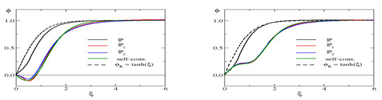
Figure 1.
Profiles for and . (Left panel): configuration, (Right panel): . The full black line (labeled ) arises from minimizing the total energy, Equation (16). The other lines (, , self-cons.) are configurations obtained from minimizing the reduced energy functional, Equation (19). The legends refer to the notation of Table 1 and Table 2. For completeness, we also show the kink without any fermion interaction (dashed lines).
We will now elaborate on our numerical analysis of scanning the g- space in more detail. With the VPE included, even the configuration has a non-zero fermion energy6 and thus a deviation is expected. We will discuss this case first although a very similar setting has already been considered in Ref. [19].
For the configuration, the kink, has , where and for and , respectively. For the cases shown in Table 3, the variational minimum is only slightly less than the total energy of the kink. Again, this corroborates the assertion that the inclusion of the fermion fields only leads to a moderate back-reaction. We also see that for the case which is thus kinematically stable against a decay into a free fermion. However, since the zero mode does not have definite fermion charge, this configuration cannot be asserted as a particle number, in contrast to a free fermion.
Table 3.
Variational approach for the configuration. Top panel: , bottom panel: . The valence contribution is not listed as for this configuration. For comparison, we also list the total energy for the kink profile .
Next, we turn to the configuration with the numerical results displayed in Table 4.
Table 4.
Variational approach for the configuration. Top panel: , bottom panel: . The entries and are those of Table 2.
In this case, the valence energy is substantial. However, since a strongly distorted kink comes with large and , cf. Table 1, minimizing the valence energy does not lower the total energy. Rather, configurations that minimize the total energy have significantly larger valence energies than the solutions constructed in Refs. [10,11,12]. The resulting configuration is similar to the kink as the variational parameters approximately obey and . We find that c is slightly larger than unity which would indicate that profile is a squeezed kink. However, the remaining differences between a and d as well as between b and e lead to a stretched kink. This is seen in Figure 1 in which we show minimizing profiles for various channels. As we increase , the classical contribution to the energy becomes more dominant and the minimizing configuration should come even closer to the kink. Indeed, the numerical simulations confirm this as we find the variational parameters and for and , respectively, with in both cases. The respective energies are and . The discrepancies with the energy of the kink configuration ( and ) are marginal and decrease as increases.
As a final example, we consider the configuration when the valence fermion dwells in the third bound state, the second one with even parity. The numerical results are displayed in Table 5.
Table 5.
Variational approach for the configuration. Top panel: , bottom panel: . The entries and are those of Table 2.
The scenario is basically the same as for the previous configurations: The inclusion of the fermion VPE moves the distorted kink back to a slightly stretched kink. We see that even for the variational solution is not very different from the kink. This implies that the total energy is dominated by the classical part which is another indication that there are sizable cancellations between the gain from binding a valence fermion and the fermion VPE. All our variational searches yield so that the profile approaches the vacuum expectation value from above as .
For a certain parameter set, we display the profiles that minimize in the various channels in Figure 2.
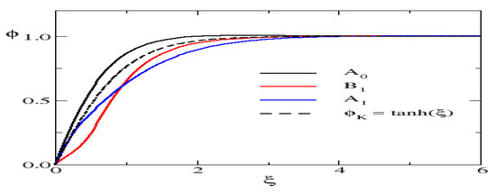
Figure 2.
Variational solutions of the , and configurations for and . For comparison, the kink profile is also shown.
When compared to the kink, the solution of the configuration is squeezed, while the others are stretched. The reason for this is that squeezing the kink slightly decreases the VPE. To considerably gain energy from binding a non-zero mode, the Yukawa interaction must be strongly attractive which requires an extended kink profile. That is what we observe for the and configurations.
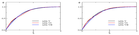
We should, however, mention that we find various local minima for the total energy in the space of the chosen variational parameters. Their total energies may be slightly smaller or larger than those reported above but they turn out to be stationary under the steepest descent algorithm. This is the case for all configurations but we will discuss this only for the configuration in more detail. The data for some of the alternative solutions are listed in Table 6 and Table 7. Looking at the corresponding variational parameters suggests that these solutions would be quite different. In particular, those from Table 6 exhibit significant deviations from the kink relation . However, when plotting them, cf. Figure 3, we observe that the profiles are approximately identical and differences become smaller as the Yukawa coupling increases. We conjecture that these solutions are fairly close to the actual solution but the particular variational ansatz is not capable of capturing it exactly. Furthermore, the minimum may be very shallow. The ansatz most likely does not allow for a continuous transition between the solutions on a path that can be constructed from a steepest descent procedure. In any event, we have sufficient evidence to state that the actual solution will be similar to the kink but quite distinct from the solutions of Refs. [10,11,12]. The latter could emerge for model parameters for which the classical and/or Dirac sea contributions, which both prefer the standard kink profile, are suppressed compared to the valence part. Equation (16) reveals that such parameters are governed by small for which the present semi-classical expansion is not reliable.
Table 6.
Alternative solutions for the configuration: Top panel , bottom panel .
Table 7.
Second set of alternative solutions for the configuration: Top panel , bottom panel .
Without the fermion coupling, the boson contribution to the VPE is for [25,31,32]. With that coupling included, the boson VPE is difficult to estimate because there is a linear term in the harmonic approximation for the fluctuations when the profile is not a solution to the classical kink equation. Furthermore, imaginary frequency eigenvalues emerge for the boson fluctuations [33]. Yet, we assume that the above number is a useful estimate because the variational profiles are quite similar to the kink. As conjectured earlier, the numerical simulations verify that the fermion VPE becomes significantly larger when the Yukawa coupling increases. In Section 3.1, we especially argued that for large-enough values of the Yukawa coupling constant, the fermion VPE should dominate the boson counterpart. And indeed, we always find that when .
5. Conclusions
In this project we have considered a model with fermions coupled to the kink in one space and one time dimension and investigated the fermion back-reaction on the kink profile. In this approach a valence fermion appears as an explicitly occupied bound state level and the back-reaction may be significant when this is not the ground state level. And indeed, earlier studies which only considered the coupling of the kink to a single fermion valence level found considerable back-reactions. However, it is important to not only consider the energy of the occupied valence level but also to add the energy of the Dirac sea to the functional that determines the back-reaction. The main argument for its inclusion is the consistency of the semi-classical expansion. This contribution is obtained as the renormalized sum of the changes of the one-particle fermion energies. These changes emerge because the Yukawa coupling between the kink and the fermions polarizes the fermion vacuum. They concern the discrete bound states as well as the continuous scattering states. The boson contribution to the vacuum polarization energy has not been included in the energy functional. Rather, we have argued that for large values of the Yukawa coupling constant, the fermion energies would dominate the quantum corrections. We have verified that conjecture a posteriori.
We have utilized a variational approach to find an upper bound to the minimal total energy. We have only considered a single variational parameterization of the kink profile with five parameters to lessen the numerical efforts. Certainly, this leaves space for improvement. Nevertheless, we consider it sufficient to show that the Dirac sea contribution brings back the strongly distorted kink profiles from the self-consistent treatment for the case that omits the Dirac sea, to a slightly squeezed or stretched kink profile. The similarity to the kink is particularly pronounced for the configuration where we do not have a valence quark contribution to the energy. For that reason, a slightly squeezed kink profile is energetically favorable for the configuration. In all other cases, some energy is gained from binding the valence level by stretching the kink because it makes the Yukawa interaction more attractive. Since this deformation increases both the classical energy and the vacuum polarization energy, the stretch can only be modest.
The dominant effect for mitigating the kink distortion is the balance between the fermion bound state and vacuum energies so that the profile function is governed by minimizing the classical energy. This balance could well be a consequence of Levinson’s theorem [34,35], which relates the number of bound states to the density of continuum states. Essentially, it states that any bound state must have emerged from the continuum so that there is an exact balance between bound and scattering states when the background potential changes. The fermion energy has two contributions, the valence part which arises from the bound state energies and the vacuum polarization energy, which results from the scattering data. For the energies, the balance is not exact because the particle number (density) carries factors of the single-particle energies. Nevertheless, the theorem strongly suggests that the energy gain from one comes with an energy loss of the other.
Though kink-type solutions emerge in many field theories, systems with explicit scalar and fermion fields are most prominent in variants of the standard model of particle physics. When embedded in three space dimensions, kinks represent domain walls in those models [6]. In these models, the fermions’ back-reaction on the kink may eventually exhibit effects like those we have explored here, in particular when the fermions are bound by the domain wall and dwell in excited levels.
We have considered cases in which only a single fermion occupation number was non-zero. The valence energy should become more important when this is true for several occupation numbers. Then, we expect a stronger distortion of the kink. This should be the subject of future projects.
Author Contributions
The authors mutually agree that their contributions warrant co-authorship. All authors have read and agreed to the published version of the manuscript.
Funding
H.W. is supported in part by the National Research Foundation of South Africa (NRF) by grant 150672.
Data Availability Statement
All relevant data is contained within the article.
Conflicts of Interest
The authors declare no conflicts of interest.
Notes
| 1 | In physical variables the separation leading to the stationary equation is . |
| 2 | The computations of Ref. [27] make ample use of scattering data; so do we. Additionally we use the analytic properties of the Jost function to write the VPE as a single integral over imaginary momenta. Note also that Ref. [27] computes the VPE for two widely separated kinks and therefore has an additional factor two in Equation (21). |
| 3 | There have been attempts to pursue that program [29], however, the relation between the gauge invariant proper-time regularization and the sharp cut-off for is unclear. |
| 4 | We write absolute values for the odd powers to maintain the reflection property . The actual calculation is performed on the half-line and the absolute value sign can be ignored. |
| 5 | This is similar to the S-wave bound states for the Coulomb problem in the Schrödinger equation. |
| 6 | The bound state by itself is a zero mode with either u or v vanishing so that and thus does not couple to the scalar field. |
References
- Nambu, Y. String-Like Configurations in the Weinberg-Salam Theory. Nucl. Phys. B 1977, 130, 505. [Google Scholar] [CrossRef]
- Weigel, H. Chiral Soliton Models for Baryons; Lecture Notes in Physics; Springer: Berlin/Heidelberg, Germany, 2008; Volume 743. [Google Scholar]
- Feist, D.T.J.; Lau, P.H.C.; Manton, N.S. Skyrmions up to Baryon Number 108. Phys. Rev. D 2013, 87, 085034. [Google Scholar] [CrossRef]
- Schollwöck, U.; Richter, J.; Farnell, D.J.J.; Bishop, R.F. Quantum Magnetism; Lecture Notes in Physics; Springer: Berlin/Heidelberg, Germany, 2004; Volume 645. [Google Scholar]
- Nagaosa, N.; Tokura, Y. Topological properties and dynamics of magnetic skyrmions. Nat. Nanotech. 2013, 8, 899. [Google Scholar] [CrossRef] [PubMed]
- Vilenkin, A.; Shellard, E.P.S. Cosmic Strings and Other Topological Defects; Cambridge University Press: Cambridge, UK, 2000. [Google Scholar]
- Moradi Marjaneh, A.; Simas, F.C.; Bazeia, D. Collisions of kinks in deformed l. 160 φ4 and l. 160 φ6 models. Chaos Solitons Fractals 2022, 164, 112723. [Google Scholar] [CrossRef]
- Chu, Y.Z.; Vachaspati, T. Fermions on one or fewer kinks. Phys. Rev. D 2008, 77, 025006. [Google Scholar] [CrossRef]
- Brihaye, Y.; Delsate, T. Remarks on bell-shaped lumps: Stability and fermionic modes. Phys. Rev. D 2008, 78, 025014. [Google Scholar] [CrossRef]
- Klimashonok, V.; Perapechka, I.; Shnir, Y. Fermions on kinks revisited. Phys. Rev. D 2019, 100, 105003. [Google Scholar] [CrossRef]
- Perapechka, I.; Shnir, Y. Kinks bounded by fermions. Phys. Rev. D 2020, 101, 021701. [Google Scholar] [CrossRef]
- Saadatmand, D.; Weigel, H. Excited fermions on kinks and the Dirac sea. Phys. Rev. D 2023, 107, 036006. [Google Scholar] [CrossRef]
- Alkofer, R.; Reinhardt, H.; Weigel, H. Baryons as chiral solitons in the Nambu-Jona-Lasinio model. Phys. Rept. 1996, 265, 139. [Google Scholar] [CrossRef]
- Friedberg, R.; Lee, T.D. Fermion Field Nontopological Solitons. 1. Phys. Rev. D 1977, 15, 1694. [Google Scholar] [CrossRef]
- Kahana, S.; Ripka, G.; Soni, V. Soliton with Valence Quarks in the Chiral Invariant Sigma Model. Nucl. Phys. A 1984, 415, 351. [Google Scholar] [CrossRef]
- Jain, P.; Johnson, R.; Schechter, J. Aspects of the Chiral Quark Model. Phys. Rev. D 1988, 38, 1571. [Google Scholar] [CrossRef] [PubMed]
- Callan, C.G., Jr. Dyon-Fermion Dynamics. Phys. Rev. D 1982, 26, 2058. [Google Scholar] [CrossRef]
- Nolte, G.; Kunz, J. The Sphaleron barrier in the presence of Fermions. Phys. Rev. D 1993, 48, 5905–5916. [Google Scholar] [CrossRef] [PubMed][Green Version]
- Farhi, E.; Graham, N.; Jaffe, R.L.; Weigel, H. Heavy fermion stabilization of solitons in (1+1)-dimensions. Nucl. Phys. B 2000, 585, 443. [Google Scholar] [CrossRef]
- Farhi, E.; Graham, N.; Jaffe, R.L.; Weigel, H. Searching for quantum solitons in a (3+1)-dimensional chiral Yukawa model. Nucl. Phys. B 2002, 630, 241–268. [Google Scholar] [CrossRef][Green Version]
- Chodos, A.; Jaffe, R.L.; Johnson, K.; Thorn, C.B.; Weisskopf, V.F. A New Extended Model of Hadrons. Phys. Rev. D 1974, 9, 3471. [Google Scholar] [CrossRef]
- Bowler, K.C.; Hey, A.J.G. The Roper Resonance: A Problem for the MIT Bag? Phys. Lett. B 1977, 69, 469. [Google Scholar] [CrossRef]
- Guichon, P.A.M. A Nonstatic Bag Model for the Roper Resonances. Phys. Lett. B 1985, 164, 361. [Google Scholar] [CrossRef]
- Reinhardt, H. The Chiral Soliton in the Proper Time Regularization Scheme. Nucl. Phys. A 1989, 503, 825. [Google Scholar] [CrossRef]
- Graham, N.; Quandt, M.; Weigel, H. Spectral Methods in Quantum Field Theory; Lecture Notes in Physics; Springer: Berlin/Heidelberg, Germany, 2009; Volume 777. [Google Scholar]
- Faulkner, J.S. Scattering theory and cluster calculations. J. Phys. 1977, C10, 4661. [Google Scholar] [CrossRef]
- Graham, N.; Jaffe, R.L. Fermionic one loop corrections to soliton energies in (1+1)-dimensions. Nucl. Phys. B 1999, 549, 516. [Google Scholar] [CrossRef]
- Graham, N.; Weigel, H. Quantum corrections to soliton energies. Int. J. Mod. Phys. A 2022, 37, 2241004. [Google Scholar] [CrossRef]
- Diakonov, D.; Polyakov, M.V.; Sieber, P.; Schaldach, J.; Goeke, K. Sphaleron transitions in the minimal standard model and the upper bound for the Higgs mass. Phys. Rev. D 1996, 53, 3366. [Google Scholar] [CrossRef] [PubMed]
- Baker, G.A., Jr. Padé approximant. Scholarpedia 2012, 7, 9756. [Google Scholar] [CrossRef]
- Dashen, R.F.; Hasslacher, B.; Neveu, A. Nonperturbative Methods and Extended Hadron Models in Field Theory 2. Two-Dimensional Models and Extended Hadrons. Phys. Rev. D 1974, 10, 4130–4138. [Google Scholar] [CrossRef]
- Rajaraman, R. Solitons and Instantons; North Holland: Amsterdam, The Netherlands, 1982. [Google Scholar]
- Graham, N.; Jaffe, R.L. Unambiguous one loop quantum energies of (1+1)-dimensional bosonic field configurations. Phys. Lett. B 1998, 435, 145–151. [Google Scholar] [CrossRef]
- Levison, N. On the uniqueness of the potential in a Schrödinger equation for a given asymptotic phase. Kgl. Dan. Vidensk. Selsk.-Mat.-Fys. Medd. 1949, 25, 9. [Google Scholar]
- Barton, G. Levinson’s Theorem in One-dimension: Heuristics. J. Phys. A 1985, 18, 479–494. [Google Scholar] [CrossRef]


Disclaimer/Publisher’s Note: The statements, opinions and data contained in all publications are solely those of the individual author(s) and contributor(s) and not of MDPI and/or the editor(s). MDPI and/or the editor(s) disclaim responsibility for any injury to people or property resulting from any ideas, methods, instructions or products referred to in the content. |
© 2023 by the authors. Licensee MDPI, Basel, Switzerland. This article is an open access article distributed under the terms and conditions of the Creative Commons Attribution (CC BY) license (https://creativecommons.org/licenses/by/4.0/).