Abstract
We study the interaction of two discrete pomeron fields while considering mass mixing and the general structure of the interaction potential for pomerons within the framework for a functional renormalization group analysis of Reggeon field theory. We find fixed points from the zeros of the beta function establishing the existence of three groups of solutions: the first corresponds to two uncoupled pomerons, the second is a solution known as a “pomeron–odderon” interaction, and the final is a real general solution with an interaction potential. We also study its universal properties around this fixed point. This analysis allows for a discussion for the first time on the mixing of two pomerons through renormalization flow paths from the ultraviolet to the non-perturbative infrared regions. Finally, we comment on its role in high-energy scattering.
1. Introduction
The Regge limit of high-energy QCD remains a topic of high interest. At small transverse distances, where perturbation theory can be applied, QCD predicts the BFKL pomeron [1,2,3,4,5], which is characterized by an intercept and slope . In this kinematic region (where the energy is bigger than the transferred momenta), the scattering process is described through the exchange of pomerons.
In QCD at NLO, when the strong coupling becomes momentum-dependent, an infrared cutoff has to be introduced, which, strictly speaking, already goes beyond perturbation theory, and the BFKL pomeron spectrum becomes discrete, even at relatively short distances. Then, we need to investigate which of them and in what way they will contribute to the scattering processes at large distances and rapidity.
To study the interactions of these Regge poles, it is convenient to consider a local approximation for the action and make use of the well-established formalism of Reggeon field theory (RFT) [6,7,8], which lives in -dimensions, transverse momenta. This approach significantly simplifies the inclusion of pomeron interactions, and as a comprehensive QCD description, pomerons are Reggeized gluons and their interactions are characterized by non-local vertex functions [9,10,11]. Then, RFT offers a robust description of strong interactions in the Regge limit and infrared region. In Regge theory, a pomeron appears like singularities (i.e., cuts and poles) in the angular momentum -complex plane. Thus, we should not find Reggeons between and the -cut.
With an infrared cutoff and running , the -cut segment between the -cut and zero is replaced by an infinite sequence of discrete poles accumulating at zero. This scenario has been confirmed in numerical studies for various infrared cutoff versions: in [12], an infrared cutoff is introduced, preserving the BFKL bootstrap property (related to s-channel unitarity); in [13,14,15], boundary values of the BFKL amplitude are imposed at a fixed momentum scale ; in [16,17,18], a Higgs mass is used as an IR regulator; and in [19], a more sophisticated regulator is introduced, embedding the BFKL pomeron into Wilsonian exact renormalization group techniques.
Furthermore, for this discrete spectrum part, the eigenfunctions have been studied [20,21]: notably, only for the leading eigenvalue is the wave function centered in the “soft” region of small transverse momenta, while for the nonleading eigenvalues, the wave functions become “hard”, i.e., these pomeron states are centered in the UV region of large transverse momenta. The remaining task is the “unitarization” of this set of pomeron states, requiring, in particular, the introduction of the triple pomeron vertex [22].
To study the transition from the ultraviolet (UV) to the infrared (IR) regions, to move to larger distances, we choose the IR-regulated effective action, satisfying functional renormalization group (FRG) equations, as the method to encode the different dynamical regimes.
The finite set of discrete BFKL pomerons (accumulating at ) was used [23] to fit the small-x and low- HERA data, allowing for a good description. In this previous analysis, no attempt was made to introduce the triple pomeron vertex. In this paper, our goal is to embed the discrete BFKL pomerons into Reggeon field theory, incorporating corrections to the BFKL pomeron interaction vertices in the potential, in particular, the pomeron triple vertex.
The next step is the introduction of an infrared regulator, which later on will allow us to make use of the exact renormalization group approach. We describe how to implement this regulator for the effective interaction of the N-discrete BFKL pomeron and derive the renormalization equation for the parameters defined in the BFKL pomeron effective action concerning the IR cutoff parameter k. We obtain nonlinear evolution equations for the intercepts, slopes, and coupling constants.
In this research, we study the interaction of two pomerons as first approximations, starting with an effective potential with a non-diagonal intercept between the pomerons. This first approximation is crucial for understanding the necessary steps to derive the flow equation using the Wetterich flow equation for a general effective action for N-pomeron interactions. As we know, FRG at a low approximation can be restricted to one-loop calculations, enabling us to determine the critical properties of the theory at one loop. However, in a recent paper, Braun [24] studied the renormalization group (RG) approach for the pomeron–odderon model in two transverse dimensions in the single one-loop approximation and found similar results to those we obtained using the functional renormalization approach [25]. One of the important results show that the single-loop approximation adopted is not sufficient but provides a relatively good understanding of the theory’s behaviour.
In our papers [19,25], we initiated an analysis of the flow equations of Reggeon field theory (RFT) and employed the Wetterich formulation of the functional renormalization group equations [26,27] to directly study the problem in two transverse dimensions. As the main result of our research is the establishment of a critical theory (fixed point) in this multidimensional parameter space of the effective potential, there are directions that are IR-attractive (UV-repulsive), while all other directions are UV-attractive. We have verified that such a fixed point is related to the same universal class as the percolation model in statistical physics [28]. This equivalence with models of non-equilibrium physics potentially impacts the statistical physics of generalized multicomponent-directed percolation models and start to increase the interested in this theory [29,30].
Self-interactions of the pomeron [31] and interactions between the pomeron and odderon are naturally present in perturbative QCD analyses [22]. Similar findings have also been obtained in the Colour Glass Condensate and dipole approaches [32,33,34].
This paper is organized as follows: We first describe the general setup and then present our fixed point analysis results as the zeros of the functions. In the final part, we calculate the trajectory of the physical parameter for the pomerons around the fixed point, allowing us to define the pomeron intercepts and offer the first hint at a physical interpretation.
2. The General Setup
To investigate the critical properties of a discrete pomeron interaction, we use the functional renormalization group approach, which has been successfully applied to different areas: in statistical mechanics, particle physics, and quantum gravity (for a review, see [35,36,37]).
In brief, in this FRG approach, the study of the effective action needs the introduction of an infrared regulator , which controls the range of modes integrated out. One of the main goals of this research is to find fixed points of the flow equation which must be solved using analytic or numerical approximations.
2.1. The Action and the Flow Equation
In 1967, Gribov [38] developed rules for calculating Feynman diagrams in processes involving Reggeons. Inspired by this work, effective field theories were developed to derive these rules through an effective action [39].
In the context of QCD, a pomeron is generated as a composite state of two or more Reggeized gluons; however, in RFT, Reggeons are represented by fields , as proposed in [7,25]. The effective action for N different Reggeons is given by the following expression:
where is the time (rapidity); is the dimension of transverse space (both variables are conjugate to Reggeon energy and transverse momenta k); is the renormalization wave function; is the slope of the corresponding Reggeon’s; and are the “mass” parameters of the fields, related to the intercepts of the Regge trajectories as ; are the couplings associated with the potential; and , where n is the number of couplings in the potential.
In previous works, we have studied actions of the form (1) with , calculating the functions using the Wetterich equation. These studies include a self-interacting field pomeron [19] and two fields interacting: pomeron–odderon with cubic terms in the potential [25] that consider the signature and parity constraints of the fields. Both were expanded using the local potential approximation (“LPA”) for small fields.
The interaction between the two pomerons discrete fields is described by the cubic potential :
and the effective action is as follows:
To find the critical properties of the pomeron interaction, we need to determine the flow equation of the effective action using the FRG.
2.2. Functional Renormalization Group Equation
The functional renormalization group equation, or the Wetterich equation, is given by the following:
where the renormalization time evolution t is , , and . In order to compute the rhs of the flow equations, which results from scale -controlled contributions from quantum fluctuations, we find it convenient to expand in the following way:
Here, is the inverse of . This matrix is not diagonal, and introducing the variable , the propagator for is given by the following:
Then, we need to consider that the trace in the Equation (4) extends over a matrix, and needing a regulator, we chose the optimized Litim regulator [40] as follows:
allowing for a simple analytic integration in the closed form.
The matrix propagator is written as
with block matrices defined as
and so on for , , and . Finally, the interaction potential matrix in Equation (6) is defined as:
where the derivatives of the potential with respect to the fields excluded intercept terms.
With all elements defined, we proceed to solve the Wetterich equation for the action shown in Equation (3). Only contains a q dependence for . Therefore, the momentum integrals considering the Litim regulator are direct. The energy -integral is computed using complex integration. Employing a weak field polynomial expansion and dimensionless variables, the functions are obtained by taking derivatives with respect to field variables in the Wetterich equation and subsequently setting the fields to zero.
2.3. Functions
We start by introducing dimensionless variables. The field variables and parameters are rescaled as follows:
which are then substituted into action (3). The functions will be differential equations with respect to . It is useful to introduce the new parameter , and it will provide us with an additional equation:
where are some of the anomalous dimensions. Introducing this parameter and its respective differential equation will allow us to have the same number of differential equations as variables. We will also define the anomalous dimensions , along with
The consist of two parts: one canonical part related to a classical term derived from the dimensional analysis of equations dependent on anomalous dimensions and couplings and the other from Equation (4) related to radiative corrections dependent on coupling constants and “mass” terms. After simplifying our results, the general forms of the functions are as follows:
where represents certain functions with poles at and . The expressions for f’s (i.e., radiative corrections) in the functions have a diagrammatic representation. These expressions are already lengthy and will not be listed here (they are available at https://www.wolframcloud.com/obj/luis.cancinoa/Published/FuFunciones_Beta.nb, accessed on 14 February 2024).
The Equations (14)–(19) cannot be solved without the determination of the anomalous dimensions . To obtain the anomalous dimensions, we proceed in the following way: first, we determinate the two-point vertex functions.
Then, we take derivatives with respect to energy
and momentum
The anomalous dimensions are then given by the following:
To verify this expressions, we take the limit to the pomeron–odderon case and we obtain expressions that coincide with those found in [25] (more details can be found in this ref.). Finally, the functions are obtained by direct calculation. Let us comment that the evolution equation for r becomes indicating that at criticality, the pomeron’s transverse space scaling laws coincide.
3. Numerical Results
In this section, we address the numerical challenges associated with solving the functions and identifying fixed points (FPs), which are the zeros of the functions. To numerically find FPs, one common method is the Newton–Raphson method or its modified variants. These methods are required to be close to the FP for high precision. However, working in a 10-dimensional space can be complex and computationally intensive. We identified an alternative method with improved convergence properties. The algorithm developed by Li and Zeng [41] demonstrates good convergence for finding FPs using random points in the theory space. After identifying the FPs, we linearized the system around them and calculated the critical exponents using the stability matrix. We then focused on points of interest, primarily those acting as attractors in the infrared (IR) regime.
3.1. Fixed Points
Therefore, we will present the results of the FPs for the functions in the case where all anomalous dimensions are nonzero, verifying that the points are solutions to these functions. We found many different fixed points, which can be real or complex and are not fully IR-attractive. We will concentrate only on the real ones and study their behaviour in the vicinity of the fixed points.
Now, we turn to the calculation of the fixed points; the zeroes of the -functions; the anomalous dimensions , ; and the degree of stability of each fixed point, which is determined by the sign of the eigenvalues of the stability matrix (first derivatives of the -function: ), computed at the fixed point. In the phase space, there are directions of instability for each negative real part of the eigenvalues in the infrared limit and stabilities for the case of positive real part eigenvalues. We have found several different solutions (omitting all solutions with negative r).
(a) For the first solution, we have , , and , and only the two couplings and are different from zero: this corresponds to two decoupled pomerons [19]:
Furthermore, the anomalous dimensions are as follows:
(b) We find that a second solution—which has the same structure as the “pomeron–odderon” discussed in [25]—has , , and , and only the coupling , is nonzero:
Furthermore,
(c) We also found other solutions where we have , , and m, and all the couplings are different from zero, which is given by the following:
For the anomalous dimensions, we found
The spectral analysis of the stability matrix at this fixed point is able to show the other universal quantities of the system. This solution has a higher infrared stability, and the eigenvalues from the stability matrix are
In particular, we found four negative eigenvalues and six positive eigenvalues associated with six relevant directions. From the stability matrix, there exist six eigenvectors that span the subspace of the six pomeron parameters, which have positive eigenvalues, i.e., this subspace is part of the 10-dimensional critical subspace. Inside this subspace, they are orthogonal to all other four eigenvectors with negative eigenvalues.
We then analysed, for this special fixed point, the behaviour of the pomerons parameters and studied some trajectories of the flow equation.
We also found more solutions where all couplings are nonzero, and the eigenvalues of the stability matrix are complex-valued, and their real parts are negative; then, the fixed points are IR unstable, and we will not consider those solutions.
3.2. Evolution of Two Pomerons and Dynamics around Fixed Points
Our fixed point analysis was conducted in the space of dimensionless parameters, revealing distinct behaviours for the flow of physical (dimensionful) parameters. For the two-pomeron system, we performed numerical studies of the flow for dimensionless parameters. Starting in the UV region within the critical subspace, we end up at the fixed point in the IR limit, where both pomerons have equal slopes.
The study of flows in the theory space allows us to observe how the system evolves with respect to t. Identifying two states of the pomeron family and examining the connecting flow is crucial for our objectives. However, the challenge lies in working within a 10-dimensional space. At most, we can visualize projections in three dimensions, with numerous possible combinations. Hence, controlling deviations around the fixed point (FP) is essential. We selected the ones with the most attractive eigenvalues in the infrared since we are interested in points that may represent a limit in the non-perturbative region.
In exploring the evolution of different pomeron states, we focus on the intercept subspace’s parameters (, , and m). Each flow associated with these points shows distinct behaviours for the intercepts (, ) and m. After selecting the region for analysis, we examine the parameter behaviour as each coupling varies, generating different trajectories, which correspond to a different initial conditions of . To generate the different trajectories, we discretize the functions as . The initial conditions are fixed at , allowing us to study the behaviour in the UV for positive t values and in the IR for negative t values. This procedure helps us identify a group of trajectories from the renormalization group equation.
We have found several stable trajectories, from which we are selecting only six of them (represented by different colours in Figure 1 and Figure 2), which are generated by adding a small parameter in each initial condition. The six trajectories allow us to describe the behaviour of the , , , and near the fixed point, as shown in Figure 1. Figure 2 displays the evolution of the intercepts for this group of trajectories near the fixed point. The trajectories approach the fixed point and then diverge as t increases, with the UV directions starting to dominate.
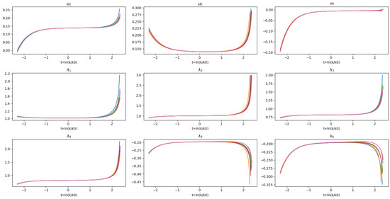
Figure 1.
Graphs represent time evolution of the dimensionless pomeron parameters: , , , and , which are shown at the top of each one of them, in the neighbourhood of the fixed point (Notice that the time evolution t is dimensionless). The colours of the lines in the graphs represent different trajectories generated by the procedure of small variations in the initial condition of .
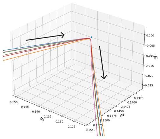
Figure 2.
The graphic shows the time evolution of the dimensionless mass parameter (i.e., , , and m, which are dimensionless), which is also observed in a projection in the “mass” spaces considering the behaviour shown in Figure 1. The arrows indicate where the system evolves in the IR limit (i.e., negative t).
3.3. Mass Matrix Diagonalization
The primary motivation for studying the flow of the renormalization group equation in this work, particularly in the context of distinct states for the pomeron, is to find a path that connects two of these states while changing the scale. Recall the discussion in the theoretical framework, where it is explained that the soft-pomeron [42] dominates in the infrared (IR), while the hard-pomeron [19] dominates in the ultraviolet (UV). Due to the complexity of finding these paths in the 10-dimensional space, we focus on the “mass” parameters. Then, we analyse how the “mass” matrix diagonalizes when trajectories are close the FP. We examine the evolution (from the UV) of a state with to the fixed point as it progresses towards the IR (states with ). We concentrate on the action restricted to the pomerons’ intercepts, which the flow equation indicates are not diagonal.
In the vicinity of the FP, we have a non-diagonal matrix. The final pomeron intercepts are the eigenvalues of this matrix. The evolution of the dimensionfull eigenvalues of the intercept matrix are shown in Figure 3, and the value at the fixed point are . As an initial condition at , we use the points defined in the previous subsection, showing how they evolve towards the IR (t-negative) and the UV (t-positive).
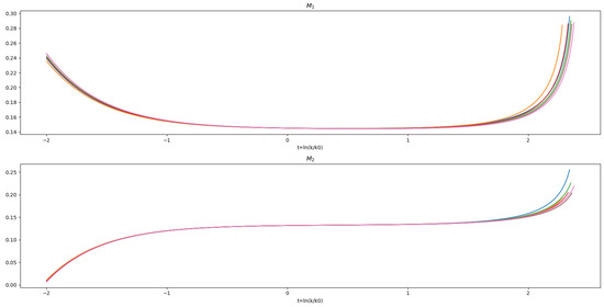
Figure 3.
The graphs show the evolution of the diagonalized dimensionless “masses” (i.e., and ), and their behaviour is quite similar to that of the intercepts and shown earlier.
The eigenvectors allow us to see the contribution of each original field in terms of the “masses”, and how each contribution evolves in the theory space.
With this method of generating the eigenvectors, we observe that, in the limit (and ), the new fields are equal to the original ones, i.e., and . The points selected in the previous subsection were chosen to observe this behaviour in more detail.
Finally, to establish a connection between two pomeron states, we diagonalized the “mass” matrix and identified a configuration where the fields were decoupled () in the UV. We obtained different trajectories that evolved towards the fixed point in the IR, as shown in Figure 4. These figures illustrate the evolution of the mixing of the pomerons, starting in the UV with one pomeron state, and they mixed as the trajectories evolved towards the IR.
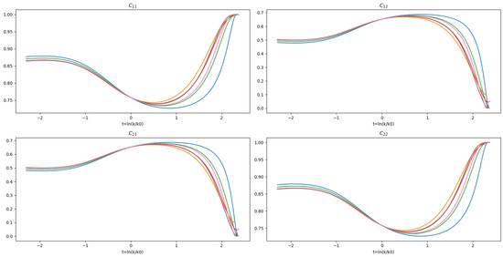
Figure 4.
The graphs show how different flow lines converge to a state where the dimensionless “masses” mixed. If we start with the initial condition, the masses do not mix (i.e., ), and through the flow equations evolving towards the IR, the fields start mixing, passing through the fixed point and converging into another state in the IR (notice that t is dimensionless too).
4. Conclusions
In this study, we have extended our previous analysis of fixed points in pomeron Reggeon field theory by incorporating a system of interacting discrete pomeron fields, especially in the infrared limit. Our results describe significant aspects of these interactions of two pomerons, which contribute to a deeper understanding of the complex dynamics in pomeron field theories.
The main result of our investigation is the identification of three different solution: one corresponds to two uncoupled pomerons, the second solution corresponds to a pomeron/odderon interaction, and the new real solution corresponds to a full interaction potential. From the spectral analysis of the stability matrix, we found the critical properties of the theory and we have six relevant directions. These directions exhibit IR stability, while the remaining eigenvalues indicate UV-stable directions. Particularly, we observed that, in the effective potential’s parameter space, the relevant directions define a critical subspace. Starting within this subspace at a nonzero scale k, the system invariably approaches the infrared stable fixed point as k tends to zero. Conversely, initiating the system outside the critical subspace but in proximity to the fixed point results in an attraction towards the relevant direction, moving the system away from the fixed point.
Furthermore, from our analysis, we have been able to analyse for the first time the mixing of two pomerons through the renormalization flow trajectory from the UV to the nonperturbative IR regions. The IR fixed point structure confirms the persistence of the two pomerons through the flow from UV to IR. This observation is crucial for understanding the survivability and robustness of these states under scale transitions. Additionally, our analysis offers insights into the interactions between two discrete pomeron fields, including the suppression of one pomeron in favour of another exchange. Such information is critical for comprehending the competitive dynamics among different Reggeon fields.
Finally, our results can be applied to other physics topics too. For example: Given the equivalence among RFT and directed percolation models, our analysis could be used to study the critical property in multifield extensions of those statistical models. In addition, considering our results about the superposition of the finite set of discrete BFKL pomerons, another natural application could be to fit small-x and low- experimental HERA data.
Author Contributions
All authors contributed equally to this work. All authors have read and agreed to the published version of the manuscript.
Funding
This research was supported by Fondecyt (Chile) grant 1231829, and L.C. is thankful for the grant PIIC (“Programa de Incentivo a la Iniciacion Cientifica”) from UTFSM.
Data Availability Statement
The data presented in this study are available from the corresponding author on request.
Acknowledgments
We thank to J. Bartels for the encouraging discussions.
Conflicts of Interest
The authors declare no conflicts of interest.
References
- Lipatov, L.N. Reggeization of the vector meson and the vacuum singularity in non-Abelian gauge theories. Sov. J. Nucl. Phys. 1976, 23, 338–345. [Google Scholar]
- Kuraev, E.; Lipatov, L.N.; Fadin, V. Multi-reggeon processes in the Yang-Mills theory. Phys. Lett. B 1975, 60, 50–52. [Google Scholar]
- Kuraev, E.; Lipatov, L.N.; Fadin, V. Multi-reggeon processes in the Yang-Mills theory. Sov. Phys. JETP 1976, 44, 443–450. [Google Scholar]
- Kuraev, E.; Lipatov, L.N.; Fadin, V. The Pomeranchuk singularity in non-Abelian gauge theories. Sov. Phys. JETP 1977, 45, 199–204. [Google Scholar]
- Balitsky, I.; Lipatov, L.N. The Pomeranchuk singularity in quantum chromodynamics. Sov. J. Nucl. Phys. 1978, 28, 822–829. [Google Scholar]
- Gribov, V.N.; Migdal, A.A. Strong Coupling in the Pomeranchuk Pole Problem. Sov. Phys. JETP 1969, 28, 784–795. [Google Scholar]
- Abarbanel, H.D.; Bronzan, J.B. Structure of the Pomeranchuk Singularity in Reggeon Field Theory. Phys. Rev. D 1974, 90, 2397. [Google Scholar] [CrossRef]
- Moshe, M. Recent Developments in Reggeon Field Theory. Phys. Rep. 1978, 37, 255–345. [Google Scholar] [CrossRef]
- Braun, M.; Vacca, G.P. Triple pomeron vertex in the limit N(c) —> infinity. Eur. Phys. J. C 1999, 6, 147–157. [Google Scholar] [CrossRef]
- Bartels, J.; Ryskin, M.G.; Vacca, G.P. On the triple pomeron vertex in perturbative QCD. Eur. Phys. J. C 2003, 27, 101–113. [Google Scholar] [CrossRef]
- Bartels, J.; Braun, M.; Vacca, G.P. Pomeron vertices in perturbative QCD in diffractive scattering. Eur. Phys. J. C 2005, 40, 419–433. [Google Scholar] [CrossRef]
- Braun, M.; Vacca, G.P.; Venturi, G. Properties of the hard pomeron with a running coupling constant and the high-energy scattering. Phys. Lett. B 1996, 388, 823–831. [Google Scholar] [CrossRef][Green Version]
- Kowalski, H.; Lipatov, L.N.; Ross, D.A.; Schulz, O. Decoupling of the leading contribution in the discrete BFKL Analysis of High-Precision HERA Data. Eur. Phys. J. C 2017, 77, 777. [Google Scholar] [CrossRef]
- Kowalski, H.; Lipatov, L.N.; Ross, D.A. The Behaviour of the Green Function for the BFKL Pomeron with Running Coupling. Eur. Phys. J. C 2016, 76, 23. [Google Scholar] [CrossRef]
- Kowalski, H.; Lipatov, L.N.; Ross, D.A. The Green function for the BFKL Pomeron and the transition to DGLAP evolution. Eur. Phys. J. C 2014, 74, 2919. [Google Scholar] [CrossRef][Green Version]
- Levin, E.; Lipatov, L.N.; Siddikov, M. BFKL Pomeron with massive gluons. Phys. Rev. D 2014, 89, 074002. [Google Scholar] [CrossRef]
- Levin, E.; Lipatov, L.N.; Siddikov, M. Semiclassical solution to the BFKL equation with massive gluons. Eur. Phys. J. C 2015, 75, 558. [Google Scholar] [CrossRef]
- Levin, E.; Lipatov, L.N.; Siddikov, M. BFKL Pomeron with massive gluons and running coupling. Phys. Rev. D 2016, 94, 096004. [Google Scholar] [CrossRef]
- Bartels, J.; Contreras, C.; Vacca, G.P. Could reggeon field theory be an effective theory for QCD in the Regge limit? J. High Energy Phys. 2016, 3, 201. [Google Scholar] [CrossRef]
- Bartels, J.; Contreras, C.; Vacca, G.P. A functional RG approach for the BFKL Pomeron. J. High Energy Phys. 2019, 1, 183. [Google Scholar] [CrossRef]
- Bartels, J.; Contreras, C.; Vacca, G.P. The Odderon in QCD with running coupling. J. High Energy Phys. 2020, 4, 183. [Google Scholar] [CrossRef]
- Bartels, J.; Ewerz, C. Unitarity corrections in high-energy QCD. J. High Energy Phys. 1999, 9, 26. [Google Scholar] [CrossRef]
- Ellis, J.; Kowalski, H.; Ross, D.A. Evidence for the Discrete Asymptotically-Free BFKL Pomeron from HERA Data. Phys. Lett. B 2008, 668, 51–56. [Google Scholar] [CrossRef]
- Braun, M.; Kuzminskii, E.; Vyazovsky, M. The reggeon model with the pomeron and odderon: Renormalization group approach. arXiv 2023, arXiv:2311.13970. [Google Scholar]
- Bartels, J.; Contreras, C.; Vacca, G.P. Pomeron–Odderon interactions in a reggeon field theory. Phys. Rev. D 2017, 95, 014013. [Google Scholar] [CrossRef]
- Wetterich, C. Exact evolution equation for the effective potential. Phys. Lett. B 1993, 301, 90–94. [Google Scholar] [CrossRef]
- Morris, T.R. Derivative expansion of the exact renormalization group. Phys. Lett. B 1994, 329, 241–248. [Google Scholar] [CrossRef]
- Cardy, J.L.; Sugar, R.L. Directed Percolation and Reggeon Field Theory. J. Phys. A 1980, 13, L423. [Google Scholar] [CrossRef]
- Canet, L.; Delamotte, B.B.; Deloubriere, O.; Wschebor, N. Non Perturbative Renormalization Group study of reaction-diffusion processes and directed percolation. Phys. Rev. Lett. 2004, 92, 195703. [Google Scholar] [CrossRef] [PubMed]
- Adzhemyan, L.; Hnatic, M.; Ivanova, E.; Kompaniets, M.V.; Lucivjansky, T.; Mizisin, L. Field-theoretic analysis of directed percolation: Three-loop approximation. Phys. Rev. E 2023, 107, 064138. [Google Scholar] [CrossRef] [PubMed]
- Bartels, J.; Lipatov, L.N.; Vacca, G.P. Interactions of reggeized gluons in the Mobius representation. Nucl. Phys. B 2005, 706, 391–410. [Google Scholar] [CrossRef]
- Kovchegov, Y.; Szymanowski, L.; Wallon, S. Perturbative odderon in the dipole model. Phys. Lett. B 2004, 586, 267–281. [Google Scholar] [CrossRef]
- Hatta, Y.; Iancu, E.; Itakura, K.; McLerran, L. Odderon in the color glass condensate. Nucl. Phys. A 2005, 760, 172–207. [Google Scholar] [CrossRef]
- Kovner, A.; Lublinsky, M. Odderon and seven Pomerons: QCD Reggeon field theory from JIMWLK evolution. J. High Energy Phys. 2007, 2, 058. [Google Scholar] [CrossRef]
- Berges, J.; Tetradis, N.; Wetterich, C. Non-Perturbative Renormalization Flow in Quantum Field Theory and Statistical Physics. Phys. Rep. 2002, 363, 223–386. [Google Scholar] [CrossRef]
- Bagnuls, C.; Bervillier, C. Exact Renormalization Group Equations. An Introductory. Rev. Phys. Rep. 2001, 348, 91. [Google Scholar] [CrossRef]
- Reuter, M.; Wetterich, C. Time evolution of the cosmological ‘constant’. Phys. Lett. B 1987, 188, 38–43. [Google Scholar] [CrossRef]
- Gribov, V. A Reggeon Diagram Technique. Zh. Eksp. Teor. Fiz. 1967, 53, 654–672. [Google Scholar]
- Lipatov, L.N. Gauge invariant effective action for high-energy processes in QCD. Nucl. Phys. 1995, B452, 369–400. [Google Scholar] [CrossRef]
- Litim, D. Optimized renormalization group flows. Phys. Rev. D 2001, 64, 105007. [Google Scholar] [CrossRef]
- Li, G.; Zeng, Z. A neural-network algorithm for solving nonlinear equation systems. In Proceedings of the 2008 International Conference on Computational Intelligence and Security, Suzhou, China, 21–22 December 2008; Volume 1, pp. 20–23. [Google Scholar]
- Donnachie, A.; Landshoff, P.V. pp and total cross sections and elastic scattering. Phys. Lett. B 2013, 727, 500–505. [Google Scholar] [CrossRef]


Disclaimer/Publisher’s Note: The statements, opinions and data contained in all publications are solely those of the individual author(s) and contributor(s) and not of MDPI and/or the editor(s). MDPI and/or the editor(s) disclaim responsibility for any injury to people or property resulting from any ideas, methods, instructions or products referred to in the content. |
© 2024 by the authors. Licensee MDPI, Basel, Switzerland. This article is an open access article distributed under the terms and conditions of the Creative Commons Attribution (CC BY) license (https://creativecommons.org/licenses/by/4.0/).