Article

Assessing the Similarity of Continuous Gravitational-Wave Signals to Narrow Instrumental Artifacts

Departament de Física, Institut d’Aplicacions Computacionals i de Codi Comunitari (IAC3), Universitat de les Illes Balears, and Institut d’Estudis Espacials de Catalunya (IEEC), Carretera de Valldemossa km 7.5, E-07122 Palma, Spain
*
Author to whom correspondence should be addressed.
Universe 2024, 10(3), 121; https://doi.org/10.3390/universe10030121
Submission received: 22 December 2023 / Revised: 16 February 2024 / Accepted: 26 February 2024 / Published: 4 March 2024
(This article belongs to the Section Gravitation)

Abstract

:
Continuous gravitational-wave (CW) signals are long-lasting quasi-monochromatic gravitational-wave signals expected to be emitted by rapidly rotating non-axisymmetric neutron stars. Depending on the rotational frequency and sky location of the source, certain CW signals may behave in a similar manner to narrow-band artifacts present in ground-based interferometric detectors. Part of the detector characterization tasks in the current generation of interferometric detectors (Advanced LIGO, Advanced Virgo, and KAGRA) aim at understanding the origin of these narrow artifacts, commonly known as "spectral lines". It is expected that similar tasks will continue after the arrival of next-generation detectors (e.g., Einstein Telescope and Cosmic Explorer). Typically, a fraction of the observed lines in a given detector can be associated to one or more instrumental causes; others, however, have an unknown origin. In this work, we assess the similarity of CW signals to spectral lines in order to understand whether a CW signal may be mistaken for a noise artifact. Albeit astrophysically unlikely, our results do not rule out the possibility of a CW signal being visible in the detector’s power spectrum.

1. Introduction

Continuous gravitational waves (CWs) are long-lasting gravitational wave (GW) signals whose detection remains, so far, unattained [1,2]. Among the expected sources, we find rapidly spinning non-axisymmetric neutron stars (NSs) [3], but also other more exotic ones such as evaporating boson clouds formed around spinning black holes [4,5], or planetary-mass compact binary systems [6,7]. Their expected frequency lies on the audible band of the GW spectrum, which makes them prime targets to be detected using the current generation of advanced ground-based interferometric detectors (Advanced LIGO [8], Advanced Virgo [9], and KAGRA [10]), as well as third-generation detectors (3G) (Einstein Telescope (ET) [11] and Cosmic Explorer (CE) [12]).
The frequency evolution of a CW signal as emitted by a rapidly spinning NS can usually be described using a Taylor series [13]
f s ( t ) = f 0 + ( t t ref ) f 1 + ,
where f 0 is the initial CW frequency at a fiducial reference time t ref and f k 1 are the spindown parameters. The number of terms to include in Equation (1) is generally dependent on the age of the source: older objects tend to spin down more slowly and thus require a lower number of terms to be accurately modeled [14,15,16]. Typical searches for unknown CW sources include one or two spindown terms in order to remain computationally affordable [17]. Searches for younger objects, such as newborn neutron stars, try to detect CW emission on a much shorter timescale (hours to days) and tend to be conducted using the general torque equation as discussed in [18,19,20].
Upon arrival to the detector, the frequency of a CW signal is Doppler-modulated due to the detector’s motion around the Solar System Barycenter (SSB)
f ( t ) = f s ( t ) · 1 + v ( t ) c · n ^ ,
where c is the speed of light, n ^ is the sky position of the source in the SSB, and v is the velocity of the detector with respect to the SSB. The detector’s velocity can be further expanded into two components v = v o + v r , where v o 10 4 c is the Earth’s orbital speed and v r 10 6 c is the Earth’s rotational speed. This translates into two time-dependent and sky-location-dependent frequency modulations. The magnitude of the Doppler modulation is proportional to v · n ^ . Since the time-averaged orientation of v is close to the ecliptic plane, sky positions near the poles (for which v · n ^ 0 ) are expected to suffer the smallest frequency modulation [21,22].
Ground-based interferometric detectors are affected by a wide variety of noise sources that behave in a similar manner to GW signals [23]. For example, short noise transients (“glitches”) are known to overlap with GWs produced in the coalescense of two compact objects [24,25,26,27]. If unaddressed, noise artifacts significantly degrade the sensitivity of a GW search, in the sense that astrophysically interestiong candidates will likely be recovered at a higher false alarm probability (i.e., lower significance level).
CW searches are mainly affected by spectrally narrow and persistent noise artifacts, also known as “lines” due to their line-like appearance in a power spectrum [28]. Lines are initially identified by inspecting the power spectral density of a detector, either manually or using a peak-finding algorithm, and then further classified into “instrumental lines” if they can be associated to an instrumental cause, or “unknown lines” if otherwise. Well-known instrumental lines include, for example, lines at multiples of the 60 Hz electrical power frequency in the Advanced LIGO detectors or at multiples of the the resonance frequency of the mirror suspensions (about 500 Hz ). Lists of instrumental and unknown lines in the third observing run of the Advanced LIGO detectors (O3) can be found in [29,30], respectively.
Lines tend to cause a high number of outliers in CW searches, as their relatively strong power and persistence with respect to the detector’s background PSD causes them to look like excess power for an analysis. This is especially problematic in broad searches for unknown sources, such as all-sky searches, as their CW models tend to be particularly sensitive to lines due to the use of low coherence times [17]1. To address such an elevated number of candidates, CW searches follow two main approaches: First, CW candidates can be tested using a broad suite of consistency vetoes in order to find an anomalous behavior in their amplitude or frequency evolution [22,33,34,35,36]. Second, the frequency evolution of a candidate can be cross-checked against a list of instrumental lines in order to understand whether its significance is caused by the crossing of one or several lines.
Moderately strong CW signals may appear as narrow features in the power spectrum (see Figure 1). These features will become more obvious as the sensitivity of the interferometric detectors improves [34]. Even for the current generation of detectors, the possibility of a CW signal being visible in the detector has not been ruled out. Vetoing candidates near narrow spectral features, without additional evidence of their terrestrial origin, may result in an as of yet unquantified increase in the false dismissal probability of true CW signals.
Current practices in the LVK collaboration therefore discourage the use of unknown lines lists to veto CW candidates. The presence of a visible artifact in the data without a clear instrumental origin is not considered enough evidence for a candidate to be deemed non-astrophysical. However, no systematic study exists, to date, to back up such a recommendation.
In this paper, we study the similarity of CW signals and spectral lines in the current and next generation of interferometric detectors. Specifically, we construct a statistical criterion to quantify whether a CW signal is “visible” in the power spectrum of an interferometric detector. This criterion will be used to understand whether artifacts in detector data can be consistent with astrophysical CW signals and strengthen the recommendation of not using unidentified lines to veto the results of a CW search for unknown sources. This paper is structured as follows: in Section 2, we introduce basic statistical notation and a criterion to quantify the “visibility” of a CW signal in a power spectrum. In Section 3, we compare the distribution of visible CW signals to an optimistic astrophysical distribution of sources. Conclusions are drawn in Section 4.

2. Characterizing the Visibility of Continuous-Wave Signals

In this section, we construct a quantitative criterion to flag a CW signal as “visible” in a power spectrum. A visible signal would be susceptible of being flagged as an unknown line. This criterion will be used in Section 3 to understand whether astrophysically possible CW sources may produce visible signals and understand the severity of using unknown lines in a search veto procedure.
The output of a ground-based GW detector can be described as a time series of additive zero-mean Gaussian noise n and, possibly, a GW signal h
x = n + h .
CW analyses usually make use of short-time Fourier transforms (SFTs) [37], which are the Fourier transforms of short data segment with a duration T SFT , typically less than a few hours:
x ˜ α ( f ) = Δ t m = 0 M 1 x m α e 2 π i m Δ t f .
Here, the superscript α refers to the time at the beginning of an SFT, M is the number of data samples within an SFT, and Δ t = T SFT / M . Frequency resolution is related to SFT duration as δ f = T SFT 1 . Noise within an SFT can be assumed to be white and stationary due to their short duration. As a result, the noise is fully characterized by its single-sided power spectral density (PSD) S n .
The optimal strategy to identify a monochromatic signal in Gaussian noise is to identify local maxima in the frequency-domain spectrum [38]. This strategy remains useful for quasi-monochromatic signals as long as the frequency modulations are small compared to the frequency resolution of the dataset and the noise distribution remains stationary. For the case of long-duration narrow-band signals, non-stationarities in the noise distribution can be dealt with by normalizing the power in each SFT according to their PSD
P α ( f ) = 4 T SFT S n α ( f ) x ˜ α ( f ) 2 ,
where we used the well-known relation between variance and PSD [14]
n ˜ α 2 = 1 2 T SFT S n α .
The collection of time-frequency normalized power values P α ( f ) is usually referred to as a “spectrogram”. This spectrogram can then be averaged over time (i.e., SFTs) to reveal the presence of persistent signals:
P ¯ ( f ) = 1 N SFT α = 1 N SFT P α ( f ) .
We shall refer to the frequency-dependent quantity P ¯ ( f ) as “power spectrum”. Line identification tasks consist in identifying narrow artifacts in P ¯ ( f ) and cross-correlating them with an instrumental cause in the detector [28].
The statistical properties of P ¯ are well-known. Assuming Gaussian noise, P α is the sum of the squares of two zero-mean unitary-variance Gaussian random variables; thus, chi-squared distribution with two degrees of freedom P α χ 2 2 follows. P ¯ , on the other hand, is the average of N SFT identical and independent random variables, with usually N SFT O ( 10 3 10 4 ) . Thus, due to the central limit theorem, P ¯ follows a Gaussian distribution with mean μ = 2 and standard deviation σ = 2 , P ¯ Gauss ( 2 , 2 ) . As a result, the presence of artifacts in the data is related to deviations from Gaussianity in the distribution of P ¯ .
We will assume throughout this work that data consist of Gaussian noise and a single CW signal. Thus, the visibility of a CW signal is directly related to how much P ¯ deviates from Gaussianity. The characterization of a similar method to be applied as a decision criterion on a real-data situation is beyond the scope of this work and left for future work.
Tests for deviations from Gaussianity are commonly referred to as “normality tests” [39]. These have customarily been used in a CW searches to identify parameter-space regions contaminated by noise artifacts [17]. In order to choose a specific normality test, one needs to understand what kind of deviations from Gaussianity are expected in the data. For instance, Ref. [40] uses the Cramér-von Mises statistic [41] to flag overpopulations of outliers within a few standard deviations of the mean; this is motivated by the fact that CW signals, on the other hand, tend to populate the very far end of a distribution’s tail and thus have a negligible contribution to the Cramér-von Mises statistic.
In Figure 1, we show three power spectra containing CW signals at different sky locations. The behavior displayed by a CW signal is that of a relatively narrow disturbance that significantly shifts the power of the affected frequency bins well into the positive tail of the background noise distribution. As thoroughly discussed in [42], the presence of such outliers can be readily measured by the excess kurtosis
κ = P ¯ μ P ¯ σ P ¯ 4 3 ,
where
μ P ¯ = P ¯ ,
σ P ¯ 2 = P ¯ 2 P ¯ 2 ,
and angle brackets denote ensemble average. The excess kurtosis is constructed so that κ = 0 for a Gaussian variable, since ( X μ ) 4 = 3 σ 2 for any Gaussian random variable X with mean μ and standard deviation σ . Kurtosis is expected to be positive if the distribution of P ¯ contains outliers significantly displaced from the background average, which makes it an appropriate tool to construct a visibility criterion.
In the following subsections, we characterize κ to quantify the visibility of a CW signal in Gaussian noise. These results will then be used in Section 3 to assess the visibility of astrophysical CW signals.

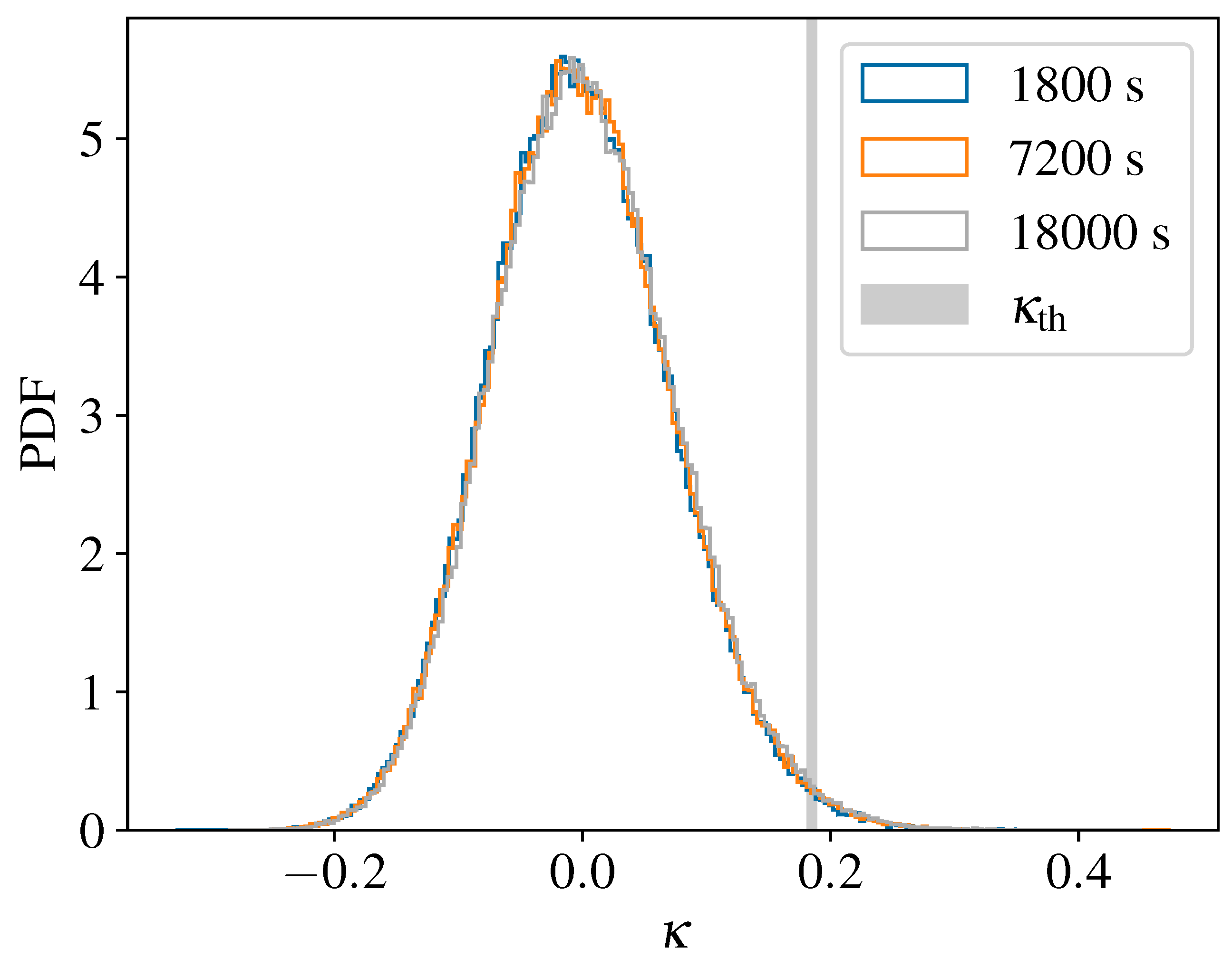
2.1. Expected Kurtosis from a Finite Gaussian Sample

Several kurtosis estimators have been proposed in the literature [43,44]. The distribution of these estimators is generally dependent on the distribution of the underlying samples, and must be characterized in order to cogently quantify deviations from Gaussianity. In this work, we compute the sample kurtosis using the scipy.stats.kurtosis function as implemented in SciPy [45]. To characterize kurtosis distribution, shown in Figure 2, we numerically generate 1.6 × 10 5 noise power spectra and compute the sample kurtosis.
Samples are generated using lalpulsar_Makefakedata_v5 [46] to simulate a 1-year Gaussian-noise datastream with a PSD of S n = 1 × 10 46 Hz 1 . SFTs were generated using three different time lengths, namely T SFT = 1800 s , 7200 s , 18,000 s. For each SFT, we computed their power spectrum [Equation (7)], which was then used to compute the sample’s kurtosis κ . The frequency band Δ f was adjusted according to T SFT so that all samples contained Δ f / δ f = 4500 frequency bins; as a result, sample kurtosis is always estimated using the same number of samples and thus the kurtosis distributions for all T SFT values are comparable.
Figure 1. (Top) Power spectra for the three CW signals at f 0 = 50 Hz and null spindown parameter. (Bottom) Distribution of power spectra and kurtosis for the three same CW signals. As discussed in Section 1, the width of the spectral artifact is related to the sky position of the CW source. Sources away from the sky poles (low declination δ 1 ) tend to produce broader signals than sources closer to the sky poles (high declination δ 1.5 ), The amplitudes of these signals correspond to a sensitivity depth of D = 15 for illustration purposes. We refer the reader to Section 2.2 and Section 3 for a detailed discussion on relevant CW amplitudes.
Universe 10 00121 g001
We select a kurtosis threshold κ th corresponding to the 99% quantile of the resulting kurtosis distribution for each T SFT , as shown in Table 1. Any Gaussian-noise power spectrum yielding a kurtosis above κ th will be flagged as containing a visible CW signal. We exemplify this visibility criterion in Figure 3, where we show a “visible’” CW signal according to our criterion κ > κ th .
Figure 2. Distribution of sample kurtosis using 1.6 × 10 5 Gaussian noise realizations for T SFT = 1800 s , 7200 s , 18,000 s. Each realization lasts for 1 year and contains 4500 frequency bins. Thresholds corresponding to the 99% quantile are highlighted in gray and collected in Table 1.
Universe 10 00121 g002
This criterion will be used in Section 2.2 to compute the visible fraction of an astrophysically motivated population of CW sources. Concretely, we will compute the CW amplitude at which a certain fraction of the population of CW signals returns a kurtosis above κ th . The choice of κ th as the 99% quantile implies that the amplitudes corresponding to small visible fractions (e.g., less than 10% of visible signals) will be slightly overestimated, as 1% of the strictly non-visible signals will pass the threshold due to noise fluctuations. The results here reported, will therefore be conservative in the sense that the risks associated to a CW signal being visible in the power spectrum will not be underestimated.

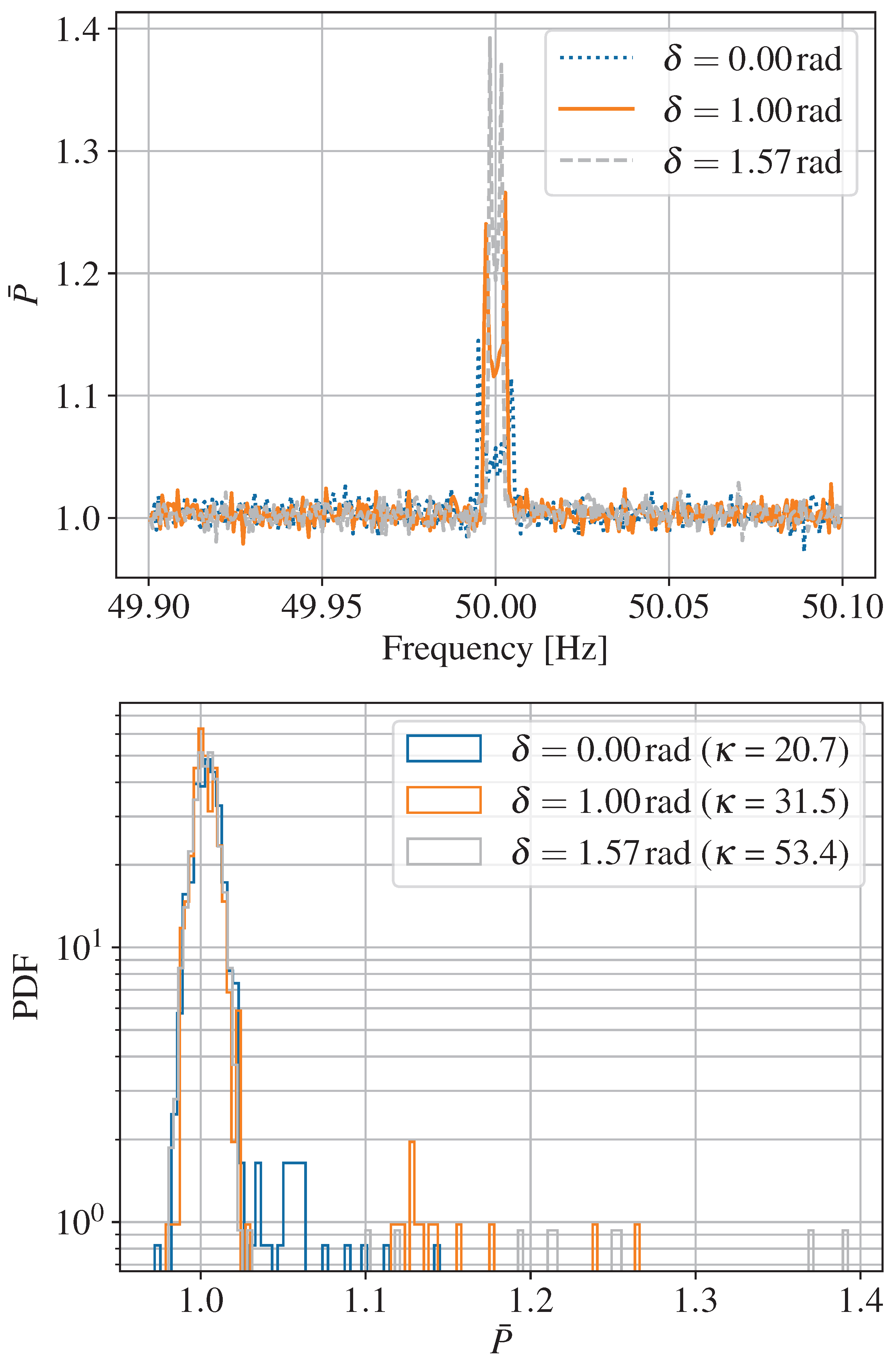
2.2. Kurtosis from CW Signals

To characterize the visibility of CW signals in a power spectrum, we simulate a population of CW sources with different amplitudes and determine the fraction of signals above the kurtosis threshold κ th computed in Section 2.1. We then compute, using a numerical fit, the amplitude at which a representative fraction of signals is found.This process is akin to sensitivity estimation procedures used in CW searches (e.g., [47] and references therein).
We simulate a population of all-sky isotropically oriented sources. This corresponds to sampling the sky-position angles ( α , δ ) from a uniform distribution on the sky sphere, and uniformly sampling the polarisation angle ψ π / 4 , π / 4 , the cosine of the inclination angle cos ι 1 , 1 , and the initial phase ϕ 0 0 , 2 π .
We select eight representative frequency bands across the frequency range expected for a CW signal, namely 10 , 30 , 100 , 200 , 300 , 500 , 700 , 1000 Hz }. This choice is motivated by the fact that the bandwidth of the Doppler modulations induced on the CW are proportional to the CW’s frequency [Equation (2)]: higher frequencies are expected to modulate along broader frequency bands, and thus produce less prominent peaks than lower frequencies.
For simplicity, we set all the spindown parameters to zero. This is consistent with the usual spindown values observed in the known pulsar population [48]. Non-zero spindown values may cause a broader modulation of the CW’s frequency, which in turn may diminish the prominence of the resulting peak in the power spectrum, reducing the visibility of a signal. This choice is in line with producing a conservative result that does not underestimate the visibility of a CW signal in the power spectrum.
The CW amplitude h 0 is specified in terms of the sensitivity depth D [2,49,50]
D = S n Hz h 0 .
We select a range of sensitivity depth values from 0.1 to 80 in order to sample the full range of visibility fractions. PSD is fixed to S n = 1 × 10 46 Hz 1 .
Throughout this analysis, we simulate signals as seen in a 1-year observing run of the Advanced LIGO Hanford detector. Since (1) the duration of the observing run is on the order of a year, (2) CW sources are uniformly distributed across the sky, (3) CW signals span a very narrow frequency band, in the sense that the PSD can be considered constant, and (4) amplitudes are expressed relative to PSD by means of the sensitivity depth, the resulting sensitivity depths are valid for any other ground-based interferometric detector, and will be used in Section 2.2 to estimate the visibility of a possible astrophysical population of CW sources for different detectors.
For each depth and frequency band, we simulate N I = 3000 CW signals in Gaussian noise and compute the fraction of visible signals p V ( D ) as
p V ( D ) = 1 N I n = 1 N I 1 , if κ ( n ) > κ th 0 , otherwise ,
where κ ( n ) is the kurtosis of the n-th simulated signal. This quantity describes the fraction of visible signals in a population with a given constant depth. More generally, p V is the probability of drawing a visible signal from the specified population at a given depth. The results are shown in Figure 4.
The specific p V value of interest depends on the application at hand. We fit a sigmoid-like ansatz using the function NonlinearModelFit as implemented in Mathematica [51] to p V
p V ( D ; a , b ) = 1 1 + b D 5 / 2 e a / D
and compute the visible sensitivity depth at p V = 10 % and p V = 90 % .
The resulting sensitivity depths are listed in Table 2 and shown in Figure 5, and follow the expected trend: higher frequencies produce a broader Doppler modulation, and thus require a higher amplitude (lower depth) in order to produce a visible peak in the power spectrum. The higher the p V , the bigger the fraction of visible signals; as a result, at a given frequency, D tends to decrease (higher amplitudes) as we increase p V . As discussed in Table 2, the results appear to be shifted for different T SFT values. This is a result of the different kurtosis thresholds, as discussed in Table 1. From Figure 5, we can conclude that low-frequency CW signals tend to be “more visible” than high-frequency signals at a similar amplitude, in the sense that the lower Doppler modulation allows for a more prominent peak to be displayed.
These sensitivity depths should be interpreted as the relative amplitude with respect to the background noise required for a CW signal to be visible in a power spectrum. For a given detector PSD, these values can be converted to the corresponding CW amplitude h 0 using Equation (11). To understand the risks associated to a visible CW signal, such as mistakenly flagging it as an unknown line or whether visible artifacts are enough to ascribe a non-astrophysical origin, however, we should compare these results to the expected amplitude from a population of astrophysical CW sources.

3. Implications for Astrophysical CW Sources

The visible sensitivity depths recorded in Table 2 must be compared to a realistic estimate of the expected amplitude of a CW signal in order to assess the risks associated to a visible CW signal in the power spectrum. Since no CW signal has been detected to date, we will follow the conservative approach taken so far and construct an optimistic astrophysical CW source (Section 3.1) to compare against the obtained results for different detector configurations (Section 3.2).

3.1. An Optimistic CW Source

The nominal amplitude of a CW signal h 0 emitted by a NS with a quadrupolar deformation parametrized by the equatorial ellipticity ε is given by [13]
h 0 = 4 π 2 G c 4 I f 0 2 ε d ,
where f 0 is the CW frequency (twice the rotational frequency in this model), d is the distance from the NS to the detector, and I = 10 38 kg m 2 is the canonical moment of inertia of an NS around the spinning axis [52]2. The results from this section could also be re-interpreted assuming other other emission mechanisms, such as r-modes or free precession [2,53].
The latests theoretical bounds on the maximum ellipticity sustained by a NS are ε 10 6 [54,55]. This upper bound increases by a few orders of magnitude if more exotic objects are considered [56]. On the lower end, the observed population of millisecond pulsars appears to sustain an ellipticity of about ε 10 9 [57].
We construct an optimistic CW source by considering the full range of plausible ellipticities ε [ 10 9 , 10 6 ] for a NS located at d = 20 pc , which corresponds to the closest location to the detector at which an NS is expected to be found [58]. Note that h 0 depends on the ratio ε / d ; for example, the expected amplitude of a source with ε = 10 6 at 2 kpc is equal to that of a source with ε = 10 8 at 20 pc . In Figure 6, we show the expected sensitivity depth for optimistic sources in the sensitive band of the Advanced LIGO (O3, O4, and O5 sensitivities) [59,60,61,62], Einstein Telescope [63,64], and Cosmic Explorer [65] detectors. This is computed by using Equation (14) and the available PSD curves in the literature.
The resulting sensitivity depth curves are such that D S n f 0 2 . For a given ellipticity and distance to the source, low frequencies tend to produce high depth values (weak signals) as h 0 f 0 2 and the PSD of the detector tends ot be very steep. Toward higher frequencies, where shot-noise is dominant, h 0 grows faster than the detector’s PSD, resulting in a monotonically decreasing sensitivity depth (increasing signal amplitude). For a given ellipticity and distance to the source, a CW signal is “easier” to detect at a high frequency than at a low frequency.
We note that all-sky CW search upper limits in O3 data [47] rule out this optimistic population. Said upper limits, however, are only valid for deterministic CW signals whose frequency evolution is not affected by stochastic effects, such as glitches [66,67] or spin-wandering [68]. For a generic CW signal, the results as reported by the SOAP pipeline [69,70] are less constraining.

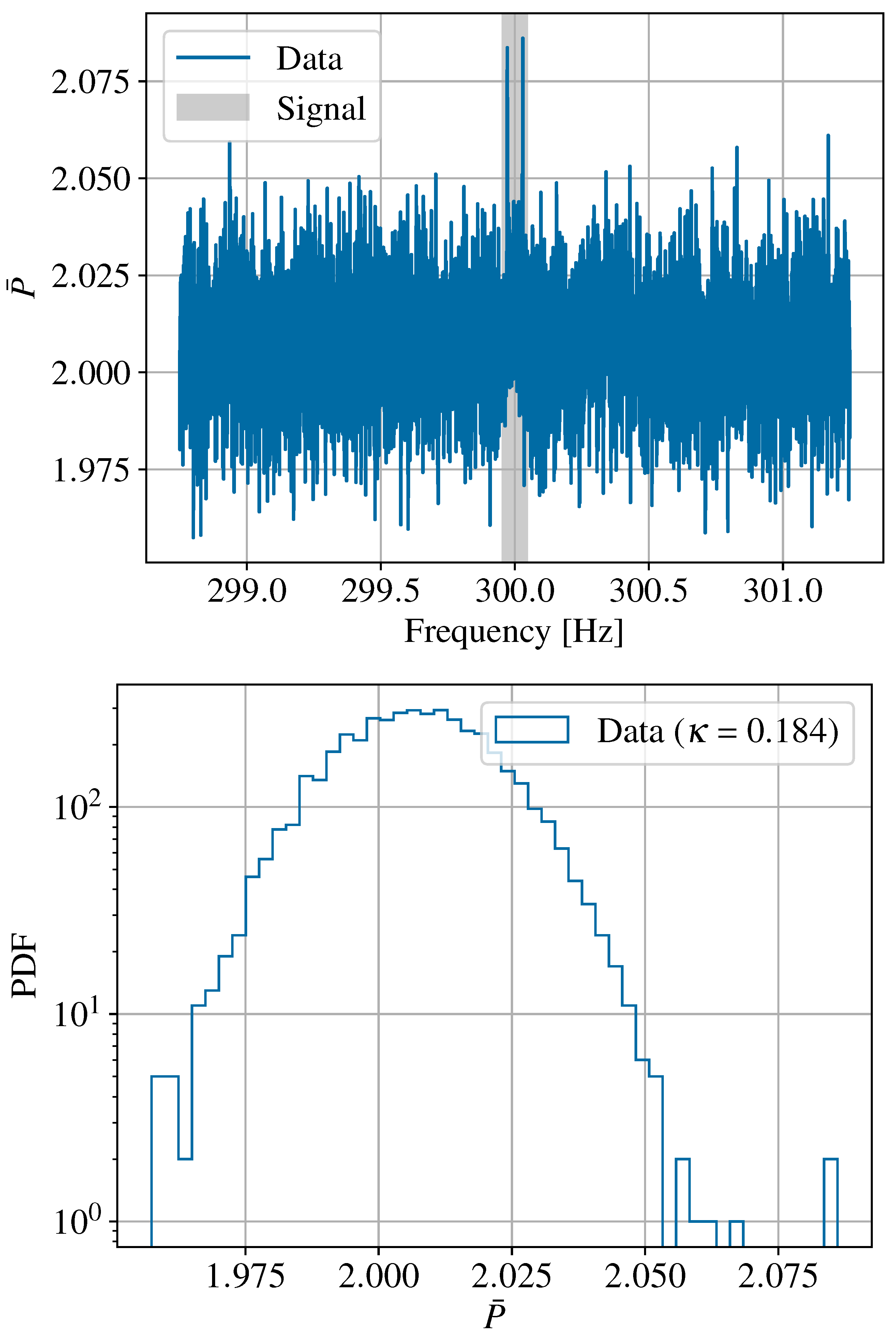
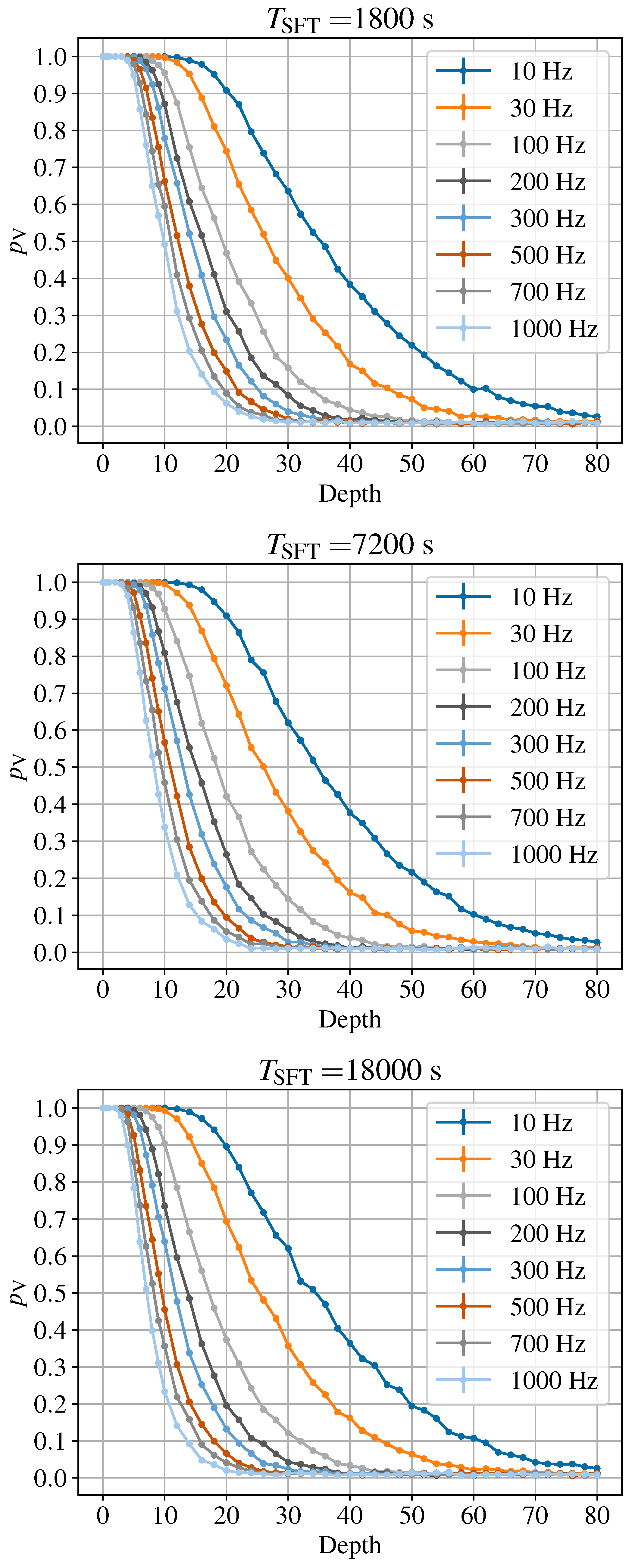
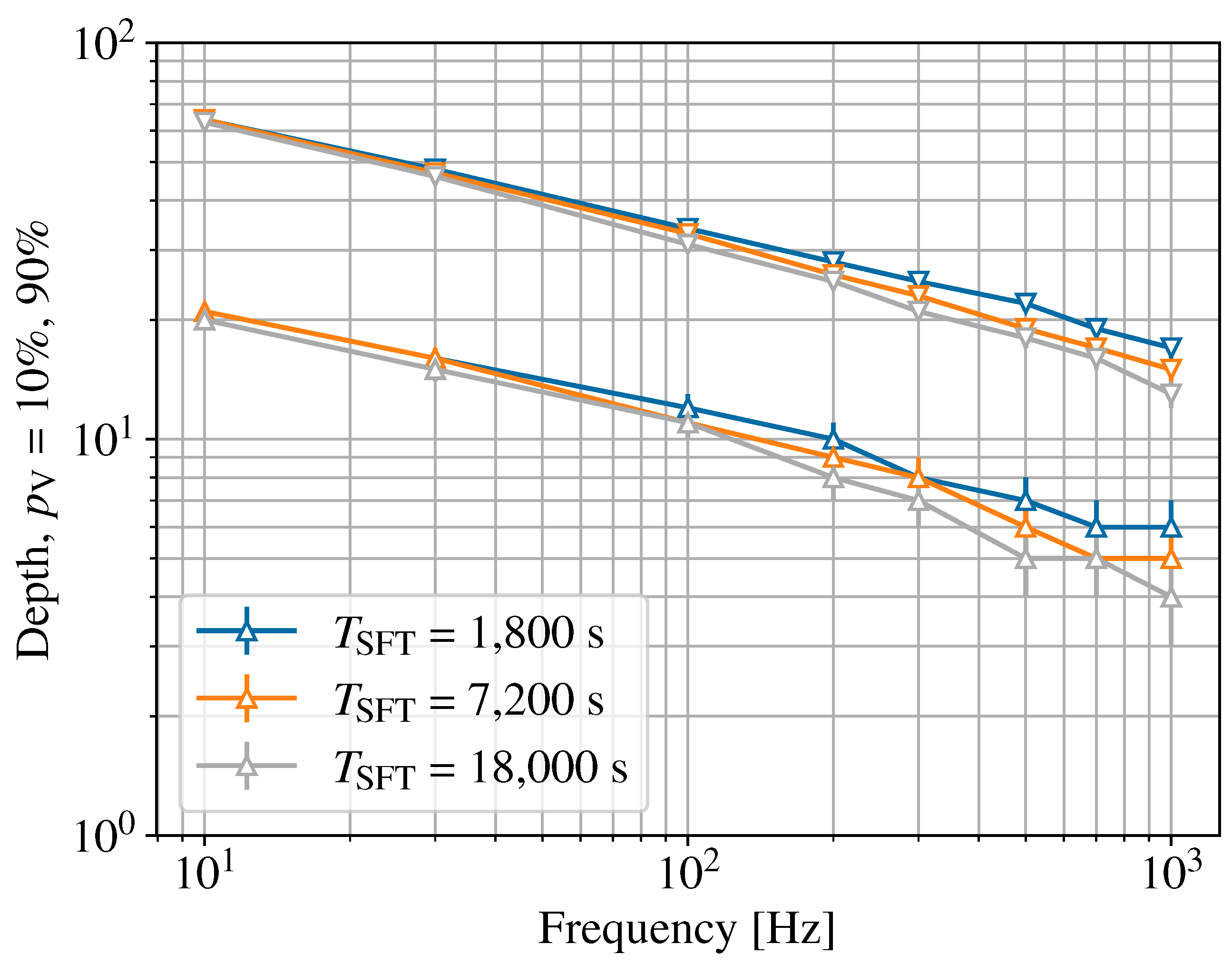
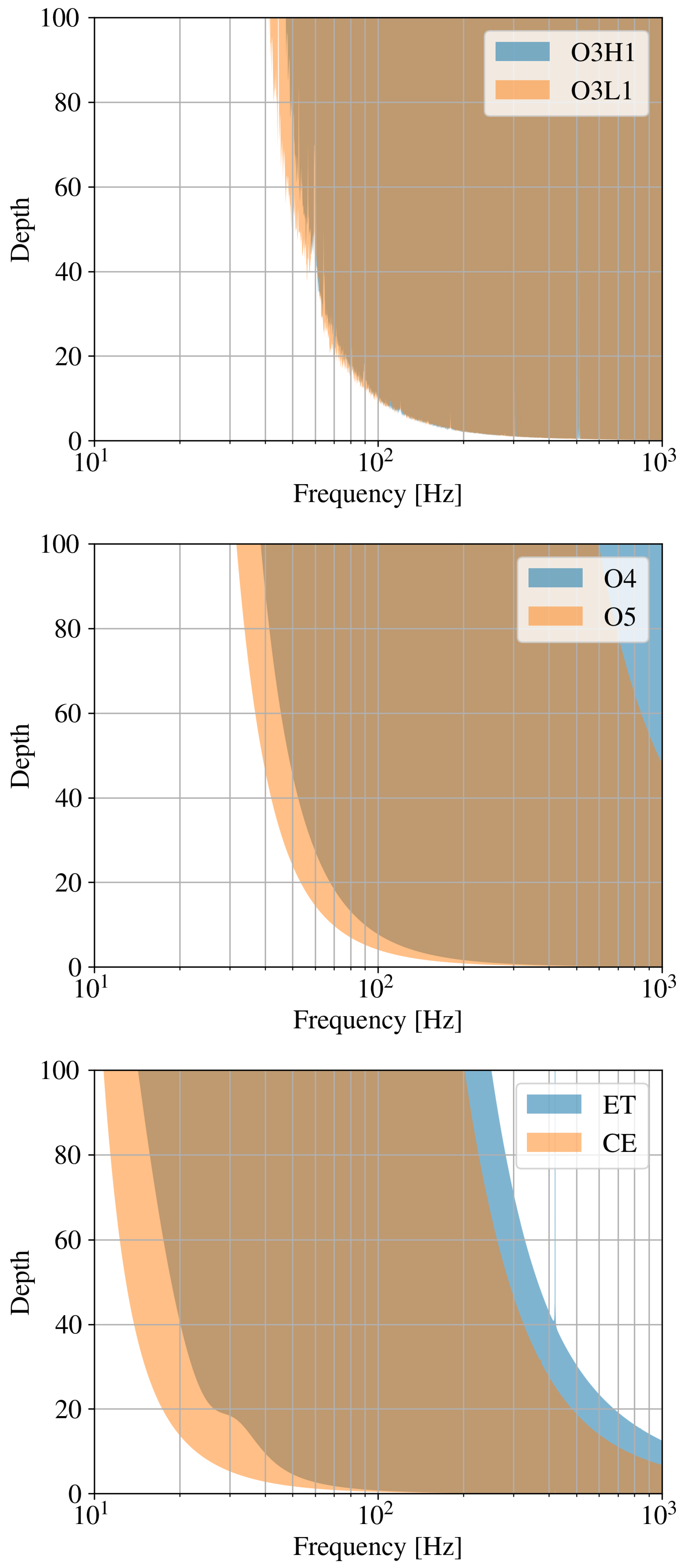
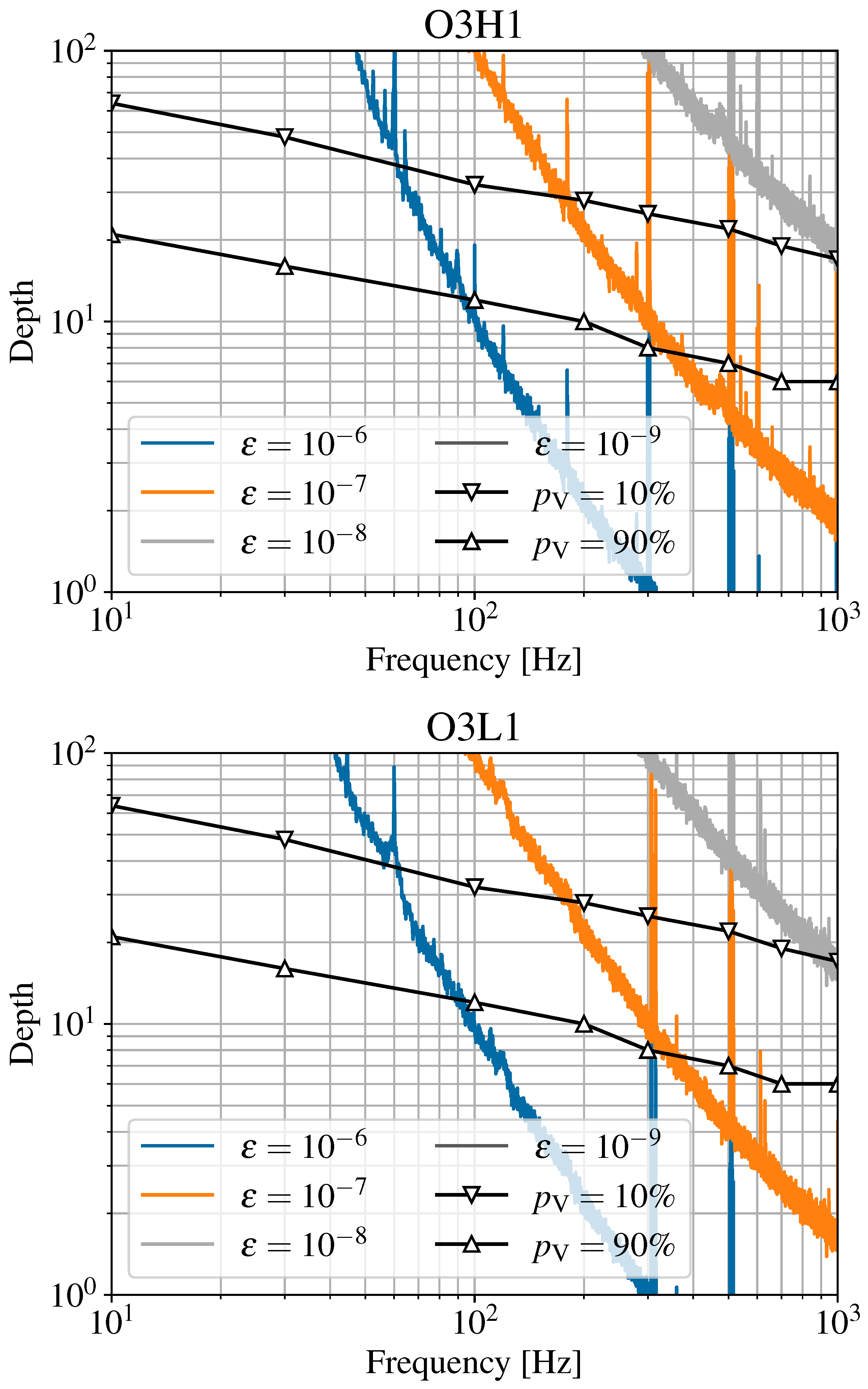
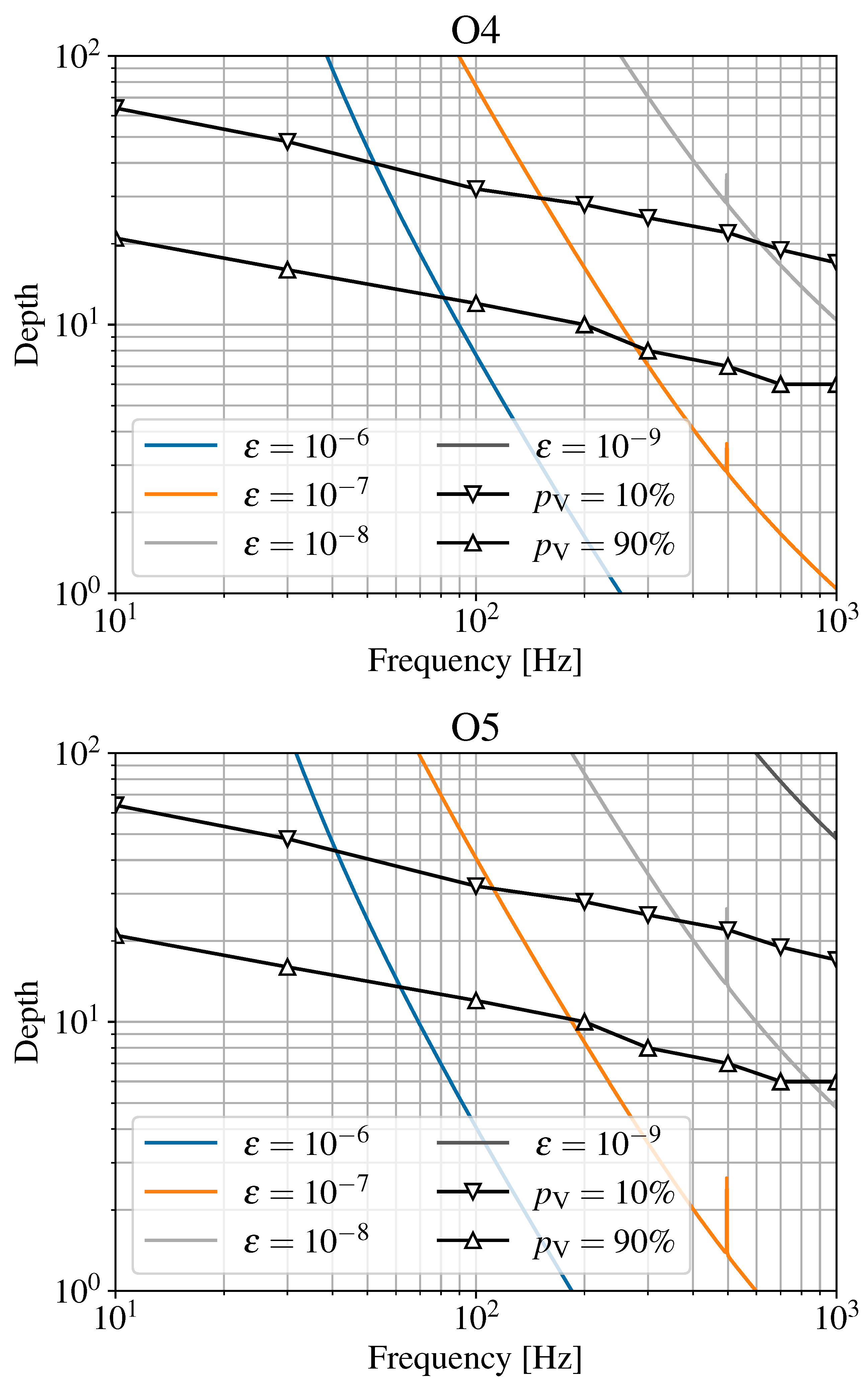
3.2. Visibility of CW Signals in a Power Spectra

In Figure 7, Figure 8 and Figure 9, we compare the visible sensitivity depths derived in Section 2 to the expected sensitivity depths from astrophysical CW signals introduced in Section 3.1. To ease the discussion, we use the results using T SFT = 1800 s , which are the most conservative. Other T SFT values produce comparable results as the variations are small.
We are interested in identifying frequency bands for which the visible sensitivity depth is higher than the expected depth for an optimistic CW signal. In such bands, CW signals will be visible in the power spectrum.
Overall, we find that visible signals tend to be located in the upper end of the frequency spectrum. This fact seems to contradict the results from Section 2.2, where we concluded that high frequencies are less visible than low frequencies due to a broader Doppler modulation. The detector’s sensitivity curve, however, degrades very steeply towards low frequencies; towards high frequencies, where shot-noise is dominant, the frequency dependence is much more gentle compared to h 0 ’s quadratic dependency on f 0 , and thus the resulting sensitivity depth rapidly becomes lower enough to be visible.
For high ellipticity values, ε 10 7 , 10 6 , and for the Advanced LIGO detectors in their O3 configuration (Figure 7), CW signals may start to become visible at about 100 Hz . As we progress into O4 and O5 sensitivities (Figure 8), this frequency may reduce close to 50 Hz . Typical searches for CW signals from unknown sources survey frequencies within [ 20 , 1000 ] Hz [47]. As a result, as we approach the design sensitivity of the Advanced detectors, CW signals are expected to be visible for 95 % of the frequency band. For 3G detectors (Figure 9), high ellipticity signals will be visible across practically the whole frequency band.
For low ellipticities ε 10 9 , 10 8 , CW signals may become visible starting at 700 Hz during O4 and 500 Hz during O5. For 3G detectors, low ellipticity signals may be visible from 100 Hz onward.

4. Conclusions

We have studied whether an astrophysical CW signal could be visible as a narrow spectral artifact in the power spectrum of a gravitational-wave detector. To do so, we have calibrated the sample kurtosis of a power spectrum as a measure of the visibility of a CW signal. We found that, depending on the signal’s frequency, sensitivity depths between D = 5 and D = 60 could become visible in a power spectrum, and thus mimic the behavior of a line.
These results were compared to the expected amplitude of an optimistic astrophysical signal. For high ellipticities ε 10 7 , 10 6 , CW signals become visible from 100 Hz onward for the Advanced LIGO detectors which amount to 95% of the frequency bands surveyed in a typical all-sky search; for 3G detectors, signals will be visible across the whole frequency band. For low ellipticities ε 10 9 , 10 8 , CW signals may start to become visible at 700 Hz for the O4 detectors, 500 Hz for the O5 detectors, and 100 Hz for the 3G detectors. We conclude that it is unsafe to discard CW search outliers near narrow spectral artifacts of unknown origin. Safely discarding outliers near spectral artifacts requires evidence that the artifact is instrumental.
Throughout this study, we assumed a population of CW signals with a negligible spindown parameter f 1 0 Hz / s . Given the typical resolution of an all-sky CW search, this assumption is consistent with the observed pulsar population [48]. The impact of higher spindown values may be to spread the power of a CW signal along neighboring frequency bins, reducing the peak’s prominence in a power spectrogram. This is more likely to affect high ellipticity sources, which are expected to have a higher spindown value. The results here presented tend to overestimate the visibility of high ellipticity sources.
Also, in this study we neglected two properties of CW signals, namely their distinctive double-horned shape in a power spectrum [34] and the fact that they may be expected to show up in multiple detectors at once. The former requires the CW signal to be located in a relatively quiet frequency band, as otherwise the expected horns would end up tarnished by instrumental or unknown lines. The latter requires a network of detectors with comparable sensitivities at a given frequency band, which makes it depend heavily on the specific configuration of the detectors.
Our results draw attention to the importance of conducting detector characterization studies on narrow spectral artifacts, and to the non-negligible possibility of missing an obvious CW signal if such tasks are neglected. Although a significant (and increasing) number of lines have been characterized and mitigated thanks to detector characterization efforts within the LIGO–Virgo–KAGRA collaboration, the origin of a comparable amount still remains, to date, unknown. The importance of rigorous investigation to distinguish between instrumental artifacts and genuine CW signals will only increase as we progress into the era of design sensitivity of the advanced detectors and further beyond into 3G.

Author Contributions

All authors contributed equally. All authors have read and agreed to the published version of the manuscript.

Funding

This work was supported by the Universitat de les Illes Balears (UIB); the Spanish Agencia Estatal de Investigación grants PID2022-138626NB-I00, PID2019-106416GB-I00, RED2022-134204-E, RED2022- 134411-T, funded by MCIN/AEI/10.13039/501100011033; the MCIN with funding from the European Union NextGenerationEU/PRTR (PRTR-C17.I1); Comunitat Autònoma de les Illes Balears through the Direcció General de Recerca, Innovació I Transformació Digital with funds from the Tourist Stay Tax Law (PDR2020/11—ITS2017-006), the Conselleria d’Economia, Hisenda i Innovació co-financed by the European Union and FEDER Operational Program 2021–2027 of the Balearic Islands; the “ERDF A way of making Europe”. R.J. is supported by the Conselleria de Educació, Universitat i Recerca del Govern de les Illes Balears FPI/018/2020.

Data Availability Statement

All the data used in this article is already included in the article.

Acknowledgments

We thank Ansel Neunzert, Evan Goetz, David Keitel, and the Continuous Wave working group of the LIGO–Virgo–KAGRA Collaboration for useful comments and discussions. This paper has been assigned document number LIGO-P2300463.

Conflicts of Interest

The authors declare no conflicts of interest.

Notes

1
A notable exception are the Einstein@Home CW searches (see [31] and references therein), which use a detection statistic that extends the noise hypothesis to include lines [32].
2
As discussed in [52], the moment of inertia differs by a factor of ∼3 for different equations of state. Conversely, as discussed in the text, the equatorial ellipticity has a broader dynamical range depending on the sourcing mechanism; as a result, we choose to fix the moment of inertia to the canonical value and focus our discussion on ε .

References

  1. Riles, K. Searches for continuous-wave gravitational radiation. Living Rev. Rel. 2023, 26, 3. [Google Scholar] [CrossRef]
  2. Wette, K. Searches for continuous gravitational waves from neutron stars: A twenty-year retrospective. Astropart. Phys. 2023, 153, 102880. [Google Scholar] [CrossRef]
  3. Sieniawska, M.; Bejger, M. Continuous gravitational waves from neutron stars: Current status and prospects. Universe 2019, 5, 217. [Google Scholar] [CrossRef]
  4. Zhu, S.J.; Baryakhtar, M.; Papa, M.A.; Tsuna, D.; Kawanaka, N.; Eggenstein, H.B. Characterizing the continuous gravitational-wave signal from boson clouds around Galactic isolated black holes. Phys. Rev. D 2020, 102, 063020. [Google Scholar] [CrossRef]
  5. Jones, D.; Sun, L.; Siemonsen, N.; East, W.E.; Scott, S.M.; Wette, K. Methods and prospects for gravitational-wave searches targeting ultralight vector-boson clouds around known black holes. Phys. Rev. D 2023, 108, 064001. [Google Scholar] [CrossRef]
  6. Miller, A.L.; Clesse, S.; De Lillo, F.; Bruno, G.; Depasse, A.; Tanasijczuk, A. Probing planetary-mass primordial black holes with continuous gravitational waves. Phys. Dark Univ. 2021, 32, 100836. [Google Scholar] [CrossRef]
  7. Miller, A.L.; Aggarwal, N.; Clesse, S.; De Lillo, F. Constraints on planetary and asteroid-mass primordial black holes from continuous gravitational-wave searches. Phys. Rev. D 2022, 105, 062008. [Google Scholar] [CrossRef]
  8. Aasi, J.; Abbott, B.P.; Abbott, R.; Abbott, T.; Abernathy, M.R.; Ackley, K.; Adams, C.; Adams, T.; Addesso, P.; Adhikari, R.X.; et al. Advanced LIGO. Class. Quant. Grav. 2015, 32, 074001. [Google Scholar] [CrossRef]
  9. Acernese, F.A.; Agathos, M.; Agatsuma, K.; Aisa, D.; Allemandou, N.; Allocca, A.; Amarni, J.; Astone, P.; Balestri, G.; Ballardin, G.; et al. Advanced Virgo: A second-generation interferometric gravitational wave detector. Class. Quant. Grav. 2015, 32, 024001. [Google Scholar] [CrossRef]
  10. Akutsu, T.; Ando, M.; Arai, K.; Arai, Y.; Araki, S.; Araya, A.; Aritomi, N.; Asada, H.; Aso, Y.; Atsuta, S.; et al. KAGRA: 2.5 Generation Interferometric Gravitational Wave Detector. Nat. Astron. 2019, 3, 35–40. [Google Scholar] [CrossRef]
  11. Maggiore, M.; Van Den Broeck, C.; Bartolo, N.; Belgacem, E.; Bertacca, D.; Bizouard, M.A.; Branchesi, M.; Clesse, S.; Foffa, S.; García-Bellido, J.; et al. Science Case for the Einstein Telescope. JCAP 2020, 03, 050. [Google Scholar] [CrossRef]
  12. Reitze, D.; Adhikari, R.X.; Ballmer, S.; Barish, B.; Barsotti, L.; Billingsley, G.; Brown, D.A.; Chen, Y.; Coyne, D.; Eisenstein, R.; et al. Contribution to Gravitational-Wave Astronomy beyond LIGO. Bull. Am. Astron. Soc. 2019, 51, 035. [Google Scholar]
  13. Jaranowski, P.; Krolak, A.; Schutz, B.F. Data analysis of gravitational-wave signals from spinning neutron stars. 1. The Signal and its detection. Phys. Rev. D 1998, 58, 063001. [Google Scholar] [CrossRef]
  14. Krishnan, B.; Sintes, A.M.; Papa, M.A.; Schutz, B.F.; Frasca, S.; Palomba, C. The Hough transform search for continuous gravitational waves. Phys. Rev. D 2004, 70, 082001. [Google Scholar] [CrossRef]
  15. Knispel, B.; Allen, B. Blandford’s Argument: The Strongest Continuous Gravitational Wave Signal. Phys. Rev. D 2008, 78, 044031. [Google Scholar] [CrossRef]
  16. Wade, L.; Siemens, X.; Kaplan, D.L.; Knispel, B.; Allen, B. Continuous Gravitational Waves from Isolated Galactic Neutron Stars in the Advanced Detector Era. Phys. Rev. D 2012, 86, 124011. [Google Scholar] [CrossRef]
  17. Tenorio, R.; Keitel, D.; Sintes, A.M. Search Methods for Continuous Gravitational-Wave Signals from Unknown Sources in the Advanced-Detector Era. Universe 2021, 7, 474. [Google Scholar] [CrossRef]
  18. Sarin, N.; Lasky, P.D.; Sammut, L.; Ashton, G. X-ray guided gravitational-wave search for binary neutron star merger remnants. Phys. Rev. D 2018, 98, 043011. [Google Scholar] [CrossRef]
  19. Oliver, M.; Keitel, D.; Sintes, A.M. Adaptive transient Hough method for long-duration gravitational wave transients. Phys. Rev. D 2019, 99, 104067. [Google Scholar] [CrossRef]
  20. Grace, B.; Wette, K.; Scott, S.M.; Sun, L. Piecewise frequency model for searches for long-transient gravitational waves from young neutron stars. Phys. Rev. D 2023, 108, 123045. [Google Scholar] [CrossRef]
  21. Prix, R.; Itoh, Y. Global parameter-space correlations of coherent searches for continuous gravitational waves. Class. Quant. Grav. 2005, 22, S1003–S1012. [Google Scholar] [CrossRef]
  22. Leaci, P. Methods to filter out spurious disturbances in continuous-wave searches from gravitational-wave detectors. Phys. Scr. 2015, 90, 125001. [Google Scholar] [CrossRef]
  23. Berger, B.K. Identification and mitigation of Advanced LIGO noise sources. J. Phys. Conf. Ser. 2018, 957, 012004. [Google Scholar] [CrossRef]
  24. Cabero, M.; Lundgren, A.; Nitz, A.H.; Dent, T.; Barker, D.; Goetz, E.; Kissel, J.S.; Nuttall, L.K.; Schale, P.; Schofield, R.; et al. Blip glitches in Advanced LIGO data. Class. Quant. Grav. 2019, 36, 15. [Google Scholar] [CrossRef]
  25. Davis, D.; Areeda, J.S.; Berger, B.K.; Bruntz, R.; Effler, A.; Essick, R.C.; Fisher, R.P.; Godwin, P.; Goetz, E.; Helmling-Cornell, A.F.; et al. LIGO detector characterization in the second and third observing runs. Class. Quant. Grav. 2021, 38, 135014. [Google Scholar] [CrossRef]
  26. Vazsonyi, L.; Davis, D. Identifying glitches near gravitational-wave signals from compact binary coalescences using the Q-transform. Class. Quant. Grav. 2023, 40, 035008. [Google Scholar] [CrossRef]
  27. Davis, D.; Littenberg, T.B.; Romero-Shaw, I.M.; Millhouse, M.; McIver, J.; Di Renzo, F.; Ashton, G. Subtracting glitches from gravitational-wave detector data during the third LIGO-Virgo observing run. Class. Quant. Grav. 2022, 39, 245013. [Google Scholar] [CrossRef]
  28. Covas, P.B.; Effler, A.; Goetz, E.; Meyers, P.M.; Neunzert, A.; Oliver, M.; Pearlstone, B.L.; Roma, V.J.; Schofield, R.M.S.; Adya, V.B.; et al. Identification and mitigation of narrow spectral artifacts that degrade searches for persistent gravitational waves in the first two observing runs of Advanced LIGO. Phys. Rev. D 2018, 97, 082002. [Google Scholar] [CrossRef]
  29. Goetz, E.; Neunzert, A.; Riles, K.; Matas, A.; Kandhasamy, S.; Tasson, J.; Barschaw, C.; Middleton, H.; Hughey, S.; Mueller, L.; et al. O3 Lines and Combs in Found in Self-Gated C01 Data. 2021. Available online: https://dcc.ligo.org/LIGO-T2100200/public (accessed on 1 December 2023).
  30. Goetz, E.; Neunzert, A.; Riles, K.; Matas, A.; Kandhasamy, S.; Tasson, J.; Barschaw, C.; Middleton, H.; Hughey, S.; Mueller, L.; et al. Unidentified O3 Lines Found in Self-Gated C01 Data. 2021. Available online: https://dcc.ligo.org/LIGO-T2100201/public (accessed on 1 December 2023).
  31. Steltner, B.; Papa, M.A.; Eggenstein, H.B.; Prix, R.; Bensch, M.; Allen, B.; Machenschalk, B. Deep Einstein@Home All-sky Search for Continuous Gravitational Waves in LIGO O3 Public Data. Astrophys. J. 2023, 952, 55. [Google Scholar] [CrossRef]
  32. Keitel, D.; Prix, R.; Papa, M.A.; Leaci, P.; Siddiqi, M. Search for continuous gravitational waves: Improving robustness versus instrumental artifacts. Phys. Rev. D 2014, 89, 064023. [Google Scholar] [CrossRef]
  33. Zhu, S.J.; Papa, M.A.; Walsh, S. New veto for continuous gravitational wave searches. Phys. Rev. D 2017, 96, 124007. [Google Scholar] [CrossRef]
  34. Valluri, S.R.; Dergachev, V.; Zhang, X.; Chishtie, F.A. Fourier transform of the continuous gravitational wave signal. Phys. Rev. D 2021, 104, 024065. [Google Scholar] [CrossRef]
  35. Tenorio, R.; Keitel, D.; Sintes, A.M. Application of a hierarchical MCMC follow-up to Advanced LIGO continuous gravitational-wave candidates. Phys. Rev. D 2021, 104, 084012. [Google Scholar] [CrossRef]
  36. Jones, D.; Sun, L.; Carlin, J.; Dunn, L.; Millhouse, M.; Middleton, H.; Meyers, P.; Clearwater, P.; Beniwal, D.; Strang, L.; et al. Validating continuous gravitational-wave candidates from a semicoherent search using Doppler modulation and an effective point spread function. Phys. Rev. D 2022, 106, 123011. [Google Scholar] [CrossRef]
  37. Allen, B.; Goetz, E.; Keitel, D.; Landry, M.; Mendell, G.; Prix, R.; Riles, K.; Wette, K. SFT Data Format Version 2–3 Specification. 2023. Available online: https://dcc.ligo.org/LIGO-T040164 (accessed on 1 December 2023).
  38. Bretthorst, G.L. Bayesian Spectrum Analysis and Parameter Estimation; Springer: New York, NY, USA, 1988. [Google Scholar] [CrossRef]
  39. Das, K. A Brief Review of Tests for Normality. Am. J. Theor. Appl. Stat. 2016, 5, 5. [Google Scholar] [CrossRef]
  40. Owen, B.J.; Lindblom, L.; Pinheiro, L.S.; Rajbhandari, B. Improved Upper Limits on Gravitational Wave Emission from NS 1987A in SNR 1987A. Astrophys. J. Lett. 2023, 962, L23. [Google Scholar] [CrossRef]
  41. Cramér, H. On the composition of elementary errors. Scand. Actuar. J. 1928, 1928, 13–74. [Google Scholar] [CrossRef]
  42. Westfall, P.H. Kurtosis as Peakedness, 1905–2014. R.I.P. Am. Stat. 2014, 68, 191–195. [Google Scholar] [CrossRef] [PubMed]
  43. Joanes, D.N.; Gill, C.A. Comparing measures of sample skewness and kurtosis. J. R. Stat. Soc. Ser. (The Stat.) 1998, 47, 183–189. [Google Scholar] [CrossRef]
  44. Fisher, R.A. The Moments of the Distribution for Normal Samples of Measures of Departure from Normality. Proc. R. Soc. Lond. Ser. A 1930, 130, 16–28. [Google Scholar] [CrossRef]
  45. Virtanen, P.; Gommers, R.; Oliphant, T.E.; Haberland, M.; Reddy, T.; Cournapeau, D.; Burovski, E.; Peterson, P.; Weckesser, W.; Bright, J.; et al. SciPy 1.0: Fundamental Algorithms for Scientific Computing in Python. Nat. Methods 2020, 17, 261–272. [Google Scholar] [CrossRef] [PubMed]
  46. LIGO Scientific Collaboration; Virgo Collaboration; KAGRA Collaboration. LVK Algorithm Library—LALSuite. Free Software (GPL). Software Version 7.21. Available online: https://pypi.org/project/lalsuite/ (accessed on 1 December 2023).
  47. Abbott, R.; Abe, H.; Acernese, F.; Ackley, K.; Adhikari, N.; Adhikari, R.X.; Adkins, V.K.; Adya, V.B.; Affeldt, C.; Agarwal, D.; et al. All-sky search for continuous gravitational waves from isolated neutron stars using Advanced LIGO and Advanced Virgo O3 data. Phys. Rev. D 2022, 106, 102008. [Google Scholar] [CrossRef]
  48. Manchester, R.N.; Hobbs, G.B.; Teoh, A.; Hobbs, M. The Australia Telescope National Facility Pulsar Catalogue. Astrophys. J. 2005, 129, 1993–2006. [Google Scholar] [CrossRef]
  49. Behnke, B.; Papa, M.A.; Prix, R. Postprocessing methods used in the search for continuous gravitational-wave signals from the Galactic Center. Phys. Rev. D 2015, 91, 064007. [Google Scholar] [CrossRef]
  50. Dreissigacker, C.; Prix, R.; Wette, K. Fast and Accurate Sensitivity Estimation for Continuous-Gravitational-Wave Searches. Phys. Rev. D 2018, 98, 084058. [Google Scholar] [CrossRef]
  51. Wolfram Research, Inc. Mathematica, Version 13.3; Wolfram Research, Inc.: Champaign, IL, USA, 2023.
  52. Abbott, B.; Abbott, R.; Adhikari, R.; Agresti, J.; Ajith, P.; Allen, B.; Amin, R.; Anderson, S.B.; Anderson, W.G.; Arain, M.; et al. Upper limits on gravitational wave emission from 78 radio pulsars. Phys. Rev. D 2007, 76, 042001. [Google Scholar] [CrossRef]
  53. Tenorio, R. Blind-search constraints on the sub-kiloparsec population of continuous gravitational-wave sources. arXiv 2023, arXiv:2310.12097. [Google Scholar]
  54. Gittins, F.; Andersson, N. Modelling neutron star mountains in relativity. Mon. Not. Roy. Astron. Soc. 2021, 507, 116–128. [Google Scholar] [CrossRef]
  55. Morales, J.A.; Horowitz, C.J. Neutron star crust can support a large ellipticity. Mon. Not. Roy. Astron. Soc. 2022, 517, 5610–5616. [Google Scholar] [CrossRef]
  56. Owen, B.J. Maximum elastic deformations of compact stars with exotic equations of state. Phys. Rev. Lett. 2005, 95, 211101. [Google Scholar] [CrossRef]
  57. Woan, G.; Pitkin, M.D.; Haskell, B.; Jones, D.I.; Lasky, P.D. Evidence for a Minimum Ellipticity in Millisecond Pulsars. Astrophys. J. Lett. 2018, 863, L40. [Google Scholar] [CrossRef]
  58. Sartore, N.; Ripamonti, E.; Treves, A.; Turolla, R. Galactic neutron stars. I. Space and velocity distributions in the disk and in the halo. Astron. Astrophys. 2010, 510, A23. [Google Scholar] [CrossRef]
  59. Goetz, E. H1 Calibrated Sensitivity Spectra 4 January 2020 (Representative best of O3b – C01_CLEAN_SUB60HZ). 2021. Available online: https://dcc.ligo.org/LIGO-G2100674/public (accessed on 1 December 2023).
  60. Goetz, E. L1 Calibrated Sensitivity Spectra 4 January 2020 (Representative best of O3b – C01_CLEAN_SUB60HZ). 2021. Available online: https://dcc.ligo.org/LIGO-G2100675/public (accessed on 1 December 2023).
  61. Barsotti, L.; Fritschel, P.; Evans, M.; Gras, S. Updated Advanced LIGO Sensitivity Design Curve. 2018. Available online: https://dcc.ligo.org/LIGO-T1800044/public (accessed on 1 December 2023).
  62. Barsotti, L.; McCuller, L.; Evans, M.; Fritschel, P. Updated Advanced LIGO Sensitivity Design Curve. 2018. Available online: https://dcc.ligo.org/LIGO-T1800042/public (accessed on 1 December 2023).
  63. ET Design Study Team. ET-0001A-18/ET-0001A-18.txt. Available online: https://www.et-gw.eu/index.php/etsensitivities (accessed on 9 October 2023).
  64. Hild, S.; Chelkowski, S.; Freise, A.; Franc, J.; Morgado, N.; Flaminio, R.; DeSalvo, R. A Xylophone Configuration for a third Generation Gravitational Wave Detector. Class. Quant. Grav. 2010, 27, 015003. [Google Scholar] [CrossRef]
  65. Kuns, K.; Hall, E.; Srivastava, V.; Smith, J.; Evans, M.; Fritschel, P.; McCuller, L.; Wipf, C.; Ballmer, S. T2000017-v6/cosmic_explorer_strain.txt. Available online: https://dcc.cosmicexplorer.org/CE-T2000017/public (accessed on 9 October 2023).
  66. Ashton, G.; Prix, R.; Jones, D.I. Statistical characterization of pulsar glitches and their potential impact on searches for continuous gravitational waves. Phys. Rev. D 2017, 96, 063004. [Google Scholar] [CrossRef]
  67. Ashton, G.; Prix, R.; Jones, D.I. A semicoherent glitch-robust continuous-gravitational-wave search method. Phys. Rev. D 2018, 98, 063011. [Google Scholar] [CrossRef]
  68. Mukherjee, A.; Messenger, C.; Riles, K. Accretion-induced spin-wandering effects on the neutron star in Scorpius X-1: Implications for continuous gravitational wave searches. Phys. Rev. D 2018, 97, 043016. [Google Scholar] [CrossRef]
  69. Bayley, J.; Messenger, C.; Woan, G. Generalized application of the Viterbi algorithm to searches for continuous gravitational-wave signals. Phys. Rev. D 2019, 100, 023006. [Google Scholar] [CrossRef]
  70. Bayley, J.; Messenger, C.; Woan, G. Robust machine learning algorithm to search for continuous gravitational waves. Phys. Rev. D 2020, 102, 083024. [Google Scholar] [CrossRef]
Figure 3. Power spectrum of the Advanced LIGO Hanford detector containing a “visible” CW signal according to the kurtosis criterion κ > κ th . Data were generated using T SFT = 1800 s and S n = 1 × 10 46 Hz 1 . Signal parameters (see Section 2.2) are D = 9 , cos ι = 0.450 , α = 2.653 , δ = 0 , ϕ = 0.994 , ψ = 0.178 .
Universe 10 00121 g003
Figure 4. Fraction of visible signals p V for a population of all-sky isotropically oriented signals at different frequencies and sensitivity depths. Each simulated signal is injected in a 1-year dataset for the Advanced LIGO H1 detector. Each computed p V value has an associated binomial uncertainty of less than 1 % .
Universe 10 00121 g004
Figure 5. Sensitivity depth for p V = 10 % (downard triangles) and p V = 90 % (upward triangles) for different frequencies, as reported in Table 2.
Universe 10 00121 g005
Figure 6. Sensitivity depth for an optimistic CW source located at d = 20 pc for different ground-based interferometric detectors. The lower limit of the shaded area corresponds to ε = 10 6 ; the upper limit corresponds to ε = 10 9 . The presence of narrow artifacts in the O3 sensitivity depths is due to the use a PSD estimated using real data [59,60]. The shoulder-like plateau at low frequencies for the ET detector corresponds to the transition of the low-frequency interferometer to the high-frequency interferometer [64].
Universe 10 00121 g006
Figure 7. Expected sensitivity depth for an optimistic source consistent with a NS located at 20 pc as observed by the Advanced LIGO Hanford [59] (top) and Livingston [60] (bottom) detectors during O3. Solid lines correspond to different ellipticity values ( ε = 10 9 is beyond D = 100 ). Note that these are a discretized version of the shaded areas in Figure 6. Triangles correspond to visible sensitivity depths at p V = 10 % and p V = 90 % as reported in Table 2.
Universe 10 00121 g007
Figure 8. Same result as in Figure 7 for the Advanced LIGO detectors using the projected sensitivity for O4 [61] (top) and O5 [62] (bottom).
Universe 10 00121 g008
Figure 9. Same result as in Figure 7 for the projected third-generation detectors ET [63] (top) and CE [65] (bottom).
Universe 10 00121 g009
Table 1. Kurtosis thresholds corresponding to the 99% quantile of the numerically generated kurtosis distribution shown in Figure 2. We note that lower T SFT values tend to cause lower κ th . Since the duration of the observing run is fixed to 1 year, a lower T SFT value causes a higher number of SFTs to be generated. This causes the distribution of the resulting P ¯ to be closer to a Gaussian, which in turn diminishes the spread of the kurtosis distribution.
T SFT 1800 s7200 s18,000 s
κ th 0.1820.1850.188
Table 2. Sensitivity depth D for p V = 10 % and p V = 90 % as estimated from the results shown in Figure 4. The uncertainty in each value, which we estimated by propagating the binomial uncertainty on the empirical p V using the covariance matrix of the numerical fit, is ± 1 for all the values in the table. Depth values appear to be systematically biased toward higher values as we reduced T SFT . This is because κ th is lower for lower T SFT values, as discussed in Table 1.
T SFT p V 10 Hz30 Hz100 Hz200 Hz300 Hz500 Hz700 Hz1000 Hz
1800 s 90 % 211612108766
10 % 6448342825221917
7200 s 90 % 21161198655
10 % 6447332623191715
18,000 s 90 % 20151187554
10 % 6346312521181613
Disclaimer/Publisher’s Note: The statements, opinions and data contained in all publications are solely those of the individual author(s) and contributor(s) and not of MDPI and/or the editor(s). MDPI and/or the editor(s) disclaim responsibility for any injury to people or property resulting from any ideas, methods, instructions or products referred to in the content.

