Abstract
Radio observations from normal pulsars indicate that the coherent radio emission is excited by curvature radiation from charge bunches. In this review, we provide a systematic description of the various observational constraints on the radio emission mechanism. We have discussed the presence of highly polarized time samples where the polarization position angle follow two orthogonal well-defined tracks across the profile that closely match the rotating vector model in an identical manner. The observations also show the presence of circular polarization, with both the right and left handed circular polarization seen across the profile. Other constraints on the emission mechanism are provided by the detailed measurements of the spectral index variation across the profile window, where the central part of the profile, corresponding to the core component, has a steeper spectrum than the surrounding cones. Finally, the detailed measurements of the subpulse drifting behaviour can be explained by considering the presence of non-dipolar field on the stellar surface and the formation of the partially screened gap (PSG) above the polar cap region. The PSG gives rise to a non-stationary plasma flow that has a multi-component nature, consisting of highly energetic primary particles, secondary pair plasma, and iron ions discharged from the surface, with large fragmentation resulting in dense plasma clouds and lower-density inter-cloud regions. The physical properties of the outflowing plasma and the observational constraints lead us to consider coherent curvature radiation as the most viable explanation for the emission mechanism in normal pulsars, where propagation effects due to adiabatic walking and refraction are largely inconsequential.
1. Introduction
The discovery of pulsars [1] and their association with rotating neutron stars [2,3,4,5,6,7] raised questions about the enormously high brightness temperatures (∼ K) of the radio emission from these sources. These high values exceed all limits of incoherent emission processes and require the presence of a collective or coherent emission mechanism in pulsar [8]. Pulsar radio emission is highly polarized and broadband in nature, usually measured between tens of MHz and tens of GHz. It exhibits a wide range of time-dependent phenomena, like subpulse drifting, emission mode changing, nulling, microstructures in the single pulses, etc., that pose additional challenges for any proposed model of the coherent emission mechanism.
The pulsar magnetosphere is filled with dense plasma consisting of electrons and positrons, and can be divided into open and closed dipolar magnetic field line regions. An outflowing plasma with relativistic energies is expected to stream along the open field line regions where the radio emission is generated [9,10]. Historically, two main classes of coherent radio mechanisms have been distinguished in pulsars: the maser and the antenna mechanisms [11,12]. The maser mechanism requires the development of some plasma instability due to specific distribution function, with likely candidates being the anomalous Doppler effect, the Cherenkov-drift instability, the free electron maser, the inverse Compton scattering, the linear acceleration, etc. [13,14,15,16,17,18,19]. The antenna mechanism is conventionally associated with coherent curvature radiation (CCR hereafter). Such divisions, however, appear to be quite contrived, since any mechanism has to be associated with some kind of instability in the plasma that is capable of exciting plasma waves. The resulting waves should then escape directly or through other processes in the magnetosphere (see [17]). Despite advances made by these different models, the exact process of how the coherent radio emission mechanism operates in the pulsar magnetosphere remains hitherto an unsolved and challenging problem. The requirements from observations that can delineate a proper mechanism for pulsar radio emissions will be discussed in this article.
The eigenmodes excited in a plasma by any emission mechanism propagate in the medium and eventually detach to reach the observer. The properties of the eigenmodes in strongly magnetized, homogeneous, pair plasma have been relatively well established (see, e.g., [20,21]) and briefly summarized from the perspective of pulsars as follows: If the distribution functions of electrons and positrons, the primary constituents of the pulsar plasma, are identical, the dispersion equations describing the system yield two orthogonally polarized modes in the magnetized pair plasma, the ordinary (O-mode) and extraordinary (X-mode) waves. In this work, we follow the nomenclature of [22] to describe the eigenmodes in the plasma. The polarization vector of O-mode lies in the plane of the propagation vector, , and the ambient magnetic field, , with a component along as well as . The X-mode, also known as transverse, t-mode, has a purely non-potential nature with the polarization vector directed perpendicular to the plane containing and . There are two additional branches of the O-mode, -mode and -mode, that are mixed longitudinal-transverse in nature. If we consider parallel propagation, such that , the -mode coincides with the Langmuir mode and has a purely potential character. Two limiting frequencies of the Langmuir mode can be found in the observer’s frame; when , we have ; while in the case of , one obtains ; here is the Lorentz factor, is the plasma frequency, is the plasma density, e is the electron charge, and is the mass of the electron. Both the branch of the O-mode and the X-mode have purely transverse characteristics with the polarization vector either parallel or perpendicular to the plane. The phase velocity of -mode is always sub-luminal, while -mode is super-luminal for relatively small values of the wave vectors and can be sub-luminal at higher frequencies. The t-modes are the most suitable candidate for the observed emission since, in presence of strong magnetic fields in the inner magnetosphere where the pulsar radio emission is generated, the t-modes can escape without any limitations (vacuum like). However, for certain excitation mechanisms, the t-modes encounter difficulties in explaining the observed linear polarization position angle behaviour across the pulse profile, where the position angle closely mimics the change in the magnetic field line planes of a rotating dipole magnet. The difficulty arises because the polarization vector of the t-mode is perpendicular to the and planes, and if the exciting mechanism excites a range of planes, then the resultant position angle will not follow the change in the magnetic field line planes. A defining attribute of the CCR mechanism is that the waves excited by this mechanism are polarised either perpendicular to the curved magnetic field plane or lies in this plane, and hence CCR can explain the observed position angle behaviour, and hence is a strong candidate for the pulsar emission mechanism.
There are a number of challenges with finding observational signatures of the emission mechanism due to changes in both the total intensity and polarization behaviour during propagation of the plasma modes in the pulsar magnetosphere. Nonetheless, high detection sensitivity studies of single pulse polarimetric emission from normal pulsars (rotation periods longer than ∼100 ms) have revealed several details regarding the emission mechanism. In this article, we have attempted to highlight some of these observations that provide credible evidence for the radio emission mechanism in normal pulsars to be CCR from charge bunches. These charge bunches excite the linearly polarized t and modes in the plasma that can detach from the medium almost instantaneously after excitation, with very little propagation effects in the pulsar plasma. The detected circular polarization in the observed emission requires the presence of an additional plasma component in the form of positively charged iron ions. Such ions are naturally generated in the partially screened gap above the pulsar polar cap region. We find effective evidence for partially screened gap from observations of subpulse drifting. We also discuss how the drifting behaviour constrains the surface magnetic field to be non-dipolar in nature.
2. Polarization Behaviour in Normal Pulsars
2.1. The Rotating Vector Model
A series of papers appeared in 1969 showing the liner polarization position angle (PPA hereafter) to exhibit a characteristic S-shaped sweep across the emission window of a pulsar. These results followed from the radio observations of Vela pulsar [23] as well as the optical emission from the Crab pulsar [24,25]. The rapid sweep of the PPA strongly suggests a rotational model in pulsars and as a consequence of the ‘single-vector’ or the ‘rotating vector’ model (RVM) was proposed, where the position angle of the projected single-vector changes due to the rotation of the pulsar [23]. The rotation of the position angle has also been observed in Jupiter, where the electric field vectors due to synchrotron emission are perpendicular to the magnetic field planes [26], suggesting that the RVM can be generally applied to all such systems (see e.g., [27]). The observations of the Vela pulsar led [23] to conclude that the radio emission originates close to the dipolar magnetic field pole of the neutron star. The strong magnetic field near the pole rules out synchrotron emission as a possible mechanism. Curvature radiation from ultra-relativistic charges, moving along curved magnetic field lines, appears to be a viable mechanism [28]. If the curvature radiation is triggered in a vacuum, the electric field is expected to lie in the plane of the magnetic field. There were also alternative ideas that the observed PPA can be explained by the radiation source being located at the light cylinder [2] or even significantly further away from it [29] (see [11] for a detailed review of these early conclusions). However, at these distances, the PPA features will be distorted by aberration-retardation effects (see discussion below), thereby ruling out these possibilities.
Generally, the PPA variations in pulsars have a S-shaped sweep resembling the RVM, however, there exists a subset of pulsars with extremely complex PPA behaviour (e.g., [30]. Detailed single-pulse studies reveal that part of the complexity seen in the average PPA traverse arises due to the presence of orthogonal polarization mode, OPM [31,32]. In several cases, the presence of non-orthogonal PPAs is also detected. The OPM makes the vacuum curvature radiation model untenable in pulsars [28], with the ordinary and extraordinary mode of the magneto-ionic plasma gaining favorability [33,34]. The non-RVM-like PPA behaviour also gives rise to the possibility that radio emissions in some pulsars may originate from non-dipolar magnetic fields. But in pulsars where the RVM type of PPA traverse is found, a clear phenomenological association can be established between the shape of the average profile and the PPA traverse. Using spherical geometry, the RVM of the PPA traverse can be expressed in the form:
Here is the PPA, is the rotational pulse phase, is the angle between the rotation axis and the magnetic axis, and is the angle at the closest approach between the rotation axis and the observer’s line of sight (LOS). and define the reference points for measurement offsets.
The steepest gradient (SG) point of the PPA lies in the plane containing the rotation and magnetic axis and is related to and as . Equation (2) is a purely geometrical construction and has no provision for interpreting the OPMs (or non-OPMs). In several pulsars, two parallel PPA tracks can be found separated by 90°, and the same RVM curve can be used for both OPM tracks. Hence, considering RVM to be a purely geometrical model, it can be seen that large values of (i.e., low ) are associated with profiles with multiple components, while small values of (high ) is usually found in single-component profiles. A statistical study comprising a significant number of pulsars can be used to construct a two-dimensional structure of the emission beam. The best approximation of the average emission beam is believed to comprise a nested core-cone structure with a central core emission around the magnetic dipole axis surrounded by two rings of nested conal emissions. The average shape depends on the LOS traverse across the emission beam (see discussion in Section 3.1). A number of studies have used the core-cone morphology to obtain a classification scheme for pulsars [35,36,37,38], and estimated the location of the radio emission region to be below 10% of the light cylinder radius, consistent with the expectations of RVM [23].
2.2. Effect of Magnetospheric Plasma on PPA
There are several effects that can change the nature of PPA in the radio emission, like relativistic modifications introduced by rotation, if the source is located close to the light cylinder [39,40], and bending of the dipolar field lines due to sweep-back effects near the light cylinder [41]. It has also been suggested that wave propagation in the magnetospheric plasma can affect the PPA shape [42]. The shift in PPA phases due to aberration retardation effects, arising due to corotation of the plasma, have been considered by [43] (BCW hereafter). Other suggested modifications include the effect of return currents [44], and corrections due to the visible point effect, since the LOS is not along the tangent to the magnetic field lines [45,46]. Amongst these, the most prominent feature seen in the observed PPA behaviour is the aberration retardation shifts described by the BCW model, where radio emission is expected to arise from relativistically streaming plasma along the open field lines, and the influence of corotating plasma on the RVM is estimated. The particles move along the curved dipolar field lines, and due to corotation, they follow a helical trajectory in the inertial frame. This aberration retardation effect, also called the delay-radius relation, introduces a first-order shift in the PPA by an amount , where is the radio emission height, is the light cylinder radius, P is the rotation period, and c is the speed of light. The beaming aberration advances the emission by further , and hence the total shift between the PPA and the emission window is . BCW suggested that can be estimated by measuring , defined as the difference between the average pulse profile center and the SG point. This method has been subsequently used to estimate the emission height in a large sample of pulsars, and have constrained radio emission to originate below 10% of the light cylinder radius, i.e., , and matches the geometrical height estimates [37,43,47,48,49,50,51,52,53,54,55,56,57,58].
At the radio emission heights, the first-order shifts proposed by BCW dominate over the other distortions [39,40,41], although the propagation effects in the magnetosphere [42] may introduce comparable changes in . The two primary propagation effects are due to refraction and mode coupling. After the emission is generated at , as the waves travel through the distance of the polarization limiting radius, , their polarization features can change [42,59]. Depending on the mechanism, the emission frequency, , is initially either close to or lower than the plasma frequency, . As the wave propagates outwards, the plasma density reduces, and the value of local plasma frequency decreases. At the height specified by , (here , , and is the average Lorentz factor of the plasma), and the emission detaches from the magnetosphere as electromagnetic waves. The dispersion relation of the t-mode has vacuum-like characteristics in the medium and as a consequence does not suffer refraction. The -mode is sub-luminous with refractive index , while the -mode comprises the super-luminous branch with , and hence both of them can be subjected to refraction in the medium. The other propagation effect of interest is mode coupling due to “adiabatic walking” [59]. The two natural modes of the plasma propagate independently of each other, but during propagation, one of them can generate the other mode and change the intrinsic polarization in a manner such that the polarization vector remains either parallel or perpendicular to the − plane. Once the adiabatic walking condition is violated, the modes can couple with each other and emerge as elliptically polarized waves. Thus both refraction and adiabatic walking can cause a twist in the PPA, causing deviation from the RVM. Using typical pulsar parameters, BCW concluded that the effect of refraction and mode coupling is small and does not affect the delay-radius relationship significantly. This is further supported by the high levels of symmetry in PPA traverse with very close to RVM-like behaviour observed in a large number of pulsars. If the radio emission detaches from the pulsar magnetosphere at significantly larger heights, i.e., large , then due to the corotating plasma, the PPA will not be symmetrical in nature. This serves as compelling evidence for the coherent radio emission in pulsars to be generated in the inner magnetosphere, where is small.
Additional details about the nature of polarization have emerged from observations of the Vela pulsar. The X-ray observation of the pulsar wind nebula has revealed the projection of the rotation axis onto the sky plane [60,61]. The projection of the rotation axis in the plane of the sky makes an angle of with the projection of the PPA at the SG point, implying that the electric field of the emerging waves is perpendicular to the dipolar magnetic field line planes. If we ignore the propagation effects, the same argument can be extended to the rest of the PPA traverse plane, leading to the conclusion that the emerging radiation is perpendicular to the dipolar magnetic field line planes. The direction of proper motion of the Vela pulsar was found to be along the rotation axis, suggesting that the absolute PPA plane is orthogonal to the direction of motion of the pulsar. In other pulsars, the rotation axis cannot be identified, but it is possible to find the direction of proper motion in many cases. The angle between the direction of proper motion and the absolute PPA plane has a bimodal distribution around 0° and 90° [62,63,64,65,66] and can be interpreted as the polarization of the emerging radiation being either parallel or perpendicular to the magnetic field line planes. However, this conclusion is tentative, and the distribution of can be easily influenced by several other effects [62,65].
2.3. Example of Polarization in Pulsar Radio Emission
The polarization behaviour in pulsars, as described in the previous section, is illustrated by considering the example of PSR B0329+54 (J0332+5434). The parameters of this pulsar are s, period derivative s , characteristic age years, surface dipolar magnetic field G, and spin-down energy loss of ergs/s. The average profile has five distinct components and can be classified as Multiple (M) type (see Discussion in Section 3.1). PSR B0329+54 is one of the brightest pulsars in the northern sky and has been extensively studied over a wide frequency range. We observed the pulsar using the Giant Metrewave Radio Telescope (GMRT), consisting of 30 antennas, with 14 antennas located within a central square kilometer area and the other 16 antennas spread out in a Y-shaped array with a maximum distance of 27 km [67]. The observations were carried out in the full polar, phased array mode of u-GMRT [68], using the wideband receivers between the frequency range of 550 and 750 MHz, and around 7000 single pulses were recorded with a time resolution of 0.327 ms. The average profile is shown in Figure 1 along with the linear and circular polarization levels across the profile window and the time-averaged PPA traverse, that has quite a complex nature, unlike the RVM. In fact, in the normal pulsar population, the RVM does not fit the average PPA traverse in many pulsars and the detailed exercise of fitting the RVM to a large sample of pulsars by [69] showed that the RVM was a good fit for 60% of the pulsars and failed for about 40%.
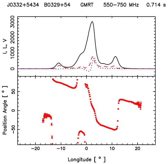
Figure 1.
The above plot shows the average polarization properties of PSR B0329+54 average over the wideband frequency range between 550 and 750 MHz. The top panel shows the total intensity profile shape (black line) and the variation of the linear polarization (red dashed line), along with circular polarization (blue dotted line) across the profile. The bottom panel shows the average PPA traverse that has quite complex features.
The complex nature of the average PPA traverse of PSR B0329+54 was first unraveled by [70], as they overlayed the PPAs of single pulses to find two clear tracks separated by 90° that correspond to the two OPMs as well as other PPAs outside the two tracks. Later studies at multiple frequencies confirmed the detection of the two OPM in this pulsar [71]. The single pulses also show the mode changing behaviour, where the radio emission switches between two stable states with different profile shapes [72,73,74,75], but the PPA behaviour is similar in the two emission modes [76]. Figure 2 shows the single-pulse PPA distribution from the u-GMRT observations, with the two PPA tracks clearly visible [70].
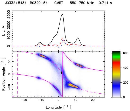
Figure 2.
The top panel shows the average profile of the total intensity (Stokes I; solid black lines), total linear polarization (dashed red line), and circular polarization (Stokes V; dotted blue line) of PSR B0329+54 between 550 and 750 MHz observing frequency. The lower panel shows the single pulse PPA distribution (color scale), along with the RVM fits to the two PPA tracks, shown as dashed and solid magenta lines.
Subsequent single-pulse studies have demonstrated that PPAs of time samples with high levels of linear polarization closely follow the RVM nature [57,77,78]. Figure 3 shows a subset of the PPA behaviour of Figure 2, where the time samples with a linear polarization level in excess 90% have been selected. The two PPA tracks of the OPMs are clearly evident in this plot. Each PPA track can be fit with the RVM using the same values of , , and , and tracks are exactly orthogonal. [71] estimated the absolute direction of the PPA with respect to the fiducial plane, containing the rotation axis and the magnetic dipole, and identified the two tracks as the X-mode (dashed magenta line) in Figure 2 (lower window) and the O-mode (solid magenta line) in Figure 2 (lower window). The radio emission height can be determined from these observations by estimating the aberration-retardation shifts in the PPA, as discussed in the previous section. We found the shift to be , and the corresponding emission height is about 300 km. In Figure 3, it can be seen that in a narrow region around the longitude , which is also close to the SG point, the average linear polarization level goes below 60%. This is due to the large spread of single-pulse PPAs in this longitude range, and we have ignored this narrow region while carrying out the RVM fits. Figure 4 shows a second subset of the PPA behaviour of Figure 2 where the time samples with linear polarization level less than 30% have been selected. The non-orthogonal PPAs are seen in this figure to be present across the profile.
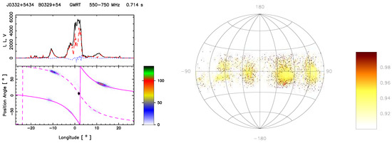
Figure 3.
The above plot shows a subset of the observed polarization behaviour in PSR B0329+54 for time samples with a linear polarization level larger than 90%. In the left window, the top panel shows the average profile with total intensity (Stokes I; solid black lines), total linear polarization (dashed red line), and circular polarization (Stokes V; dotted blue line). The lower panel in the left window shows the single-pulse PPA distribution (color scale) with distinct orthogonal tracks. The RVM fits to the PPAs are also shown as dashed and solid magenta lines in this plot. The right plot shows the Hammer−Aitoff projection of the polarized time samples, with the color scheme representing the fractional polarization level.
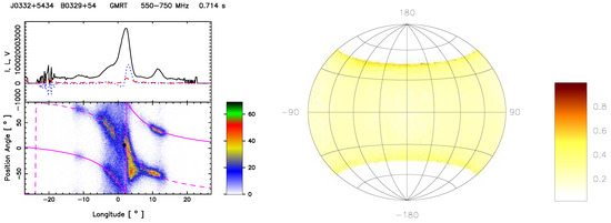
Figure 4.
The above plot shows a subset of the observed polarization behaviour in PSR B0329+54 for time samples with a linear polarization level less than 30%. In the left window, the top panel shows the average profile with total intensity (Stokes I; solid black lines), total linear polarization (dashed red line), and circular polarization (Stokes V; dotted blue line). The lower panel in the left window shows the single-pulse PPA distribution (color scale) with non-orthogonal characteristics. The RVM fits to the PPAs are also shown as dashed and solid magenta lines in this plot. The right window shows the Hammer−Aitoff projection of the polarized time samples, with the color scheme representing the fractional polarization level.
2.3.1. High Levels of Linear Polarization
The presence of individual subpulses with high levels of linear polarization was detected in several earlier studies [79,80], but their origin was unclear. If we consider the situation in Figure 3, where time samples with close to 100% linear polarization levels are shown, the two PPA tracks have identical RVM characteristics with a shift in PPA phase. Although the RVM was proposed for vacuum curvature radiation originating close to the poles of a static magnetic dipole, the two PPA tracks represent plasma effects and can be associated with the natural plasma modes, i.e., t-mode and -mode of the pair plasma (see Discussion in Section 2.2). However, the t-mode and -mode are confined to the plasma, and additional details are required to understand how they transform into the electromagnetic X and O-modes that can escape the plasma and yet retain the vacuum-like PPA characteristics.
The t-mode and -mode have slightly different dispersion relations in the magnetospheric plasma and can propagate independently of each other. It has been noted by [59] that in a slowly varying magnetoionic inhomogeneous plasma, the polarization features in the emission region evolve due to adiabatic walking. At a certain distance, the effect of adiabatic walking is terminated, and the observed polarization behaviour reflects the pattern frozen in at this point. Under these circumstances, it is possible to obtain high levels of linear polarization, but the effect of the emission mechanism on the PPA is lost. On the contrary, the single-pulse observations reported in [77] showed that subpulses with high levels of linear polarization had PPAs across them that closely followed the RVM nature. Also, a recent study [81] shows that by applying the highly polarized time sample criteria, the RVM can be recovered for a large number of pulsars, and for several pulsars, the highly polarized samples follow two parallel RVM-like PPA tracks. These observations hence strongly favour the natural modes in the plasma to be excited by CCR, with the radiation detaching from the magnetosphere almost immediately after they are generated, with little influence of propagation effects like adiabatic walking [82]. Given the fundamental importance of propagation effects on the observed polarization behaviour and their ability to uncover the emission mechanism, we discuss below the possibility in more detail.
Propagation Effect Cannot Explain the High Levels of Linear Polarization
The aberration and retardation effect is likely to affect both the t- and -modes propagating in the plasma, and the effect depends on the emission height from which each mode detaches from the plasma. The t-mode, with vacuum-like dispersion property, remains unaffected by refraction in the medium and propagates along the tangent to the magnetic field line at the point of generation. On the other hand, both branches of the -mode are refracted in the medium and are ducted along the magnetic field lines with different extents. If the t-mode and the -mode detach from the magnetosphere at different heights, the observed PPA tracks should be different. However, the PPA tracks of the two OPMs are observed to be identical, suggesting that the effects of refraction are minimal. As a result, we can conclude that the two modes escape the plasma from the same height.
In order to understand the effect of adiabatic walking on the radio emission, let us assume the presence of a hitherto unknown mechanism that is capable of exciting the normal modes in the relativistic pair plasma. The emission is confined within a narrow cone () centered around the tangent to the local magnetic field. The excitation frequency is close to the plasma frequency and the linear polarization is either parallel or perpendicular to the plane1, but when averaged within the cone, the emission is completely depolarized. The longitude resolution in Figure 3 is 0.16°, and if associated with the angular size of the relativistically emitting cone, the corresponding Lorentz factor is . A mechanism to obtain close to 100% linear polarization from the emission cone, based on the adiabatic walking condition, was proposed by [59]. As the radiation propagates, the curved magnetic field lines bend, and due to adiabatic walking, the emission cone is no longer centered around the tangent to the local field lines, but is directed away from them in their entirety. The polarization vector needs to adjust itself to remain parallel or perpendicular to the plane, and hence in this situation, all the polarization vectors within the cone are pointed in the same direction. Hence, the resultant polarization within the emission cone can reach levels close to 100%. This behaviour is illustrated in Figure 1 of [59] and shows the reorientation of the polarization vector in the emission cone due to adiabatic walking. However, one possible issue in this representation is that the cross-section of the emission cone is assumed to be the same at different heights. On the contrary, the cross-section of the cone keeps on increasing as the emission propagates upwards, as shown in Figure 5 for the t-mode generated at a height of 100 km above the surface. The black lines in the figure correspond to a cone, with , while the green line represents the open magnetic field lines. The radio emission detaches from the plasma at a height of ∼1000 km, where the diverging field lines are still enclosed by the cone. Any averaging effect within this cone would likely result in complete depolarization of the emission [82]. Similar arguments can be made for the -mode as well.

Figure 5.
The above plot shows the schematic of the open dipolar magnetic field lines (in green) above the neutron star surface. The black diverging lines correspond to the rectilinear propagation vector of an emission cone of t-mode generated at a height of 100 km from the surface, where . The radio emission detaches around 1000 km from the surface.
Thus, we conclude that the time samples with high levels of linear polarization seen in Figure 3 cannot be explained by adiabatic walking. Additionally, the symmetrical nature of the PPA traverse requires extreme fine tuning of the plasma parameters. The multiple components in the profile also suggest the presence of non-stationary plasma flow and cannot satisfy the conditions for adiabatic walking, i.e., a slow change in plasma density. It should be noted that in the average profile, the fractional polarization across a wide frequency range can be frequency-dependent, where a higher frequency tends to have more depolarization (see e.g., [48,83,84]). Generally, depolarization is attributed to the mixing of OPMs, and some studies have been devoted to the mechanisms of depolarization ([85,86]) and their frequency dependent behaviour ([87]). In this context, simultaneous wide-band observations of a high linearly polarized time sample in order to explore their frequency dependence can be quite instructive.
High Levels of Linear Polarization from Curvature Radiation
Curvature radiation excites the t and modes, and due to difference in refractive indices, the modes split in the plasma medium and can travel independently as linearly polarized modes, perpendicular and parallel to the curved magnetic field line planes, respectively [88]. There is evidence for the observed PPAs from normal pulsars being either parallel or perpendicular to the curved magnetic field plane. If CCR indeed acts as the radio emission mechanism in pulsars, then several critical conditions related to the coherence and escape of waves need to be satisfied [12]. They suggested that linear electrostatic Langmuir waves could be a possible source of CCR, but this model was not found to be applicable by [89] (see details in Paper II). An alternative theory has been developed where it was suggested that the modulational instability of Langmuir wave can form charge envelopes, or solitons, that are stable enough to emit CCR [15,90].
Ref. [12] also proposed the existence of an inner vacuum gap region above the polar cap where non-stationary plasma flow arises due to intermittent spark discharges and pair plasma cascade, which eventually gives rise to two-stream instability. This model can be used to address a number of observational phenomena, such as subpulse drifting, microstructures in the single pulses, and measurements of the hot polar cap. However, the vacuum gap model does not quite agree with the details of these measurements and requires modification in the form of a partially screened gap, PSG hereafter [91] (see discussion below in Section 4). An illustration of the non-stationary plasma flow from the PSG model is shown in Figure 6. In the dense pair plasma clouds, stable relativistic-charged solitons can be generated at distances of few percent of ; they have a Lorentz factor larger than the Lorentz factor of spark-associated plasma . The solitons while moving along the curved magnetic field lines excite CCR with characteristic frequency, , where is the radius of curvature of the open dipolar field lines. If we use the parameters of PSR B0329+54 and assume typical values of , we get GHz, which lies in the typical radio frequency range. Using the multiplicity factor of the spark-associated plasma, , the characteristic frequency satisfies the condition in PSR B0329+54.
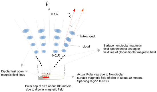
Figure 6.
The above plot shows a schematic of the PSG model (not to scale). Due to non-dipolar magnetic fields on the surface, the actual polar cap (shown as the red region) is smaller than the equivalent dipolar case. The PSG exists above the polar cap where non-stationary spark discharges are triggered, shown as red stars in the figure. The open field line region corresponding to the non-dipolar field lines connects to the global dipolar field (shown as a dashed black line), and the spark discharges form plasma clouds with high-density regions near the center (blue shaded) and low-density regions in between. CCR is generated in the plasma clouds at about , and the radiation enters the inter-cloud region below . The inter-cloud regions are the white spaces enclosed within the open magnetic field line region, where the density of the particles injected from the adjoining sparks become lower, and they are dominated by ions.
The curvature radiation excites the sub-luminal t and modes with polarization directed perpendicularly and parallel to dipolar magnetic field line planes, respectively. In the case of curvature radiation emitted by individual particles under vacuum-like conditions, the power of the perpendicular component is seven times lower than the parallel component. The two modes propagate independently in the plasma medium, with the t-mode having vacuum-like properties and the -mode getting ducted along the magnetic field lines. It has been shown that, despite the power of the t-mode of curvature radiation in plasma being suppressed, the emitted intensity is sufficient to account for the observed pulsar luminosities [88]. In order to estimate the rotation of the polarization plane of the modes, the adiabatic walking condition needs to be evaluated and has the form [59]
Here N is the difference between the refractive index of t and mode, is the change in N as the wave propagates in the medium, k is the wave vector, and is the linear PPA. In the case of curvature radiation from solitons in the radio frequency range, the condition is satisfied and , such that the effects of adiabatic walking are not applicable2 [82,88]. The waves preserve their polarization direction while escaping from the plasma (also see [92]). The mode cannot escape under homogeneous plasma conditions as it gets ducted and eventually undergoes Landau damping. However, is possible if the plasma density has large gradients, and then the wave can successfully escape from the plasma. In the PSG model, the center of the dense clouds has a high pair multiplicity factor (); as one moves towards the boundary between adjacent clouds, the muliplicity factor () decreases to orders of unity. This creates a density gradient in the plasma at the inter-cloud boundary through which the mode can escape [57,82].
A large number of solitons are produced in each plasma cloud, and as the cloud moves along the curved field line, the average emission from the cloud passes into the inter-cloud region. The radiation propagates in a rectilinear manner in the inter-cloud region, and due to the curvature of the field lines, the angle between and the tangent to the dipolar magnetic field, , continues to increase. The plasma clouds are expected to give rise to the individual components seen in the average profile, with typical angular width of about . CCR is generated at heights of where and as the radiation reaches the angle increases to , which is large enough for the radiation to transfer into the inter-cloud region [57]. Beyond this region, does not change with increasing height until , after which the magnetic field lines bend due to sweepback effects. The t and modes from different plasma clouds enter the inter-cloud region and undergo incoherent addition. This process gives rise to the resultant linear polarization and the associated PPA distribution observed in pulsars. The emission process is stochastic, with different clouds having different orientations of the plane, such that averaging will lead to depolarization. From time to time, we expect dominant t or modes from strongly magnetized plasma to emerge from the clouds, and the corresponding X- and O-modes will show up as the clear orthogonal PPA tracks observed in Figure 3. At other times, the emergent emission undergoes incoherent mixing of the t- and -modes in various proportions and orientation, resulting in the low levels of linear polarization and scattered PPAs seen in Figure 4. The plasma clouds can also be associated with the quasi-periodic structures, known as microstructures, observed in single pulses [93,94].
CCR being excited in the plasma clouds and subsequently emerging from the inter-cloud region provides a successful mechanism to explain the highly polarized time samples observed in pulsars, but this model still remains largely qualitative. It has also been suggested that in homogeneous plasma, the cyclotron damping will affect the plasma modes in the upper magnetosphere, preventing the radiation from escaping [95]. However, the inhomogeneities introduced by the PSG model will reduce the damping effect as the waves propagate in the inter-cloud region. Detailed theoretical studies are still necessary to find the escape condition of mode, as well as simulations showing that the incoherent averaging process is able to reproduce the observed polarization characteristics. Our discussions make it clear that propagation effects due to refraction and adiabatic walking have a negligible effect when modifying the radiation features.
2.3.2. Circular Polarization
In early studies of pulsar emission, the circular polarization was expected to be a part of the emission process [96,97,98,99,100,101], although the polarization behaviour is likely to change as the emission propagates within the plasma medium. The circular polarization behaviour of highly polarized time samples from PSR B0329+54 is shown in Figure 3, where the right window represents the Hammer-Aitoff projection of the Poincaré sphere. The spread of the distribution away from the equatorial plane indicates that almost all polarized time samples are elliptically polarized. This suggests that the linearly polarized t- and -modes generated in the inner magnetosphere are partially converted into circularly polarized modes as they propagate further in the outer magnetosphere. The polarization behaviour of PSR B0329+54 corresponding to the time samples with lower levels of linear polarization is shown in Figure 4. The distribution spans a wider azimuthal range on the Poincaré sphere with similar values for both the positive and negative circular polarization. In the entire observing span, shown in Figure 2, the mean level of absolute circular polarization is about 20%, which is typical for normal pulsars [57]. The models of emission mechanism in pulsars need to explain the observed circular polarization that arises due to propagation effects within the plasma at heights between and ∼0.1.
One of the suggested mechanisms for the appearance of circular polarization is the wave-mode coupling that appears due to co-rotation of the magnetosphere [42,59,102,103]. The propagation vector gets tilted with respect to the magnetic field line due to the co-rotation of the magnetosphere and as it travels a distance ; the adiabatic walking condition adjusts the polarization to generate two independent modes parallel and perpendicular to the plane. Eventually, the adiabatic walking is no longer dominant, resulting in the two modes getting coupled to emerge as elliptically polarized waves. The resultant sense of circular polarization is expected to be constant across the profile, but in reality, both, i.e., right and left circular polarization, are observed across the profile. To address this discrepancy, it was suggested that a change in the plasma distribution along the open flux tube can bring about the asymmetric nature in the profiles [102]. But as asserted in the previous section, we have ruled out the possibility of adiabatic walking condition to explain the observed high linear polarization signals. However, the effects of adiabatic walking and wave coupling on the circular polarization need further study using a realistic model of non-stationary plasma flow.
We consider another possibility where the generation of circular polarization requires a breakdown of symmetry in the positive and negative components of the pair plasma. It should be noted that the circular polarization naturally occurs as eigenmodes in an electron-ion plasma. The co-rotational electric field causes the distribution function of electrons and positrons to be slightly different, and the presence of ionic species can further break the gyrotropy. In this case, the normal modes propagating at small angles with respect to the external magnetic field can be circularly polarized [16,103,104]. The absence of gyrotropy has been used to explain the origin of circular polarization using the PSG model [57]. It is convenient to consider a coordinate system [105] along the z-axis, and, introducing , , i.e., , we can obtain the dispersion relation as:
The solution of Equation (3) has the form
Here, depends on the plasma parameters. When then , resulting in circular polarization. In the PSG model, the emission enters the ion-dominated inter-cloud region at a distance . In the inter-cloud region, where and , the radio frequency is higher than the local characteristic frequencies. The wave can propagate rectilinearly, and the angle between the wave vector and the local field, , remains constant for large distances, satisfying the conditions and . It has been shown [57] depends on the pulsar parameters as:
Here is the average Lorentz factor of the electron positron component of the plasma, and where is the radio frequency in Hz. Using parameters for PSR B0329+54 and other typical plasma parameters, radian, , and MHz, we estimate . This suggests that the above mechanism supports the necessary condition for obtaining circular polarization, i.e., , in PSR B0329+54. The observed circular polarization is an incoherent addition from many different clouds, while the sense of circular polarization depends on the viewing geometry.
3. Variation of Spectral Index across the Profile Window
The previous sections have highlighted that the magnetic field has dipolar characteristics at the radio emission heights. The curvature radiation is directly associated with the curvature of field lines. As the LOS traverses across the emission beam, corresponding to the open dipolar field line region, at any given height, the radius of curvature increases from the edge towards the center of the emission beam. The shape of the average profile is determined by the LOS traverse across the emission beam, with distinct physical properties seen in the core component at the center compared to the conal components at the periphery. The CCR from charge bunches predicts a difference in the spectral nature of the flux density between the central core and the peripheral conal components. A proper characterisation of this spectral behaviour provides direct evidence for the emission mechanism in pulsars. Below, we summarize the nature of the average emission beam in the pulsar population and the different efforts in constraining the spectral variation across the emission beam.
3.1. Classification of Profile Morphology and Nature of Emission Beam
The average profile of each pulsar has unique features and characterised by the number of components that can vary between one and five. The components are classified into two major types: the core component that is usually located at the center of the profile and shows a large change in the PPA traverse across it with sign changing circular polarization, and the conal components located around the core with relatively shallow PPA slopes and higher levels of linear polarization [35] (also see discussions above). The pulsar profile also shows significant evolution with frequency. The profile widths become wider at lower frequencies due to the effect of radius-to-frequency mapping, where the lower frequencies originate from higher up the open dipolar field [52]. In addition, the number of components in the profile can also change at different frequencies.
The earliest suggestion about the nature of the emission beam was the “hollow cone” model [106,107] where the emission was expected to originate in a narrow cone surrounding the last open field lines, symmetrically around the magnetic axis. However, the hollow cone model was not adequate to explain all observed profile types and has led to the “Core-Cone” model of the emission beam proposed in a series of works [35,36,37,38,108]. It has the widest applicability in understanding the different profile types. In the core-cone model, the emission beam at any observing frequency comprises of a central core region surrounded by two pairs of nested conal rings forming the inner and outer cones The profile shape is determined by the pulsar geometry and the distance of the LOS traverse from the magnetic axis. When the LOS cuts the emission beam centrally, close to the magnetic axis, they form the core-cone Triple (T) and core-double cone Multiple (M) profile types. Sometimes one side of the conal component in a T profile is weaker, and the profile is classified as . The conal Quadruple Q), conal Triple T), Double (D), and conal Single () profiles represent the cases of the LOS cuts being progressively away from the magnetic axis, missing the central core component, and moving towards the edge of the beam. A core Single () represents a central LOS traverse where the conal components are absent. In many cases, the profiles develop conal outriders at higher frequencies, while the profiles become wider and bifurcates at lower frequencies.
In the initial works, the core-cone model preserved the hollow-cone structure, with the outer cones and inner cones both bordering the outer field line originating at different heights, while the core was expected to arise from the surface. Subsequent works [109,110,111,112] have found that the widths of the core and the conal components have similar distributions with pulsar period and identical lower boundaries. These results confirmed that the core and the conal components originate from similar heights. As a result of the current understanding of the emission beam structure, the core component is associated with the central field lines around the dipolar magnetic axis, the inner cones, and the intermediate field lines between the axis and the open field line boundary, while the outer cones occupy the outermost field lines bordering the boundary. It is expected that the radius of curvature of the magnetic field lines is highest in the core region and progressively decreases towards the inner and outer cones.
Alternative models for the emission beam include the “patchy cone” [113] where the components are expected to arise from similar heights but are distributed randomly within the emission beam. The primary justification for this model comes from the presence of the “partially conal” profiles where the PPAs are asymmetric and the SG point is shifted towards one edge of the profile. Later studies have shown that in most of these cases, the beam shape follows a core-cone structure, with one edge of the profile having a lower intensity most of the time and only appearing during flaring events in the single pulses [56]. In a few other cases, additional components in the form of pre/post-cursor emissions are seen that are not part of the emission beam [114]. There are also suggestions of the emission beam being a “fan beam” with the components arising from emission along flux tubes [100,115,116,117]. The fan beam has been used to explain the bifurcated features seen in the profiles of certain pulsars. However, it is not clear if the characteristics of the different profile morphologies can be explained in this model. Further, the requirement of a tightly packed sparking pattern above the polar cap that gives rise to subpulse drifting (see discussion below) is also difficult to reconcile with a fan beam without conal symmetry.
There are indications that the emission beam shows evolution with the spin-down energy loss () or characteristic age (see e.g., [118]). The profile classes are not distributed uniformly with , with more prevalent in the high range above erg , while the conal profiles corresponding to D and types are usually seen in pulsars with low erg [119,120]. The differences in beam shape presented in [55] are subtle, with the fractional polarization between the two subsets being more prominent. Other possibilities include an increase in the number of sparks in high pulsars with a wider open field line region, which form a large number of closely packed components with blurred boundaries between them [121].
3.2. Measuring Spectral Variation across the Emission Beam
The coherent radio emissions from pulsars have a steep power law spectra between 100 MHz and 10 GHz with spectral index [122,123]. The emission beam studies have shown that the central core component in the profiles is associated with the field lines close to the magnetic axis, where the radius of curvature is larger, while the conal emission occupies the field lines closer to the boundary of the open field line regions, where the magnetic field lines are more curved with relatively smaller values of the radius of curvature. There have been indications that the core components have steeper spectra compared to the cones, e.g., the appearance of conal outriders at higher frequencies in profile types. However, detailed measurements of the relative spectral indices of the components have not been carried out due to several challenges in estimating the flux density levels of the profile. This primarily arises from the lack of proper instrumental calibration required to scale the measured signal to the appropriate flux densities. In addition, the pulsar signal is also affected by scintillation over timescales varying between several minutes (diffractive scintillation) and extending to several months (refractive scintillation) [124]. As a result, the proper estimation of the flux densities requires averaging over long timescales, which is only available for relatively few pulsars at specific frequencies [125,126,127,128,129]. Other issues affecting flux density estimates, particularly at lower frequencies, involve interstellar scattering [130]. One attempt to measure the spectral index of the different components in the profile by [108] used the Gaussian fitting technique to identify the components. No clear trend of spectral variation between components of the profile was found in this work. However, the Gaussian components were often displaced from actual profile components and made it difficult to have a direct connection between them.
A way around the issue of the non-availability of proper flux calibration of the profiles as well as variations due to interstellar scintillation has been devised in our previous works [131], where it was noticed that these effects introduce an unknown but identical multiplicative scaling for all components in the profile. As a result, the ratio between the component intensities is expected to be invariant of the measurement conditions and can be used to estimate the relative spectral index of the core with the inner and outer conal components as follows:
The estimations of the relative spectral index () of the core and the conal components are possible in pulsar profiles with central LOS traverses, such that both the core and conal components are present, i.e., T, , and M type profiles. In addition, the relative spectral index between the inner and outer conal pairs () can be carried out in M, , and profiles.
Figure 7 shows the frequency evolution of the profile shape of PSR B1821+05 that has a T-type profile. The figure shows the measured profiles at six frequency bands between 100 MHz and 5 GHz. At the lowest frequency of 135 MHz only the core component is seen, while the conal components are too weak to be detected. With increasing frequency, the relative intensity of the conal components increases with respect to the core, and the cones dominate the profile at frequencies above 1 GHz. Figure 8 shows the spectral plot of the relative intensities between the core and the cone () between 100 MHz and 10 GHz, with the estimated spectral index (see line in Figure 8), demonstrating the core to have a much steeper spectral index compared to the conal emission. At the lowest frequency range, the conal components are not visible in the profile and hence the relative intensities cannot be measured. The core emission at 4.8 GHz merges with the trailing conal component (see Figure 7, bottom right panel), leading to imprecise measurements. As a result, at the highest frequency, the relative intensities deviate from the linear spectral behaviour.
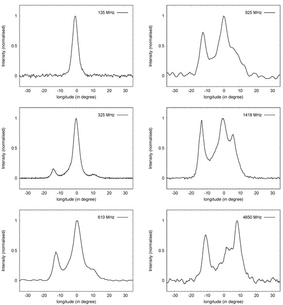
Figure 7.
The Figure shows the T-type average profile of PSR B1821+05 at 6 different frequencies at 135 MHz (top left), 325 MHz (middle left), 610 MHz (bottom left), 925 MHz (top right), 1408 MHz (middle right), and 4850 MHz (bottom right). The core component in the center of the profile is stronger at the lower frequencies and becomes weaker compared to the surrounding cones with increasing frequency.
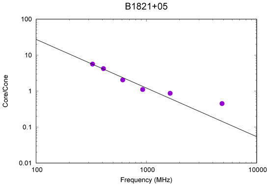
Figure 8.
The figure shows the frequency evolution of the relative intensities of the core and the conal components () of PSR B1821+05 between 100 MHz and 10 GHz. The power law fit to the relative spectral index shown by a solid black line has a spectral index of −1.55 ± 0.1.
Similar studies have been carried out in around 50 pulsars having both core and conal components in their profiles [131], and in all cases, the core component has a steeper spectra than the cones, with varying between −0.4 and −2.0. The radius of curvature of the magnetic field lines are expected to change between the core and the conal components, and the only known emission mechanism that has direct dependence on the radius of curvature of the field lines is CCR from charge bunches. As a result, the observational result of the core having a steeper spectral index than the conal components within the pulsar profile strongly favours the radio emission mechanism in pulsars to be CCR.
4. Subpulse Drifting: Window into Inner Acceleration Region
The CCR from charge bunches needs the presence of a multi-component electron-positron plasma in the form of plasma clouds, separated by less dense regions filled with positively charged ions, and requires a non-stationary plasma flow. In this section, we briefly summarize our understanding of the plasma generation process in pulsars and its observational signature in the form of subpulse drifting.
The plasma is expected to be generated in an inner acceleration region (IAR) above the polar cap, extending to heights of around 10–100 m. In one of the earlier studies by [12], the IAR was considered to be a vacuum gap (IVG). The IVG is characterised by very high magnetic fields ( G) as well as large electric potential difference ( V) along the magnetic field. Under these extreme conditions, regular breakdown of the gap in the form of spark discharges is expected. This mechanism of plasma generation is possible in pulsars where (here is the angular velocity of the neutron star), such that positively charged particles are accelerated away from the stellar surface while the negatively charged particles are accelerated towards the surface. In the IVG, the electron-positron pairs are produced from ambient -ray photons and accelerated to high energies with the Lorentz factor [10]. The positrons are accelerated away from the gap and produce additional -ray photons due to curvature radiation or inverse compton scattering as they propagate along the curved magnetic field lines. These additional -ray photons generate further pairs, resulting in a cascading effect. Effective breakdown of the gap requires the magnetic field to be highly curved and non-dipolar in such a nature that high-energy -ray photons can be produced. In this process, a primary plasma beam comprising high energetic positrons is formed.
When the charge density in the IVG equals the Golreich-Julian density, [9], the electric potential difference along the magnetic field is fully screened, and pair production is halted. The potential difference reappears once the plasma escapes the gap due to inertial motion and the next sparking event is triggered, forming the non-stationary plasma flow. The primary particles continue to produce additional pairs outside the IAR to form clouds of secondary-pair plasma that are considerably less energetic, with Lorentz factors () between 100 and 1000, and have high multiplicity, [10]. The CCR develops in these spark-associated secondary plasma clouds that stream outwards along the open magnetic field line region.
Subsequent works have revealed several limitations of the IVG model of IAR. The back-flowing electrons produced during sparking are expected to heat the surface to temperatures of K, which is near the critical level for ions () to be emitted freely from the surface and screen the potential difference along the magnetic field [132,133]. In a purely vacuum gap, there is no mechanism to constrain the lateral size of the sparks, as there is unscreened potential difference in the boundary between two adjacent sparks. As a result, the primary particles cannot be confined to any specific location within the IVG but likely scatter in the direction opposite to the principal normal to the curvature of the local magnetic field lines [132].
In order to address the heating of the surface due to back-flowing electrons during sparking, an updated model of the IAR has been proposed. It has been suggested that the IAR is not a complete vacuum but has a steady supply of positively charged ions from the surface and forms a partially screened gap (PSG) [91]. The potential difference along the gap is reduced by a screening factor , where is the average density of ions in the gap. In a PSG, the sparking process is primarily a mechanism to regulate the surface temperature around of ionic free flow. When the surface temperature () is close to , there is a free flow of ions from the surface and the potential difference along the IAR is screened. As the surface cools down and , the supply of ions from the surface decreases such that the density goes below and the potential difference appears in the IAR. This starts the sparking process, and the primary plasma is produced along with the back-flowing electrons that once again heat the surface to a critical level, thereby terminating the spark. The typical timescale for each spark to develop and empty the IAR is around 30 µs, while the surface cools rapidly once the sparking stops with a typical cooling time of 30 ns.
When a spark starts at a location within IAR, it also spreads out across the field lines until enough particles are produced to heat the surface and screen the potential difference along the magnetic field. As a result, the lateral size of the sparks () is regulated by the energy that needs to be deposited on the surface for the thermal regulation process. The PSG is the only known mechanism for confining sparks in the IAR, where the sparking location is determined by the surface temperature profile. The sparks are formed in a tightly packed manner for effective thermal regulation of the surface. The peak density is near the center of the spark, and the density gradually decreases towards the edge, with the boundary between two sparks dominated by the ions emitted from the surface. The primary plasma produced in the sparks leaves the IAR, and it gives rise to the columns of secondary plasma clouds. The inter-cloud regions correspond to the boundary between sparks and are dominated by the positively charged ions. For a typical normal pulsar, the Lorentz factor of the secondary pair plasma is and the Lorentz factor of the ion component , where superscripts “sp” and “isp” stand for the spark and interspark region. The multiplicity at the center of the spark, which gradually becomes in the interspark region. The Lorentz factor of the ion in the interspark region is . In terms of pulsar parameters P and and , the plasma frequency of the pair plasma is and the ion plasma frequency is , where ion species is used (see [57] for these estimates).
When the pulsar magnetosphere is filled up with , the plasma corotates with the star due to drift. During sparking, the plasma density in the IAR is less than and plasma no longer corotates with the star. The sparks during their lifetimes lag behind the rotation of the star [134], and the location of maximum heating/cooling shifts opposite to the direction of the rotation as the spark develops. Once the plasma empties and the surface cools down, the next spark is formed slightly shifted in the direction opposite to the rotation. This lack of corotation is imprinted in the plasma clouds as they move along the open field line region and emit radio waves. The effect is seen in the single-pulse behaviour of certain pulsars as the phenomenon of subpulse drifting [135,136,137]. Subpulse drifting is intricately connected to the conditions in the IAR, like the potential difference along the magnetic field, the nature of non-dipolar magnetic fields, the surface conditions, etc. We describe below the measurement of the drifting behaviour in pulsars and how these results can be used to obtain observational evidence for the presence of non-dipolar fields above the stellar surface and for the IAR to be a PSG. This in turn puts the presence of plasma clouds in the open field line region, the presence of multi-component plasma, and the dominance of ions between plasma clouds, on a firm observational footing.
4.1. Drift Phase Variations: Evidence of Non-Dipolar Magnetic Field
The single-pulse emission in pulsars consists of one or more constituents that are called subpulses. In certain cases, the subpulses show systematic periodic shifts, and the phenomenon is called subpulse drifting, which was first discovered by [138]. The drifting behaviour is best visualized when the single pulses are represented in the form of a pulse stack, which is a two-dimensional plot with the rotation longitude along the x-axis and the pulse number in the y-axis. Two examples of subpulse drifting are shown in Figure 9. The nature of the drifting behaviour is associated with the profile morphology and LOS geometry [119]. The pulsars with large shifts of the subpulses across the emission window have conal profiles of and D types (see previous section). On the contrary, the M-type profile usually has very little shift in the position of the subpulses but periodic modulation of intensity in their conal components. The central core component in these profiles does not show any drift behaviour. The intermediate LOS profiles like and show complex drift behaviour with reversals in drift direction, also known as bi-drifting, between different components of the profile in a few cases. The drifting behaviour is measured using the Fourier transformation technique, like the longitude resolve fluctuation spectra (LRFS) [139], where Fourier transforms are carried out along each longitude range of the pulse stack for a fixed number of pulses. The drifting periodicity (), which represents the time interval between subpulses repeating at any longitude, is seen as a peak frequency in the LRFS. The phase variations corresponding to the peak frequency show the track of the subpulses across the profile window (see Figure 10).
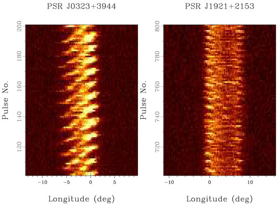
Figure 9.
The figure shows the single-pulse stack of PSR J0323+3944 (or PSR B0320+39) at 333 MHz (left panel) and PSR J1921+2153 (or PSR B1919+21) at 610 MHz (right panel), where the subpulse drifting phenomenon is clearly observed. The data were obtained from the GMRT; for details, see [119].
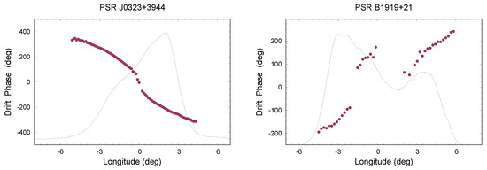
Figure 10.
The figure shows the phase variation of the drifting subpulses across the profile of PSR J0323+3944 at 333 MHz (left panel) and PSR B1919+21 at 610 MHz (right panel). The black dotted line correspond to the average profile and the red points show the subpulse drifting phase variation across the profile.
As discussed earlier, the sparks in a PSG are formed in tightly packed configuration and lag behind the rotation motion of the star [134]. The subsequent sparks are formed slightly shifted in the direction opposite to the rotation of the star. In addition, the well-defined polar cap boundary separating the open and closed field line region of the magnetosphere constrains the later sparks to be formed along the boundary. Hence, the two-dimensional sparking pattern in the IAR evolves with time along two different directions, in a clockwise and counterclockwise manner in the two halves of the polar cap. In the center of the IAR, the sparks are formed at regular intervals in roughly the same location since there is no space for shifting. The central sparks make up the core component in the profile that does not show any drifting behaviour.
The drifting periodicity as well as the phase variations can be associated with the sparking process in the IAR. The drifting periodicity measures the electric potential difference and particularly the screening factor, , of PSG and will be discussed in the next subsection. The phase variations across the profile trace the evolutionary track of the sparking pattern along the projection of the LOS (see Figure 11, left panel). As a result, the phase behaviour has information regarding the shape of the polar cap, which is determined by the nature of the surface magnetic field. In the case of a purely dipolar field, the phase variations are expected to be mostly linear with small deviations near the edge of the inner and outer cones. The expected phase variations in drifting for an intermediate LOS cut located midway between the magnetic axis and the polar cap edge have been simulated and shown in Figure 11 (see [134] for details). The phase behaviour is mostly linear across the entire profile, with small deviations at the crossing between the inner and the outer cones, and near the edges. The measured phase variations for two pulsars PSR J0323+3944 (left panel) and PSR B1919+21 (right panel) are shown in Figure 10. The phases show a larger deviation from linearity and significant jumps between components, confirming that the surface magnetic fields in pulsars are non-dipolar in nature. The direction of the slope of the phase changes is reversed in these two pulsars and has a degenerate origin, either due to the drifting periodicity being aliased or the local magnetic field on the surface being highly twisted [134].
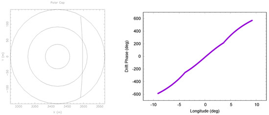
Figure 11.
The figure shows the modelled phase variations of subpulse drifting from a polar cap with a dipolar magnetic field. (The left panel) shows the LOS traverse across the polar cap, where the three concentric rings demarcate the core, inner, and outer conal regions. The LOS traverse cuts across the polar cap about halfway between the axis and the open field line boundary. (The right panel) shows the simulated phase variations of the drifting subpulses for this configuration.
4.2. Dependence of Drift Periodicity with : Evidence of Partially Screened Gap
The drifting periodicity is the time taken by subsequent sparks to lag behind the extent of the spark diameter, such that the subpulse peaks appear at the same longitude in the emission window. The speed at which the sparking pattern shifts in the gap is , and the repetition time is estimated as [134]; here is the angle of the local magnetic field with the rotation axis.
The total energy outflow from the PSG () due to the outflowing plasma can be estimated as [137]:
Here, , and is the area of the polar cap. The quantity is invariant of the nature of the surface fields due to conservation of magnetic flux and can be estimated as
Additionally, is also obtained from P and in the form erg . The ratio between and has the form:
Here, erg . The PSG model provides a direct connection between two independent measurable pulsars, and , which have the form
i.e., we obtain a dependence between the two quantities.
The distribution of with has been estimated in a number of works [119,137,140] and reproduced in Figure 12, with additional measurements from recent works added to the figure [141,142,143,144,145,146,147,148]. The drifting behaviour is often conflated with the periodic nulling and periodic modulation features seen in pulsars [149], that have quasi-periodic variation unrelated to the sparking process in the IAR [140]. We have restricted the in Figure 12 to cases with clear indications of drifting in the single pulses. Although there is a prospect of aliasing associated with the measurements, where any intrinsic is seen as a higher periodic feature , the general trend of the anti-correlation between and is evident in Figure 12. Additional support for the presence of such dependence is also seen in the grouping of periodicities at the alias boundary near erg . Some pulsars above this range show an increase in their , suggesting an aliased measurement, which will be expected from anti-correlation. The figure also shows the dependence (black line) of the PSG model, which is consistent with the distribution. The scatter in the plot is also explained in this model due to the dependence on parameters like and , which are likely to vary between different pulsars. The presence of anti-correlation between two independent measurables, and , provide strong observational justification for the IAR to be a PSG.
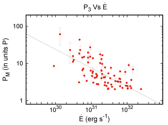
Figure 12.
The figure shows the distribution of drifting periodicity () with the spin-down energy loss (). The black line shows the expected dependence from the partially screened gap model of the inner acceleration region.
5. Summary
The identification of highly linearly polarized signals following the RVM in conjunction with the findings that pulsar radio emissions from normal pulsars detach from regions below 0.1 strongly suggests that CCR is the radio emission mechanism in pulsars. The OPMs indicate that the linearly polarized orthogonal modes are excited in strongly magnetized pair plasma that can reach the observer as X- and O-mode. The observed circular polarization suggests the presence of an ion component in the plasma. The multiple-component average profiles, the single-pulse quasi-periodic structure, and subpulse drifting require non-stationary plasma flow and strong non-dipolar surface magnetic fields. Hence, this observational evidence provides the framework for the necessary conditions for CCR to develop.
CCR from charge bunches has been considered as a plausible candidate for radio emission mechanism from the beginning of pulsar research. However, there are still some questions raised regarding a suitable theory that can justify the existence of stable charge bunches in pulsar plasma. Alternate emission mechanisms, such as the maser mechanism, have also been suggested for the radio emission in pulsars; however, these theories do not have adequate observational support. Studies addressing the issue of charge bunch formation, on the other hand, resulted in identifying the existence of stable relativistic charged solitons in the pulsar plasma [15,90,150]. These studies are performed using the one-dimensional approximation, whereas realistically, stable charge bunch formation needs to be established in two or three dimensions. The overwhelming observational evidence for CCR in pulsars strongly motivates theoretical research in these directions. In the accompanying article by Melikidze, Mitra & Basu the development and current state of the theory of charge bunch formation in pulsar plasma is reviewed.
The enhanced sensitivity of radio telescopes in conjunction with improved data analysis methods in recent years have revealed a plethora of interesting new phenomena from pulsars. While we are fairly confident that the radio emission mechanism from normal pulsars is CCR, there are other issues that still remain unclear. Below we list some of these key problems associated with the pulsar activity.
- The origin and shape of the pulsar emission beam and its evolution with (see e.g., [118]).
- The physical origin of the evolution of average profile width, component width and component separation with frequency, and their dependence on the emission height (see accompanying paper Melikidze, Mitra & Basu, also see e.g., [52]).
- The origin of inter-pulse emission and the post/pre-cursor and off-pulse emission outside the main pulse window (e.g., [114,151,152,153]).
- The complete absence of subpulse drifting in pulsars with erg and also in around 50% of the population below this limit (e.g., [119,136,149]).
- What causes the phenomenon of mode (or state) changing and to explain the observed correlation/anticorrelation between radio and X-ray intensities during mode changing [154]. Also what causes the weak emission detected in the null state of pulsars [155,156].
- How does pulsar signals escape the pulsar magnetosphere? (see e.g., [82,92])
- It is worth mentioning that, unlike normal pulsars, in millisecond pulsars the location of the radio emission region has not been constrained and as a result the coherent radio emission mechanism is still unknown (see e.g., [157,158,159]) ?
- What is the origin of radio emission from Magnetars (see e.g., [160])?
The above list is not exhaustive but gives a flavour of the exciting scientific problems that can be explored in the future.
Author Contributions
All authors have contributed equally to this paper. All authors have read and agreed to the published version of the manuscript.
Funding
D.M. acknowledges the support of the Department of Atomic Energy, Government of India, under project No. 12-R&DTFR-5.02-0700. This work was supported by the grant 2020/37/B/ST9/02215 of the National Science Centre, Poland.
Acknowledgments
We thank the staff of the GMRT, who made these observations possible.
Conflicts of Interest
The authors declare no conflict of interest.
Abbreviations
The following abbreviations are used in this manuscript:
| CCR | Coherent Curvature Radiation |
| GMRT | Giant Metrewave Radio Telescope |
| IAR | Inner Acceleration Region |
| IVG | Inner Vacuum Gap |
| LOS | Line Of Sight |
| LRFS | Longitude Resolve Fluctuation Spectra |
| -mode | Longitudinal Transverse mode |
| OPM | Orthogonal Polarization Mode |
| O-mode | Ordinary mode |
| PPA | Polarization Position Angle |
| PSG | Partially Screened Gap |
| RVM | Rotating Vector Model |
| SG | Steepest Gradient |
| t-mode | Transverse mode |
| u-GMRT | upgraded Giant Metrewave Radio Telescope |
| X-mode | Extraordinary mode |
Notes
| 1 | For example the linear acceleration mechanism excites the O-mode and has polarization oriented parallel to the k − B plane |
| 2 | Note that [59] found adiabatic walking to be important as they were considering an emission mechanism where the radio frequency is close to the characteristic frequency, i.e., , and has large values. |
References
- Hewish, A.; Bell, S.J.; Pilkington, J.D.H.; Scott, P.F.; Collins, R.A. Observation of a Rapidly Pulsating Radio Source. Nature 1968, 217, 709–713. [Google Scholar] [CrossRef]
- Gold, T. Rotating Neutron Stars and the Nature of Pulsars. Nature 1969, 221, 25–27. [Google Scholar] [CrossRef]
- Large, M.I.; Vaughan, A.E.; Wielebinski, R. Pulsar Search at the Molonglo Radio Observatory. Nature 1968, 220, 753–756. [Google Scholar] [CrossRef]
- Staelin, D.H.; Reifenstein, E.C., III. Pulsating Radio Sources near the Crab Nebula. Science 1968, 162, 1481–1483. [Google Scholar] [CrossRef] [PubMed]
- Comella, J.M.; Craft, H.D.; Lovelace, R.V.E.; Sutton, J.M. Crab Nebula Pulsar NP 0532. Nature 1969, 221, 453–454. [Google Scholar] [CrossRef]
- Cocke, W.J.; Disney, M.J.; Taylor, D.J. Discovery of Optical Signals from Pulsar NP 0532. Nature 1969, 221, 525–527. [Google Scholar] [CrossRef]
- Lynds, R.; Maran, S.P.; Trumbo, D.E. Optical Identification and Observations of the Pulsar NP 0532. Astrophys. J. Lett. 1969, 155, L121. [Google Scholar] [CrossRef]
- Ginzburg, V.L.; Zheleznyakov, V.V.; Zaitsev, V.V. Coherent Mechanisms of Radio Emission and Magnetic Models of Pulsars. Astrophys. Space Sci. 1969, 4, 464–504. [Google Scholar] [CrossRef]
- Goldreich, P.; Julian, W.H. Pulsar Electrodynamics. Astrophys. J. 1969, 157, 869. [Google Scholar] [CrossRef]
- Sturrock, P.A. A Model of Pulsars. Astrophys. J. 1971, 164, 529. [Google Scholar] [CrossRef]
- Ginzburg, V.L.; Zhelezniakov, V.V. On the pulsar emission mechanisms. Annu. Rev. Astron Astrophys. 1975, 13, 511–535. [Google Scholar] [CrossRef]
- Ruderman, M.A.; Sutherland, P.G. Theory of pulsars: Polar gaps, sparks, and coherent microwave radiation. Astrophys. J. 1975, 196, 51–72. [Google Scholar] [CrossRef]
- Qiao, G. A mechanism for core emission of pulsars. Vistas Astron. 1988, 31, 393–397. [Google Scholar] [CrossRef]
- Qiao, G.J. Inverse Compton scattering (ICS) plays an important role in pulsar emission. In High Energy Astrophysics: Supernovae, Remnants, Active Galaxies, Cosmology; Springer: Berlin/Heidelberg, Germany, 1988; p. 88. [Google Scholar]
- Melikidze, G.I.; Gil, J.A.; Pataraya, A.D. The Spark-associated Soliton Model for Pulsar Radio Emission. Astrophys. J. 2000, 544, 1081–1096. [Google Scholar] [CrossRef]
- Kazbegi, A.Z.; Machabeli, G.Z.; Melikidze, G.I. On the circular polarization in pulsar emission. Mon. Not. RAS 1991, 253, 377. [Google Scholar] [CrossRef]
- Melrose, D.B. Coherent Radio Emission from Pulsars. Philos. Trans. R. Soc. Lond. Ser. A 1992, 341, 105–115. [Google Scholar] [CrossRef]
- Melrose, D.B. The models for radio emission from pulsars—The outstanding issues. J. Astrophys. Astron. 1995, 16, 137–164. [Google Scholar] [CrossRef]
- Melrose, D.B.; Rafat, M.Z.; Mastrano, A. Pulsar radio emission mechanisms: A critique. Mon. Not. RAS 2021, 500, 4530–4548. [Google Scholar] [CrossRef]
- Hardee, P.E.; Rose, W.K. Wave production in an ultrarelativistic electron-positron plasma. Astrophys. J. 1978, 219, 274–287. [Google Scholar] [CrossRef]
- Arons, J.; Barnard, J.J. Wave Propagation in Pulsar Magnetospheres: Dispersion Relations and Normal Modes of Plasmas in Superstrong Magnetic Fields. Astrophys. J. 1986, 302, 120. [Google Scholar] [CrossRef]
- Shapakidze, D.; Machabeli, G.; Melikidze, G.; Khechinashvili, D. Quasilinear theory of Cherenkov-drift instability. Phys. Rev. E 2003, 67, 026407. [Google Scholar] [CrossRef] [PubMed]
- Radhakrishnan, V.; Cooke, D.J. Magnetic Poles and the Polarization Structure of Pulsar Radiation. Astrophys. Lett. 1969, 3, 225. [Google Scholar]
- Wampler, E.J.; Scargle, J.D.; Miller, J.S. Optical Observations of the Crab Nebula Pulsar. Astrophys. J. Lett. 1969, 157, L1. [Google Scholar] [CrossRef]
- Böhm-Vitense, E. The Pulsar NP 0532 and the Implications of the Oblique-Rotator Hypothesis. Astrophys. J. Lett. 1969, 156, L131. [Google Scholar] [CrossRef]
- Morris, D.; Berge, G.L. Measurements of the polarization and angular extent of the decimetric radiation of Jupiter. Astrophys. J. 1962, 136, 276–282. [Google Scholar] [CrossRef]
- du Plessis, L.; Wadiasingh, Z.; Venter, C.; Harding, A.K. Constraining the Emission Geometry and Mass of the White Dwarf Pulsar AR Sco Using the Rotating Vector Model. Astrophys. J. 2019, 887, 44. [Google Scholar] [CrossRef]
- Radhakrishnan, V. Fifteen Months of Pulsar Astronomy. Publ. Astron. Soc. Aust. 1969, 1, 254–263. [Google Scholar] [CrossRef]
- Lerche, I. On the Motion of Current Sheets, and the Radio, Optical, and X-ray Emission from Pulsars. II. Pulse Structure, Polarization, Time-Varying Features, and Tight-Beam Emission. Astrophys. J. 1970, 160, 1003. [Google Scholar] [CrossRef]
- Manchester, R.N.; Taylor, J.H.; Huguenin, G.R. Observations of pulsar radio emission. II. Polarization of individual pulses. Astrophys. J. 1975, 196, 83–102. [Google Scholar] [CrossRef]
- Manchester, R.N. Orthogonal Polarization in Pulsar Radio Emission. Publ. Astron. Soc. Aust. 1975, 2, 334–336. [Google Scholar] [CrossRef]
- Backer, D.C.; Rankin, J.M.; Campbell, D.B. Orthogonal mode emission in geometric models of pulsar polarisation. Nature 1976, 263, 202–207. [Google Scholar] [CrossRef]
- Cocke, W.J.; Pacholczyk, A.G. Theory of the polarization of pulsar radio radiation. Astrophys. J. Lett. 1976, 204, L13–L15. [Google Scholar] [CrossRef]
- Melrose, D.B.; Stoneham, R.J. The natural wave modes in a pulsar magnetosphere. Publ. Astron. Soc. Aust. 1977, 3, 120–122. [Google Scholar] [CrossRef]
- Rankin, J.M. Toward an empirical theory of pulsar emission. I. Morphological taxonomy. Astrophys. J. 1983, 274, 333–358. [Google Scholar] [CrossRef]
- Rankin, J.M. Toward an Empirical Theory of Pulsar Emission. IV. Geometry of the Core Emission Region. Astrophys. J. 1990, 352, 247. [Google Scholar] [CrossRef]
- Rankin, J.M. Toward an Empirical Theory of Pulsar Emission. VI. The Geometry of the Conal Emission Region. Astrophys. J. 1993, 405, 285. [Google Scholar] [CrossRef]
- Rankin, J.M. Toward an Empirical Theory of Pulsar Emission. VI. The Geometry of the Conal Emission Region: Appendix and Tables. Astrophys. J. Suppl. 1993, 85, 145. [Google Scholar] [CrossRef]
- Ferguson, D.C. The Optical Polarization of the Crab Nebula Pulsar. I. a Relativistic Vector Model. Astrophys. J. 1973, 183, 977–986. [Google Scholar] [CrossRef]
- Ferguson, D.C. The generalized single-vector polarization model for pulsars. I. Theory. Astrophys. J. 1976, 205, 247–260. [Google Scholar] [CrossRef]
- Shitov, Y.P. Pulsar Radio Polarization and the Magnetic Field Twist Effect. Sov. Astron. 1985, 29, 33–39. [Google Scholar]
- Barnard, J.J. Probing the Magnetic Field of Radio Pulsars: A Reexamination of Polarization Position Angle Swings. Astrophys. J. 1986, 303, 280. [Google Scholar] [CrossRef]
- Blaskiewicz, M.; Cordes, J.M.; Wasserman, I. A Relativistic Model of Pulsar Polarization. Astrophys. J. 1991, 370, 643. [Google Scholar] [CrossRef]
- Hibschman, J.A.; Arons, J. Polarization Sweeps in Rotation-powered Pulsars. Astrophys. J. 2001, 546, 382–393. [Google Scholar] [CrossRef]
- Gangadhara, R.T. Pulsar Radio Emission Altitude from Curvature Radiation. Astrophys. J. 2004, 609, 335–339. [Google Scholar] [CrossRef]
- Yuen, R.; Melrose, D.B. Visibility of Pulsar Emission: Motion of the Visible Point. Publ. Astron. Soc. Aust. 2014, 31, e039. [Google Scholar] [CrossRef]
- Phillips, J.A. Radio Emission Altitudes in the Pulsar Magnetosphere. Astrophys. J. 1992, 385, 282. [Google Scholar] [CrossRef]
- Xilouris, K.M.; Kramer, M.; Jessner, A.; Wielebinski, R.; Timofeev, M. Emission properties of pulsars at mm-wavelengths. Astron. Astrophys. 1996, 309, 481–492. [Google Scholar]
- Kijak, J.; Gil, J. Radio emission altitudes in pulsar magnetospheres. Mon. Not. RAS 1997, 288, 631–637. [Google Scholar] [CrossRef]
- von Hoensbroech, A.; Xilouris, K.M. Does radius-to-frequency mapping persist close to the pulsar surface? Astron. Astrophys. 1997, 324, 981–987. [Google Scholar]
- Kijak, J.; Gil, J. Radio emission regions in pulsars. Mon. Not. RAS 1998, 299, 855–861. [Google Scholar] [CrossRef]
- Mitra, D.; Rankin, J.M. Toward an Empirical Theory of Pulsar Emission. VII. On the Spectral Behavior of Conal Beam Radii and Emission Heights. Astrophys. J. 2002, 577, 322–336. [Google Scholar] [CrossRef]
- Kijak, J.; Gil, J. Radio emission altitude in pulsars. Astron. Astrophys. 2003, 397, 969–972. [Google Scholar] [CrossRef]
- Mitra, D.; Li, X.H. Comparing geometrical and delay radio emission heights in pulsars. Astron. Astrophys. 2004, 421, 215–228. [Google Scholar] [CrossRef]
- Weltevrede, P.; Johnston, S. Profile and polarization characteristics of energetic pulsars. Mon. Not. RAS 2008, 391, 1210–1226. [Google Scholar] [CrossRef]
- Mitra, D.; Rankin, J.M. Toward an Empirical Theory of Pulsar Emission. IX. On the Peculiar Properties and Geometric Regularity of Lyne and Manchester’s “PArtial Cone” Pulsars. Astrophys. J. 2011, 727, 92. [Google Scholar] [CrossRef]
- Mitra, D.; Melikidze, G.I.; Basu, R. Meterwavelength Single Pulse Polarimetric Emission Survey. VI. Toward Understanding the Phenomenon of Pulsar Polarization in Partially Screened Vacuum Gap Model. Astrophys. J. 2023, 952, 151. [Google Scholar] [CrossRef]
- Posselt, B.; Karastergiou, A.; Johnston, S.; Parthasarathy, A.; Oswald, L.S.; Main, R.A.; Basu, A.; Keith, M.J.; Song, X.; Weltevrede, P.; et al. The Thousand Pulsar Array program on MeerKAT—IX. The time-averaged properties of the observed pulsar population. Mon. Not. RAS 2023, 520, 4582–4600. [Google Scholar] [CrossRef]
- Cheng, A.F.; Ruderman, M.A. A theory of subpulse polarization patterns from radio pulsars. Astrophys. J. 1979, 229, 348–360. [Google Scholar] [CrossRef]
- Helfand, D.J.; Gotthelf, E.V.; Halpern, J.P. Vela Pulsar and Its Synchrotron Nebula. Astrophys. J. 2001, 556, 380–391. [Google Scholar] [CrossRef]
- Lai, D.; Chernoff, D.F.; Cordes, J.M. Pulsar Jets: Implications for Neutron Star Kicks and Initial Spins. Astrophys. J. 2001, 549, 1111–1118. [Google Scholar] [CrossRef]
- Johnston, S.; Hobbs, G.; Vigeland, S.; Kramer, M.; Weisberg, J.M.; Lyne, A.G. Evidence for alignment of the rotation and velocity vectors in pulsars. Mon. Not. RAS 2005, 364, 1397–1412. [Google Scholar] [CrossRef]
- Rankin, J.M. Further Evidence for Alignment of the Rotation and Velocity Vectors in Pulsars. Astrophys. J. 2007, 664, 443–447. [Google Scholar] [CrossRef]
- Noutsos, A.; Kramer, M.; Carr, P.; Johnston, S. Pulsar spin-velocity alignment: Further results and discussion. Mon. Not. RAS 2012, 423, 2736–2752. [Google Scholar] [CrossRef]
- Noutsos, A.; Schnitzeler, D.H.F.M.; Keane, E.F.; Kramer, M.; Johnston, S. Pulsar spin-velocity alignment: Kinematic ages, birth periods and braking indices. Mon. Not. RAS 2013, 430, 2281–2301. [Google Scholar] [CrossRef]
- Force, M.M.; Demorest, P.; Rankin, J.M. Absolute polarization determinations of 33 pulsars using the Green Bank Telescope. Mon. Not. RAS 2015, 453, 4485–4499. [Google Scholar] [CrossRef]
- Swarup, G.; Ananthakrishnan, S.; Kapahi, V.K.; Rao, A.P.; Subrahmanya, C.R.; Kulkarni, V.K. The Giant Metre-Wave Radio Telescope. Curr. Sci. 1991, 60, 95. [Google Scholar]
- Gupta, Y.; Ajithkumar, B.; Kale, H.S.; Nayak, S.; Sabhapathy, S.; Sureshkumar, S.; Swami, R.V.; Chengalur, J.N.; Ghosh, S.K.; Ishwara-Chandra, C.H.; et al. The upgraded GMRT: Opening new windows on the radio Universe. Curr. Sci. 2017, 113, 707–714. [Google Scholar] [CrossRef]
- Johnston, S.; Kramer, M.; Karastergiou, A.; Keith, M.J.; Oswald, L.S.; Parthasarathy, A.; Weltevrede, P. The Thousand-Pulsar-Array programme on MeerKAT—XI. Application of the rotating vector model. Mon. Not. RAS 2023, 520, 4801–4814. [Google Scholar] [CrossRef]
- Gil, J.A.; Lyne, A.G. Unravelling the position angle variations in PSR 0329+54. Mon. Not. RAS 1995, 276, L55–L57. [Google Scholar] [CrossRef]
- Mitra, D.; Rankin, J.M.; Gupta, Y. Absolute broad-band polarization behaviour of PSR B0329+54: A glimpse of the core emission process. Mon. Not. RAS 2007, 379, 932–944. [Google Scholar] [CrossRef]
- Lyne, A.G. Mode changing in pulsar radiation. Mon. Not. RAS 1971, 153, 27P–32P. [Google Scholar] [CrossRef]
- Bartel, N.; Morris, D.; Sieber, W.; Hankins, T.H. The mode-switching phenomenon in pulsars. Astrophys. J. 1982, 258, 776–789. [Google Scholar] [CrossRef]
- Chen, J.L.; Wang, H.G.; Wang, N.; Lyne, A.; Liu, Z.Y.; Jessner, A.; Yuan, J.P.; Kramer, M. Long-term Monitoring of Mode Switching for PSR B0329+54. Astrophys. J. 2011, 741, 48. [Google Scholar] [CrossRef]
- Białkowski, S.; Lewandowski, W.; Kijak, J.; Błaszkiewicz, L.; Krankowski, A.; Osłowski, S. Mode switching characteristics of PSR B0329+54 at 150 MHz. Astrophys. Space Sci. 2018, 363, 110. [Google Scholar] [CrossRef]
- Brinkman, C.; Mitra, D.; Rankin, J. Investigation of the mode-switching phenomenon in pulsar B0329+54 through polarimetric analysis. Mon. Not. RAS 2019, 484, 2725–2734. [Google Scholar] [CrossRef]
- Mitra, D.; Gil, J.; Melikidze, G.I. Unraveling the Nature of Coherent Pulsar Radio Emission. Astrophys. J. Lett. 2009, 696, L141–L145. [Google Scholar] [CrossRef]
- Mitra, D.; Melikidze, G.I.; Basu, R. Evidence for Coherent Curvature Radiation in PSR J1645-0317 with Disordered Distribution of Polarization Position Angle. Mon. Not. RAS 2023, 521, L34–L38. [Google Scholar] [CrossRef]
- Smith, F.G. Relativistic Beaming of Radiation from Pulsars. Nature 1969, 223, 934–936. [Google Scholar] [CrossRef]
- Smith, F.G. How Do Pulsars Pulse? Q. J. RAS 1976, 17, 383. [Google Scholar]
- Johnston, S.; Mitra, D.; Keith, M.J.; Oswald, L.S.; Karastergiou, A. The Thousand-Pulsar-Array programme on MeerKAT XIV: On the high linearly polarized pulsar signals. Mon. Not. RAS 2024, 530, 4839–4849. [Google Scholar] [CrossRef]
- Melikidze, G.I.; Mitra, D.; Gil, J. On the Adiabatic Walking of Plasma Waves in a Pulsar Magnetosphere. Astrophys. J. 2014, 794, 105. [Google Scholar] [CrossRef]
- Morris, D.; Schwarz, U.J.; Cooke, D.J. Measurements of the Linear Polarization of Seven Pulsars at 11-cm Wavelength. Astrophys. Lett. 1970, 5, 181. [Google Scholar]
- Manchester, R.N.; Taylor, J.H.; Huguenin, G.R. Frequency Dependence of Pulsar Polarization. Astrophys. J. Lett. 1973, 179, L7. [Google Scholar] [CrossRef]
- McKinnon, M.M.; Stinebring, D.R. A Statistical Model for the Orthogonal Modes of Polarization in Pulsar Radio Emission. Astrophys. J. 1998, 502, 883–897. [Google Scholar] [CrossRef]
- Karastergiou, A.; Johnston, S.; Manchester, R.N. Polarization profiles of southern pulsars at 3.1 GHz. Mon. Not. RAS 2005, 359, 481–492. [Google Scholar] [CrossRef]
- Wang, P.F.; Wang, C.; Han, J.L. On the frequency dependence of pulsar linear polarization. Mon. Not. RAS 2015, 448, 771–780. [Google Scholar] [CrossRef]
- Gil, J.; Lyubarsky, Y.; Melikidze, G.I. Curvature Radiation in Pulsar Magnetospheric Plasma. Astrophys. J. 2004, 600, 872–882. [Google Scholar] [CrossRef]
- Lominadze, D.G.; Machabeli, G.Z.; Melikidze, G.I.; Pataraia, A.D. Plasma of pulsar magnetospheres. Fiz. Plazmy 1986, 12, 1233–1249. [Google Scholar]
- Rahaman, S.M.; Mitra, D.; Melikidze, G.I.; Lakoba, T. Pulsar radio emission mechanism—II. On the origin of relativistic Langmuir solitons in pulsar plasma. Mon. Not. RAS 2022, 516, 3715–3727. [Google Scholar] [CrossRef]
- Gil, J.; Melikidze, G.I.; Geppert, U. Drifting subpulses and inner accelerationregions in radio pulsars. Astron. Astrophys. 2003, 407, 315–324. [Google Scholar] [CrossRef]
- Rahaman, S.M.; Mitra, D.; Melikidze, G.I. Externally driven plasma models as candidates for pulsar radio emission. Mon. Not. RAS 2022, 512, 3589–3601. [Google Scholar] [CrossRef]
- Cordes, J.M.; Weisberg, J.M.; Hankins, T.H. Quasiperiodic Microstructure in Radio Pulsar Emission. Astron. J. 1990, 100, 1882. [Google Scholar] [CrossRef]
- Mitra, D.; Arjunwadkar, M.; Rankin, J.M. Polarized Quasiperiodic Structures in Pulsar Radio Emission Reflect Temporal Modulations of Non-stationary Plasma Flow. Astrophys. J. 2015, 806, 236. [Google Scholar] [CrossRef]
- Mikhailovskii, A.B.; Onishchenko, O.G.; Suramlishvili, G.I.; Sharapov, S.E. The Emergence of Electromagnetic Waves from Pulsar Magnetospheres. Sov. Astron. Lett. 1982, 8, 369–371. [Google Scholar]
- Bjornsson, C.I. A new look at pulsar polarization. Astrophys. J. 1984, 277, 367–374. [Google Scholar] [CrossRef]
- Gil, J.A.; Snakowski, J.K. Curvature radiation and the core emission of pulsars. Astron. Astrophys. 1990, 234, 237–242. [Google Scholar]
- Gil, J.A.; Snakowski, J.K. Pulsar emission as curvature-generated polarized shot noise. Astron. Astrophys. 1990, 234, 269. [Google Scholar]
- Radhakrishnan, V.; Rankin, J.M. Toward an Empirical Theory of Pulsar Emission. V. On the Circular Polarization in Pulsar Radiation. Astrophys. J. 1990, 352, 258. [Google Scholar] [CrossRef]
- Michel, F.C. A Pulsar Emission Model: Observational Tests. Astrophys. J. 1987, 322, 822. [Google Scholar] [CrossRef]
- Gangadhara, R.T. Orthogonal polarization mode phenomenon in pulsars. Astron. Astrophys. 1997, 327, 155–166. [Google Scholar] [CrossRef]
- Petrova, S.A.; Lyubarskii, Y.E. Propagation effects in pulsar magnetospheres. Astron. Astrophys. 2000, 355, 1168–1180. [Google Scholar]
- Wang, C.; Lai, D.; Han, J. Polarization changes of pulsars due to wave propagation through magnetospheres. Mon. Not. RAS 2010, 403, 569–588. [Google Scholar] [CrossRef]
- Allen, M.C.; Melrose, D.B. Elliptically polarized natural modes in pulsar magnetospheres. Publ. Astron. Soc. Aust. 1982, 4, 365–370. [Google Scholar] [CrossRef]
- Shafranov, V.D. Electromagnetic Waves in a Plasma. Rev. Plasma Phys. 1967, 3, 1–157. [Google Scholar]
- Radhakrishnan, V.; Cooke, D.J.; Komesaroff, M.M.; Morris, D. Evidence in Support of a Rotational Model for the Pulsar PSR 0833-45. Nature 1969, 221, 443–446. [Google Scholar] [CrossRef]
- Backer, D.C. Pulsar average wave forms and hollow-cone beam models. Astrophys. J. 1976, 209, 895–907. [Google Scholar] [CrossRef]
- Gil, J.A.; Kijak, J.; Seiradakis, J.H. On the two-dimensional structure ofp pulsar beams. Astron. Astrophys. 1993, 272, 268–276. [Google Scholar]
- Maciesiak, K.; Gil, J.; Ribeiro, V.A.R.M. On the pulse-width statistics in radio pulsars—I. Importance of the interpulse emission. Mon. Not. RAS 2011, 414, 1314–1328. [Google Scholar] [CrossRef]
- Maciesiak, K.; Gil, J. On the pulse-width statistics in radio pulsars—II. Importance of the core profile components. Mon. Not. RAS 2011, 417, 1444–1453. [Google Scholar] [CrossRef]
- Maciesiak, K.; Gil, J.; Melikidze, G. On the pulse-width statistics in radio pulsars—III. Importance of the conal profile components. Mon. Not. RAS 2012, 424, 1762–1773. [Google Scholar] [CrossRef]
- Skrzypczak, A.; Basu, R.; Mitra, D.; Melikidze, G.I.; Maciesiak, K.; Koralewska, O.; Filothodoros, A. Meterwavelength Single-pulse Polarimetric Emission Survey. IV. The Period Dependence of Component Widths of Pulsars. Astrophys. J. 2018, 854, 162. [Google Scholar] [CrossRef]
- Lyne, A.G.; Manchester, R.N. The shape of pulsar radio beams. Mon. Not. RAS 1988, 234, 477–508. [Google Scholar] [CrossRef]
- Basu, R.; Mitra, D.; Rankin, J.M. Toward an Empirical Theory of Pulsar Emission. X. On the Precursor and Postcursor Emission. Astrophys. J. 2015, 798, 105. [Google Scholar] [CrossRef]
- Dyks, J.; Rudak, B. Asymmetry of bifurcated features in radio pulsar profiles. Mon. Not. RAS 2012, 420, 3403–3411. [Google Scholar] [CrossRef]
- Wang, H.G.; Pi, F.P.; Zheng, X.P.; Deng, C.L.; Wen, S.Q.; Ye, F.; Guan, K.Y.; Liu, Y.; Xu, L.Q. A Fan Beam Model for Radio Pulsars. I. Observational Evidence. Astrophys. J. 2014, 789, 73. [Google Scholar] [CrossRef]
- Dyks, J.; Rudak, B. The origin of the frequency-dependent behaviour of pulsar radio profiles. Mon. Not. RAS 2015, 446, 2505–2522. [Google Scholar] [CrossRef]
- Karastergiou, A.; Johnston, S. An empirical model for the beams of radio pulsars. Mon. Not. RAS 2007, 380, 1678–1684. [Google Scholar] [CrossRef]
- Basu, R.; Mitra, D.; Melikidze, G.I.; Skrzypczak, A. Classification of subpulse drifting in pulsars. Mon. Not. RAS 2019, 482, 3757–3788. [Google Scholar] [CrossRef]
- Rankin, J. Radio pulsar beam geometry at lower frequencies: Bright sources outside the Arecibo sky. Mon. Not. RAS 2022, 514, 3202–3211. [Google Scholar] [CrossRef]
- Gil, J.A.; Sendyk, M. Spark Model for Pulsar Radiation Modulation Patterns. Astrophys. J. 2000, 541, 351–366. [Google Scholar] [CrossRef]
- Maron, O.; Kijak, J.; Kramer, M.; Wielebinski, R. Pulsar spectra of radio emission. Astron. Astrophys. Suppl. 2000, 147, 195–203. [Google Scholar] [CrossRef]
- Jankowski, F.; van Straten, W.; Keane, E.F.; Bailes, M.; Barr, E.D.; Johnston, S.; Kerr, M. Spectral properties of 441 radio pulsars. Mon. Not. RAS 2018, 473, 4436–4458. [Google Scholar] [CrossRef]
- Rickett, B.J. Radio propagation through the turbulent interstellar plasma. Annu. Rev. Astron Astrophys. 1990, 28, 561–605. [Google Scholar] [CrossRef]
- Helfand, D.J.; Fowler, L.A.; Kuhlman, J.V. Pulsar flux observations: Long-term intensity and spectral variations. Astron. J. 1977, 82, 701–705. [Google Scholar] [CrossRef]
- Kaspi, V.M.; Stinebring, D.R. Long-Term Pulsar Flux Monitoring and Refractive Interstellar Scintillation. Astrophys. J. 1992, 392, 530. [Google Scholar] [CrossRef]
- Labrecque, D.R.; Rankin, J.M.; Cordes, J.M. Long-Term Intensity Variations of 20 Pulsars. Astron. J. 1994, 108, 1854. [Google Scholar] [CrossRef]
- Stinebring, D.R.; Smirnova, T.V.; Hankins, T.H.; Hovis, J.S.; Kaspi, V.M.; Kempner, J.C.; Myers, E.; Nice, D.J. Five Years of Pulsar Flux Density Monitoring: Refractive Scintillation and the Interstellar Medium. Astrophys. J. 2000, 539, 300–316. [Google Scholar] [CrossRef]
- Kumamoto, H.; Dai, S.; Johnston, S.; Kerr, M.; Shannon, R.M.; Weltevrede, P.; Sobey, C.; Manchester, R.N.; Hobbs, G.; Takahashi, K. Flux density variability of 286 radio pulsars from a decade of monitoring. Mon. Not. RAS 2021, 501, 4490–4513. [Google Scholar] [CrossRef]
- Lewandowski, W.; Kowalińska, M.; Kijak, J. The analysis of the largest sample of multifrequency pulsar scatter time estimates. Mon. Not. RAS 2015, 449, 1570–1583. [Google Scholar] [CrossRef]
- Basu, R.; Mitra, D.; Melikidze, G.I. Spectral Variation across Pulsar Profile due to Coherent Curvature Radiation. Astrophys. J. 2022, 927, 208. [Google Scholar] [CrossRef]
- Cheng, A.F.; Ruderman, M.A. Particle acceleration and radio emission above pulsar polar caps. Astrophys. J. 1980, 235, 576–586. [Google Scholar] [CrossRef]
- Jones, P.B. Properties of condensed matter in very strong magnetic fields. Mon. Not. RAS 1986, 218, 477–485. [Google Scholar] [CrossRef]
- Basu, R.; Mitra, D.; Melikidze, G.I. Estimating the Evolution of Sparks in the Partially Screened Gap of Pulsars from Subpulse Drifting. Astrophys. J. 2023, 947, 86. [Google Scholar] [CrossRef]
- Backer, D.C. Pulsar Fluctuation Spectra and the Generalized Drifting-Subpulse Phenomenon. Astrophys. J. 1973, 182, 245–276. [Google Scholar] [CrossRef]
- Weltevrede, P.; Edwards, R.T.; Stappers, B.W. The subpulse modulation properties of pulsars at 21 cm. Astron. Astrophys. 2006, 445, 243–272. [Google Scholar] [CrossRef]
- Basu, R.; Mitra, D.; Melikidze, G.I.; Maciesiak, K.; Skrzypczak, A.; Szary, A. Meterwavelength Single-pulse Polarimetric Emission Survey. II. the Phenomenon of Drifting Subpulses. Astrophys. J. 2016, 833, 29. [Google Scholar] [CrossRef]
- Drake, F.D.; Craft, H.D. Second Periodic Pulsation in Pulsars. Nature 1968, 220, 231–235. [Google Scholar] [CrossRef]
- Backer, D.C.; Rankin, J.M.; Campbell, D.B. Pulsar fluctuation spectra and the generalized drifting-subpulse phenomenon. II. Astrophys. J. 1975, 197, 481–487. [Google Scholar] [CrossRef]
- Basu, R.; Mitra, D.; Melikidze, G.I. Periodic Modulation: Newly Emergent Emission Behavior in Pulsars. Astrophys. J. 2020, 889, 133. [Google Scholar] [CrossRef]
- Basu, R.; Paul, A.; Mitra, D. Subpulse drifting, nulling, and mode changing in PSR J2006—0807 with core emission. Mon. Not. RAS 2019, 486, 5216–5230. [Google Scholar] [CrossRef]
- Basu, R.; Lewandowski, W.; Kijak, J. Subpulse drifting and periodic nulling in single pulse emission of PSR B2000+40. Mon. Not. RAS 2020, 499, 906–913. [Google Scholar] [CrossRef]
- Rahaman, S.k.M.; Basu, R.; Mitra, D.; Melikidze, G.I. Mode changing, subpulse drifting, and nulling in four component conal pulsar PSR J2321+6024. Mon. Not. RAS 2021, 500, 4139–4152. [Google Scholar] [CrossRef]
- Wen, Z.G.; Yuan, J.P.; Wang, N.; Li, D.; Chen, J.L.; Wang, P.; Wu, Q.D.; Yan, W.M.; Yuen, R.; Wang, Z.; et al. A Single-pulse Study of the Subpulse Drifter PSR J1631+1252 Discovered at FAST. Astrophys. J. 2022, 929, 71. [Google Scholar] [CrossRef]
- Szary, A.; van Leeuwen, J.; Wright, G.; Weltevrede, P.; Agar, C.H.; Tiburzi, C.; Maan, Y.; Keith, M.J. MeerKAT Observations of the Reversing Drifting Subpulses in PSR J1750-3503. Astrophys. J. 2022, 934, 23. [Google Scholar] [CrossRef]
- Wang, H.; Wen, Z.G.; Duan, X.F.; Wang, Z.; He, D.L.; Wang, H.G.; Wang, N.; Yuan, J.P.; Yan, W.M.; Yuen, R.; et al. Exploring the Individual Pulse Behavior of Pulsar J1701-3726 with Parkes. Astrophys. J. 2023, 950, 166. [Google Scholar] [CrossRef]
- Basu, R.; Lewandowski, W.; Kijak, J.; Bartosz, Ś.; Soida, M.; Błaszkiewicz, L.; Krankowski, A. Single pulse emission from PSR B0809+74 at 150 MHz using Polish LOFAR station. Mon. Not. RAS 2023, 526, 691–699. [Google Scholar] [CrossRef]
- Yan, Y.; Han, J.L.; Wang, C.; Wang, P.F. Quasi-regular variations of subpulse drifting for PSR J1857+0057. Mon. Not. RAS 2023, 526, 3184–3200. [Google Scholar] [CrossRef]
- Song, X.; Weltevrede, P.; Szary, A.; Wright, G.; Keith, M.J.; Basu, A.; Johnston, S.; Karastergiou, A.; Main, R.A.; Oswald, L.S.; et al. The Thousand-Pulsar-Array programme on MeerKAT—VIII. The subpulse modulation of 1198 pulsars. Mon. Not. RAS 2023, 520, 4562–4581. [Google Scholar] [CrossRef]
- Lakoba, T.; Mitra, D.; Melikidze, G. Relativistic charge solitons created due to non-linear Landau damping: A candidate for explaining coherent radio emission in pulsars. Mon. Not. RAS 2018, 480, 4526–4543. [Google Scholar] [CrossRef]
- Johnston, S.; Kramer, M. On the beam properties of radio pulsars with interpulse emission. Mon. Not. RAS 2019, 490, 4565–4574. [Google Scholar] [CrossRef]
- Basu, R.; Mitra, D.; Melikidze, G.I. Search for Off-pulse Emission in Long-period Pulsars. Astrophys. J. 2020, 905, 30. [Google Scholar] [CrossRef]
- Yuan, M.; Zhu, W.; Kramer, M.; Peng, B.; Lu, J.; Xu, R.; Shao, L.; Wang, H.G.; Meng, L.; Niu, J.; et al. High-altitude Magnetospheric Emissions from Two Pulsars. Astrophys. J. 2023, 949, 115. [Google Scholar] [CrossRef]
- Hermsen, W.; Kuiper, L.; Basu, R.; Hessels, J.W.T.; Mitra, D.; Rankin, J.M.; Stappers, B.W.; Wright, G.A.E.; Grießmeier, J.M.; Serylak, M.; et al. Discovery of synchronous X-ray and radio moding of PSR B0823+26. Mon. Not. RAS 2018, 480, 3655–3670. [Google Scholar] [CrossRef]
- Chen, X.; Yan, Y.; Han, J.L.; Wang, C.; Wang, P.F.; Jing, W.C.; Lee, K.J.; Zhang, B.; Xu, R.X.; Wang, T.; et al. Strong and weak pulsar radio emission due to thunderstorms and raindrops of particles in the magnetosphere. Nat. Astron. 2023, 7, 1235–1244. [Google Scholar] [CrossRef]
- Yan, Y.; Han, J.L.; Zhou, D.J.; Xie, L.; Kou, F.F.; Wang, P.F.; Wang, C.; Wang, T. Dwarf pulses of ten pulsars detected by FAST. arXiv 2024, arXiv:2403.01084. [Google Scholar]
- Kramer, M.; Xilouris, K.M.; Lorimer, D.R.; Doroshenko, O.; Jessner, A.; Wielebinski, R.; Wolszczan, A.; Camilo, F. The Characteristics of Millisecond Pulsar Emission. I. Spectra, Pulse Shapes, and the Beaming Fraction. Astrophys. J. 1998, 501, 270–285. [Google Scholar] [CrossRef]
- Kramer, M.; Lange, C.; Lorimer, D.R.; Backer, D.C.; Xilouris, K.M.; Jessner, A.; Wielebinski, R. The Characteristics of Millisecond Pulsar Emission. III. From Low to High Frequencies. Astrophys. J. 1999, 526, 957–975. [Google Scholar] [CrossRef]
- Xilouris, K.M.; Kramer, M.; Jessner, A.; von Hoensbroech, A.; Lorimer, D.R.; Wielebinski, R.; Wolszczan, A.; Camilo, F. The Characteristics of Millisecond Pulsar Emission. II. Polarimetry. Astrophys. J. 1998, 501, 286–306. [Google Scholar] [CrossRef]
- Turolla, R.; Zane, S.; Watts, A.L. Magnetars: The physics behind observations. A review. Rep. Prog. Phys. 2015, 78, 116901. [Google Scholar] [CrossRef]
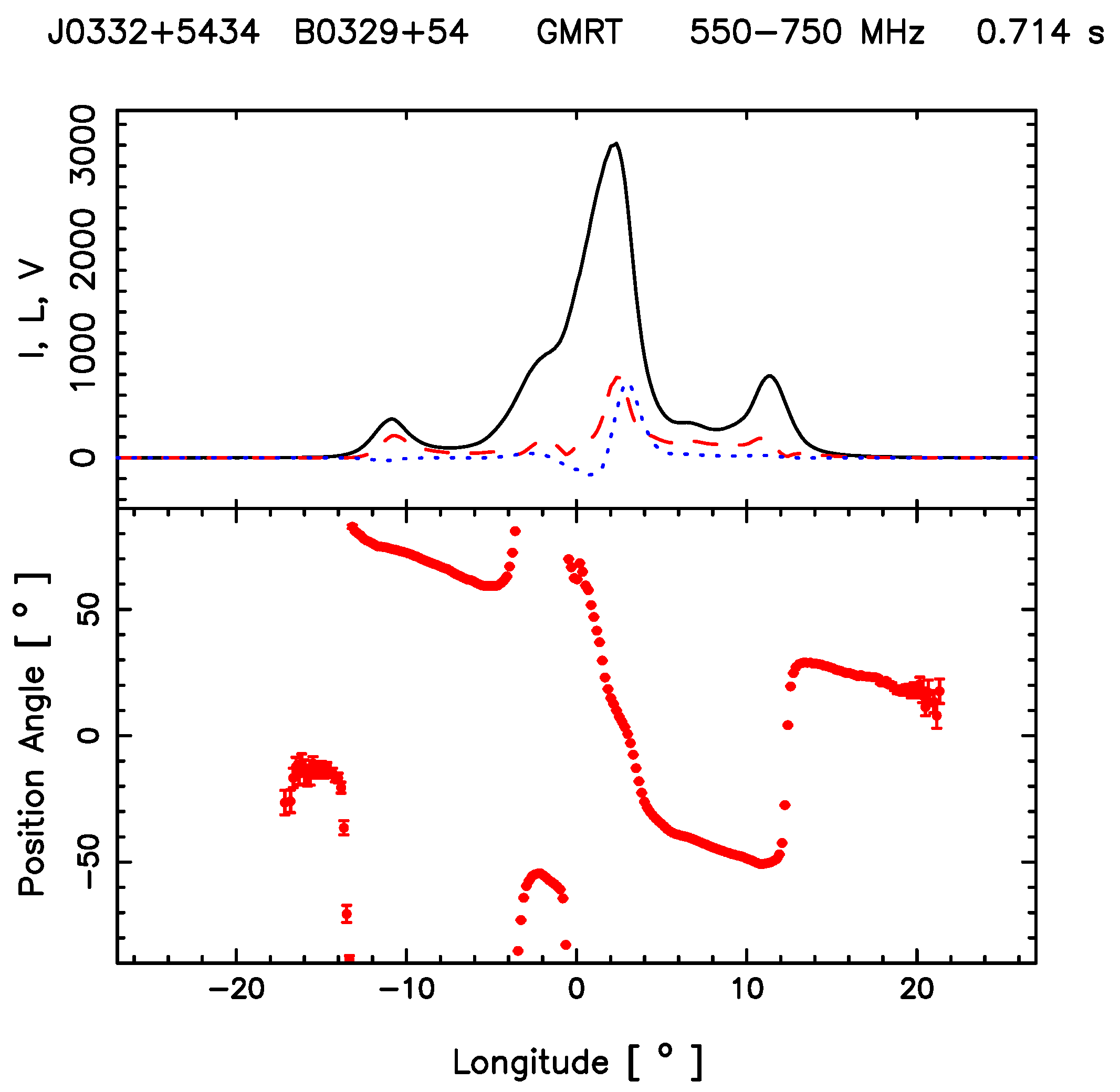

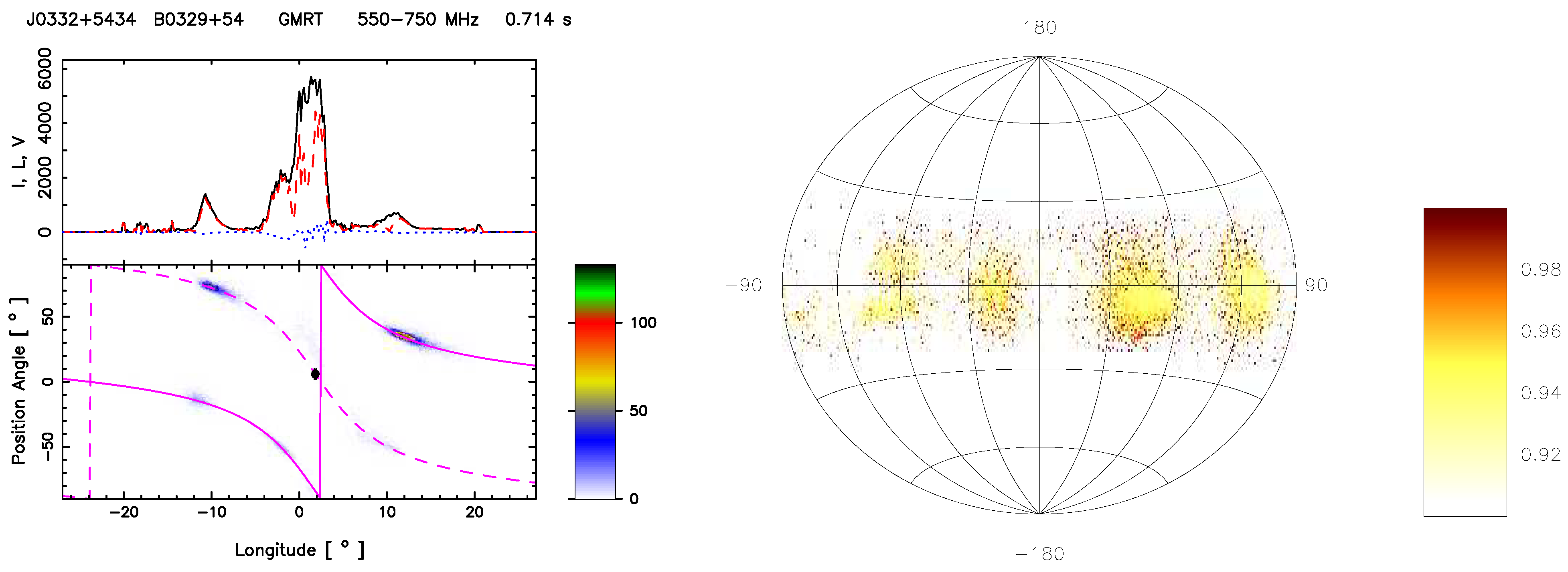
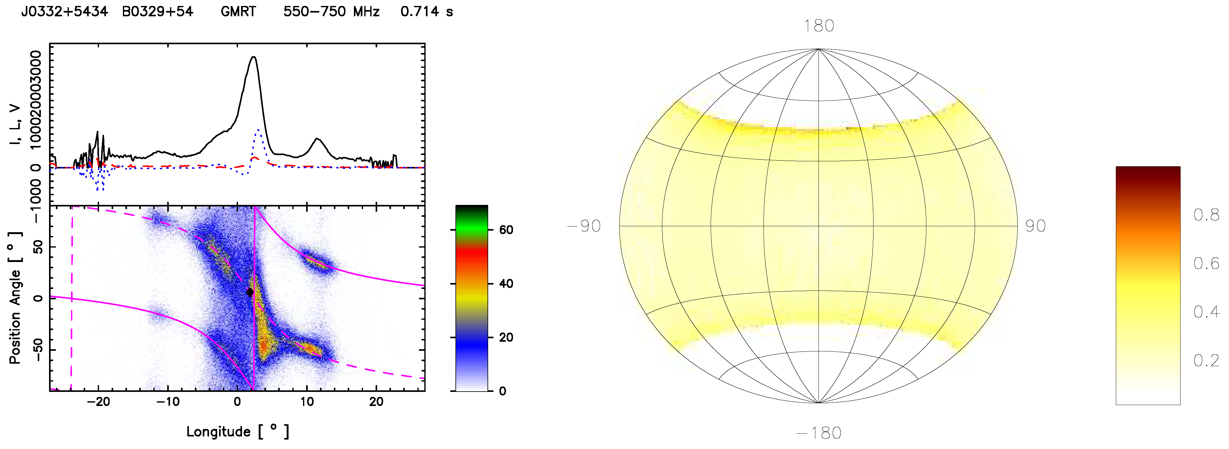
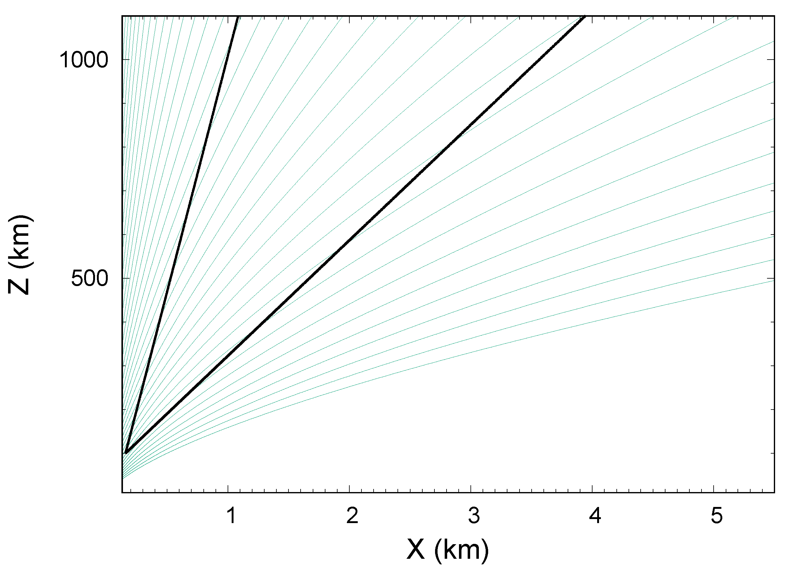

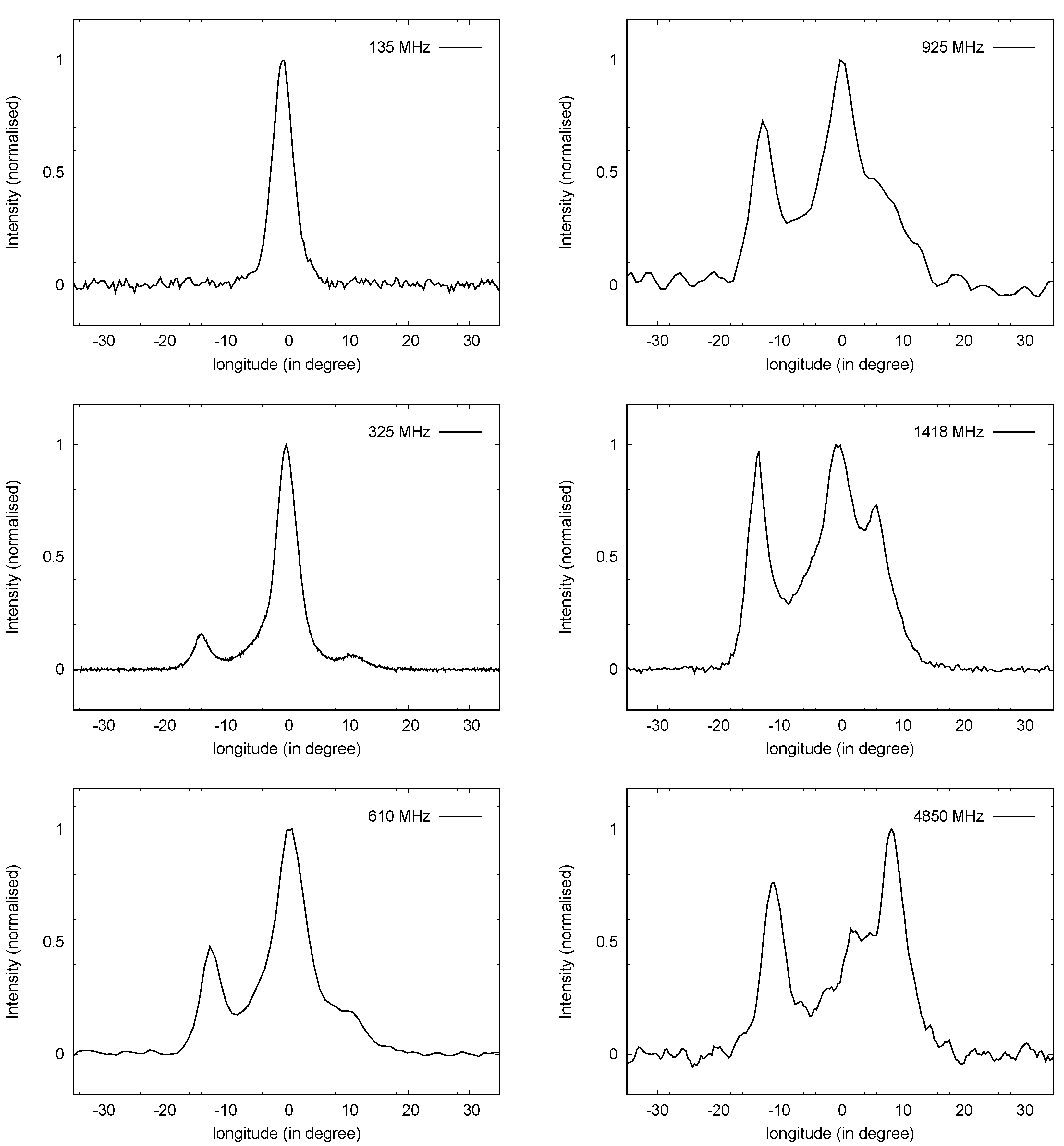


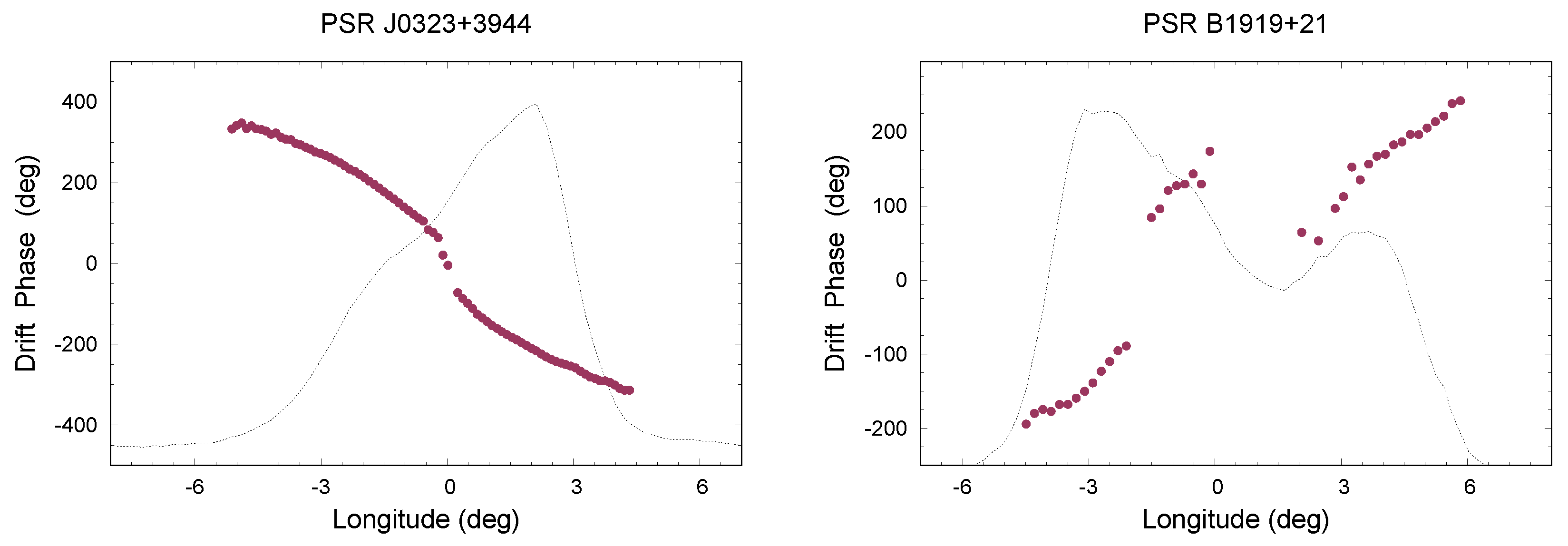
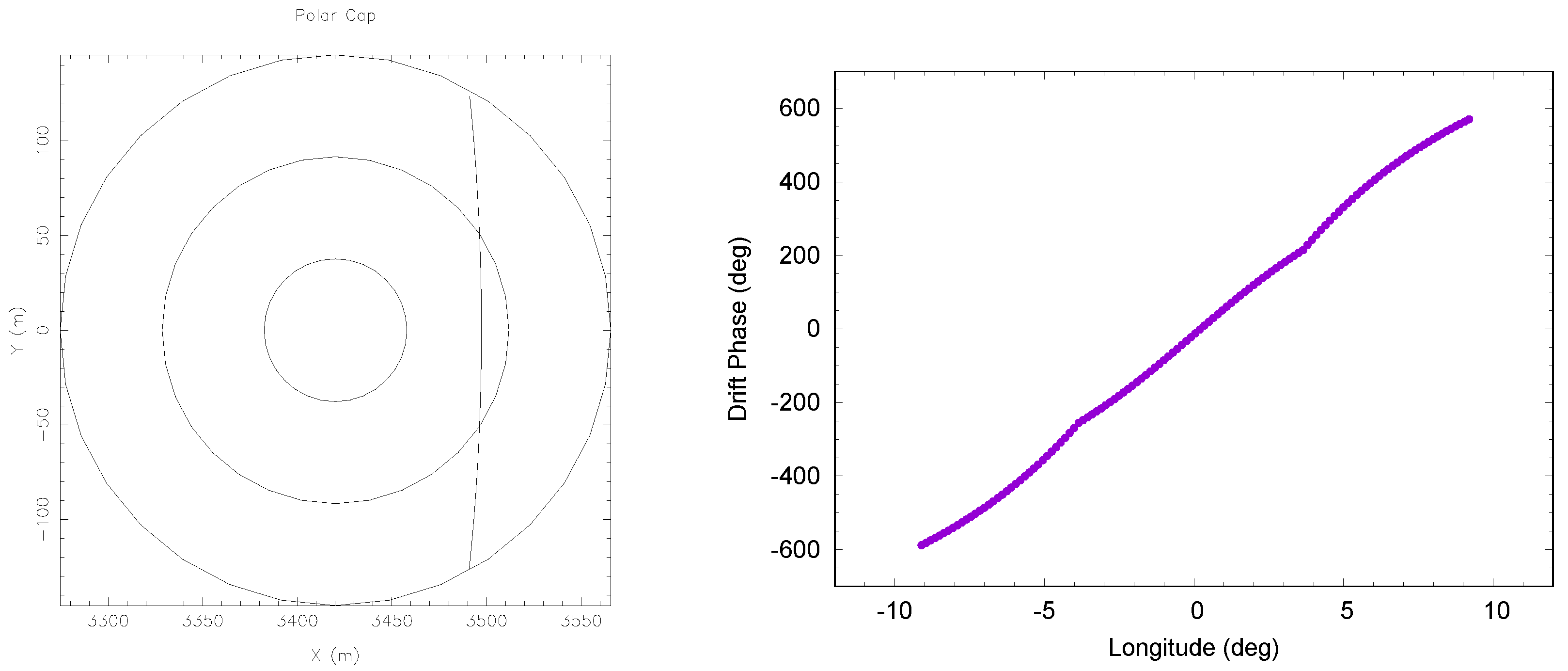

Disclaimer/Publisher’s Note: The statements, opinions and data contained in all publications are solely those of the individual author(s) and contributor(s) and not of MDPI and/or the editor(s). MDPI and/or the editor(s) disclaim responsibility for any injury to people or property resulting from any ideas, methods, instructions or products referred to in the content. |
© 2024 by the authors. Licensee MDPI, Basel, Switzerland. This article is an open access article distributed under the terms and conditions of the Creative Commons Attribution (CC BY) license (https://creativecommons.org/licenses/by/4.0/).